
Excel for Microsoft 365 Excel for Microsoft 365 for Mac Excel for the web Excel 2021 Excel 2021 for Mac Excel 2019 Excel 2019 for Mac Excel 2016 Excel 2016 for Mac Excel 2013 Excel 2010 Excel 2007 Excel for Mac 2011 Excel Starter 2010 More…Less
Description
The ROUND function rounds a number to a specified number of digits. For example, if cell A1 contains 23.7825, and you want to round that value to two decimal places, you can use the following formula:
=ROUND(A1, 2)
The result of this function is 23.78.
Syntax
ROUND(number, num_digits)
The ROUND function syntax has the following arguments:
-
number Required. The number that you want to round.
-
num_digits Required. The number of digits to which you want to round the number argument.
Remarks
-
If num_digits is greater than 0 (zero), then number is rounded to the specified number of decimal places.
-
If num_digits is 0, the number is rounded to the nearest integer.
-
If num_digits is less than 0, the number is rounded to the left of the decimal point.
-
To always round up (away from zero), use the ROUNDUP function.
-
To always round down (toward zero), use the ROUNDDOWN function.
-
To round a number to a specific multiple (for example, to round to the nearest 0.5), use the MROUND function.
Example
Copy the example data in the following table, and paste it in cell A1 of a new Excel worksheet. For formulas to show results, select them, press F2, and then press Enter. If you need to, you can adjust the column widths to see all the data.
|
Formula |
Description |
Result |
|
=ROUND(2.15, 1) |
Rounds 2.15 to one decimal place |
2.2 |
|
=ROUND(2.149, 1) |
Rounds 2.149 to one decimal place |
2.1 |
|
=ROUND(-1.475, 2) |
Rounds -1.475 to two decimal places |
-1.48 |
|
=ROUND(21.5, -1) |
Rounds 21.5 to one decimal place to the left of the decimal point |
20 |
|
=ROUND(626.3,-3) |
Rounds 626.3 to the nearest multiple of 1000 |
1000 |
|
=ROUND(1.98,-1) |
Rounds 1.98 to the nearest multiple of 10 |
0 |
|
=ROUND(-50.55,-2) |
Rounds -50.55 to the nearest multiple of 100 |
-100 |
Need more help?
Want more options?
Explore subscription benefits, browse training courses, learn how to secure your device, and more.
Communities help you ask and answer questions, give feedback, and hear from experts with rich knowledge.
GENERIC FORMULA
=IF(value>=greater_equal_value,ROUND(value,0),value)
ARGUMENTS
value: The value that you want to round if it’s greater than or equal to a specific value.
greater_equal_value: The greater than or equal to number.
GENERIC FORMULA
=IF(value>=greater_equal_value,ROUND(value,0),value)
ARGUMENTS
value: The value that you want to round if it’s greater than or equal to a specific value.
greater_equal_value: The greater than or equal to number.
EXPLANATION
This formula uses the IF function to check if the value that is to be rounded is greater than or equal to a specific number. If the IF function returns a TRUE value, meaning that the number that is being tested is greater than or equal to a specific number, the formula will round the number through the use of the ROUND function. If the number is less than the specific value the formula will return the exact number that is being tested, without rounding it.
Click on either the Hard Coded or Cell Reference button to view the formula that has the greater than or equal to value and the number that is being tested directly entered into the formula or referenced to specific cells.
Содержание
- Round a number
- Change the number of decimal places displayed without changing the number
- On a worksheet
- In a built-in number format
- Round a number up
- Round a number down
- Round a number to the nearest number
- Round a number to a near fraction
- Round a number to a significant digit
- Round a number to a specified multiple
- How to round numbers in Excel: ROUND, ROUNDUP, ROUNDDOWN functions
- Excel rounding by changing the cell format
- Excel functions to round numbers
- Excel ROUND function
- Excel ROUNDUP function
- Excel ROUNDDOWN function
- Excel MROUND function
- Excel FLOOR function
- Excel CEILING function
- Excel INT function
- Excel TRUNC function
- Excel ODD and EVEN functions
- Using rounding formulas in Excel
- How to round decimals in Excel to a certain number of places
- Rounding negative numbers (ROUND, ROUNDDOWN, ROUNDUP)
- How to extract a decimal part of a number
- How to round a decimal to an integer in Excel
- ROUNDUP
- INT or ROUNDDOW
- TRUNC
- ODD or EVEN
- Round to nearest 0.5
- Round to nearest 5 / 10 / 100 / 1000
- Round to nearest 5
- Round to nearest 10
- Round to nearest 100
- Round to nearest 1000
- Rounding time in Excel
- Example 1. How to round time to nearest hour in Excel
- Example 2. Rounding time to nearest 5, 10, 15, etc. minutes
Round a number
Let’s say you want to round a number to the nearest whole number because decimal values are not significant to you. Or, you want to round a number to multiples of 10 to simplify an approximation of amounts. There are several ways to round a number.
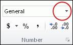
Change the number of decimal places displayed without changing the number
On a worksheet
Select the cells that you want to format.
To display more or fewer digits after the decimal point, on the Home tab, in the Number group, click Increase Decimal  or Decrease Decimal
  .
.
In a built-in number format
On the Home tab, in the Number group, click the arrow next to the list of number formats, and then click More Number Formats.
In the Category list, depending on the data type of your numbers, click Currency, Accounting, Percentage, or Scientific.
In the Decimal places box, enter the number of decimal places that you want to display.
Round a number up
Use the ROUNDUP function. In some cases, you may want to use the EVEN and the ODD functions to round up to the nearest even or odd number.
Round a number down
Use the ROUNDDOWNfunction.
Round a number to the nearest number
Use the ROUND function.
Round a number to a near fraction
Use the ROUND function.
Round a number to a significant digit
Significant digits are digits that contribute to the accuracy of a number.
The examples in this section use the ROUND, ROUNDUP, and ROUNDDOWN functions. They cover rounding methods for positive, negative, whole, and fractional numbers, but the examples shown represent only a very small list of possible scenarios.
The following list contains some general rules to keep in mind when you round numbers to significant digits. You can experiment with the rounding functions and substitute your own numbers and parameters to return the number of significant digits that you want.
When rounding a negative number, that number is first converted to its absolute value (its value without the negative sign). The rounding operation then occurs, and then the negative sign is reapplied. Although this may seem to defy logic, it is the way rounding works. For example, using the ROUNDDOWN function to round -889 to two significant digits results in -880. First, -889 is converted to its absolute value of 889. Next, it is rounded down to two significant digits results (880). Finally, the negative sign is reapplied, for a result of -880.
Using the ROUNDDOWN function on a positive number always rounds a number down, and ROUNDUP always rounds a number up.
The ROUND function rounds a number containing a fraction as follows: If the fractional part is 0.5 or greater, the number is rounded up. If the fractional part is less than 0.5, the number is rounded down.
The ROUND function rounds a whole number up or down by following a similar rule to that for fractional numbers; substituting multiples of 5 for 0.5.
As a general rule, when you round a number that has no fractional part (a whole number), you subtract the length from the number of significant digits to which you want to round. For example, to round 2345678 down to 3 significant digits, you use the ROUNDDOWN function with the parameter -4, as follows: = ROUNDDOWN(2345678,-4). This rounds the number down to 2340000, with the «234» portion as the significant digits.
Round a number to a specified multiple
There may be times when you want to round to a multiple of a number that you specify. For example, suppose your company ships a product in crates of 18 items. You can use the MROUND function to find out how many crates you will need to ship 204 items. In this case, the answer is 12, because 204 divided by 18 is 11.333, and you will need to round up. The 12th crate will contain only 6 items.
There may also be times where you need to round a negative number to a negative multiple or a number that contains decimal places to a multiple that contains decimal places. You can also use the MROUND function in these cases.
Источник
How to round numbers in Excel: ROUND, ROUNDUP, ROUNDDOWN functions
 by Svetlana Cheusheva, updated on February 7, 2023
The tutorial explains the uses of ROUND, ROUNDUP, ROUNDDOWN, FLOOR, CEILING, MROUND and other Excel rounding functions and provides formula examples to round decimal numbers to integers or to a certain number of decimal places, extract a fractional part, round to nearest 5, 10 or 100, and more.
In some situations when you don’t need an exact answer, rounding is a useful skill to use. In plain English, to round a number is to eliminate the least significant digits, making it simpler but keeping close to the original value. In other words, rounding lets you get an approximate number with the desired level of accuracy.
In everyday life, rounding is commonly used to make numbers easier to estimate, communicate or work with. For instance, you can use rounding to make long decimal numbers shorter to report the results of complex calculations or round off currency values.
Many different ways of rounding exist, such as rounding to integer, rounding to a specified increment, rounding to simple fractions, and so on. And Microsoft Excel provides a handful of functions to handle different rounding types. Below, you will find a quick overview of the major round functions and well as formula examples that demonstrate how to use those functions on the real-life data in your worksheets.
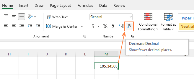
Excel rounding by changing the cell format
If you want to round numbers solely for presentations purposes, then you can just change the number of displayed decimal places without changing the underlying value. The fastest way is to use the Increase Decimal or Decrease Decimal command on the Home tab in the Number group:
Or you can change the cell’s format by performing these steps:
- Select the cell with the number(s) you want to round.
- Open the Format Cells dialog by pressing Ctrl + 1 or right click the cell(s) and choose Format Cells. from the context menu.
- In the Format Cells window, switch to either Number or Currency tab, and type the number of decimal places you want to display in the Decimal places box. A preview of the rounded number will immediately show up under Sample.
- Click the OK button to save the changes and close the Format Cells dialog.
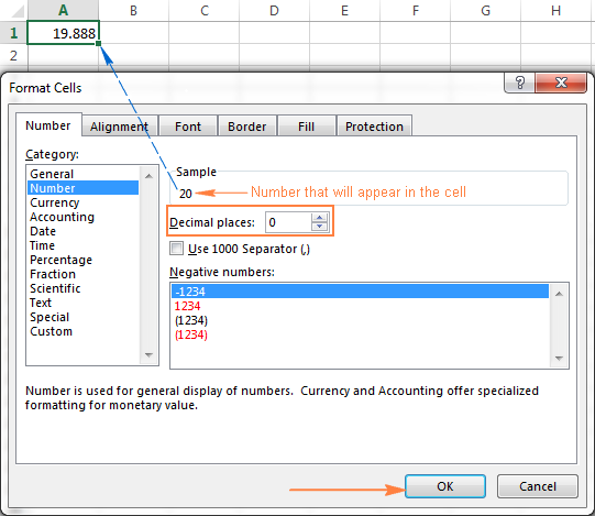
Important note! This method changes the display format without changing the actual value stored in a cell. If you refer to that cell in any formulas, the original non-round value will be used in all calculations.
Excel functions to round numbers
Unlike formatting options that change only the display value, Excel round functions alter the actual value in a cell.
Below you will find a list of functions specially designed for performing different types of rounding in Excel.
- ROUND — round the number to the specified number of digits.
- ROUNDUP — round the number upward to the specified number of digits.
- ROUNDDOWN — round the number downward to the specified number of digits.
- MROUND — rounds the number upward or downward to the specified multiple.
- FLOOR — round the number down to the specified multiple.
- CEILING — round the number up to the specified multiple.
- INT — round the number down to the nearest integer.
- TRUNC — truncate the number to a specified number of decimal places.
- EVEN — round the number up to the nearest even integer.
- ODD — round the number up to the nearest odd integer.
Excel ROUND function
ROUND is the major rounding function in Excel that rounds a numeric value to a specified number of digits.
Syntax: ROUND(number, num_digits)
Number — any real number you want to round. This can be a number, reference to a cell containing the number or a formula-driven value.
Num_digits — the number of digits to round the number to. You can supply a positive or negative value in this argument:
- If num_digits is greater than 0, the number is rounded to the specified number of decimal places.
For example =ROUND(15.55,1) rounds 15.55 to 15.6.
If num_digits is less than 0, all decimal places are removed and the number is rounded to the left of the decimal point (to the nearest ten, hundred, thousand, etc.).
For example =ROUND(15.55,-1) rounds 15.55 to the nearest 10 and returns 20 as the result.
If num_digits equals 0, the number is rounded to the nearest integer (no decimal places).
For example =ROUND(15.55,0) rounds 15.55 to 16.
The Excel ROUND function follows the general math rules for rounding, where the number to the right of the rounding digit determines whether the number is rounded upwards or downwards.
Rounding digit is the last significant digit retained once the number is rounded, and it gets changed depending on whether the digit that follows it is greater or less than 5:
- If the digit to the right of the rounding digit is 0, 1, 2, 3, or 4, the rounding digit is not changed, and the number is said to be rounded down.
- If the rounding digit is followed by 5, 6, 7, 8, or 9, the rounding digit is increased by one, and the number is rounded up.
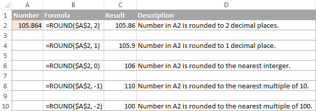
The following screenshot demonstrates a few ROUND formula examples:
Excel ROUNDUP function
The ROUNDUP function rounds the number upward (away from 0) to a specified number of digits.
Syntax: ROUNDUP(number, num_digits)
Number — the number to be rounded up.
Num_digits — the number of digits you want to round the number to. You can supply both positive and negative numbers in this argument, and it works like num_digits of the ROUND function discussed above, except that a number is always rounded upward.
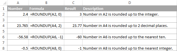
Excel ROUNDDOWN function
The ROUNDDOWN function in Excel does the opposite of what ROUNDUP does, i.e. rounds a number down, toward zero.
Syntax: ROUNDDOWN(number, num_digits)
Number — the number to be rounded down.
Num_digits — the number of digits you want to round the number to. It works like the num_digits argument of the ROUND function, except that a number is always rounded downward.
The following screenshot demonstrates the ROUNDDOWN function in action.
Excel MROUND function
The MROUND function in Excel rounds a given number up or down to the specified multiple.
Syntax: MROUND(number, multiple)
Number — the value you want to round.
Multiple — the multiple to which you want to round the number.
For example, the below formula rounds 7 to the nearest multiple of 2 and returns 8 as the result:
Whether the last remaining digit is rounded up (away from 0) or down (towards 0) depends on the remainder from dividing the number argument by the multiple argument:
- If the remainder is equal to or greater than half the value of the multiple argument, Excel MROUND rounds the last digit up.
- If the remainder is less than half the value of the multiple argument, the last digit is rounded down.
The MROUND function comes in handy, say, for rounding prices to the nearest nickel (5 cents) or a dime (10 cents) to avoid dealing with pennies as change.

And, it is really indispensable when it comes to rounding times to a desired interval. For example, to round time to the nearest 5 or 10 minutes, just supply «0:05» or «0:10» for the multiple, like this:
=MROUND(A2,»0:05″) or =MROUND(A2,»0:10″)

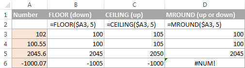
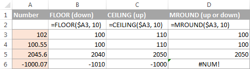
Note. The MROUND function returns the #NUM! error when its arguments have different signs. For example, both of the formulas =MROUND(3, -2) and =MROUND(-5, 2) result in the NUM error.
Excel FLOOR function
The FLOOR function in Excel is used to round a given number down, to the nearest multiple of a specified significance.
Syntax: FLOOR(number, significance)
Number — the number you want to round.
Significance — the multiple to which you wish to round the number.
For example, =FLOOR(2.5, 2) rounds 2.5 down to the nearest multiple of 2, which is 2.
The Excel FLOOR function performs rounding based on the following rules:
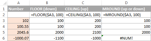
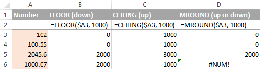
- If the number and significance arguments are positive, the number is rounded down, toward zero, as in rows 2 and 10 in the screenshot below.
- If number is positive and significance is negative, the FLOOR function returns the #NUM error, as in row 4.
- If number is negative and significance is positive, the value is rounded down, away from zero, as in row 6.
- If number and significance are negative, the number is rounded up, toward zero, as in row 8.
- If number is an exact multiple of the significance argument, no rounding takes place.
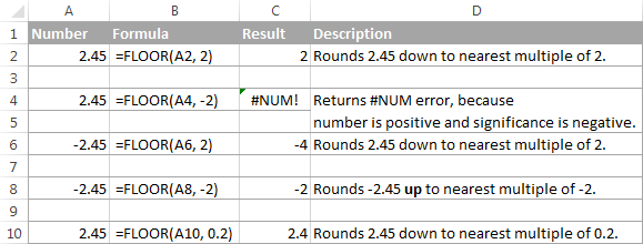
Note. In Excel 2003 & 2007, the number and significance arguments must have the same sign, either positive or negative, otherwise an error is returned. In newer Excel versions, the FLOOR function has been improved, so in Excel 2010, 2013 and 2016 it can handle a negative number and positive significance.
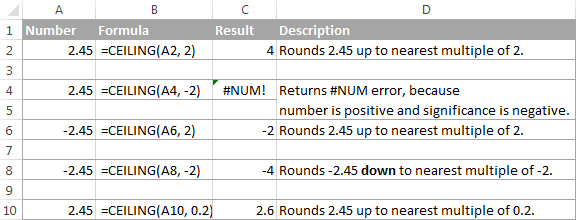
Excel CEILING function
The CEILING function in Excel rounds a given number up, to the nearest multiple of significance. It has the same syntax as the FLOOR function.
Syntax: CEILING(number, significance)
Number — the number you want to round.
Significance — the multiple to which you want to round the number.
For instance, the formula =CEILING(2.5, 2) rounds 2.5 up to the nearest multiple of 2, which is 4.
The Excel CEILING function works based on the rounding rules similar to FLOOR’s, except that it generally rounds up, away from 0.
- If both the number and significance arguments are positive, the number is rounded up, as in rows 2 and 10 in the screenshot below.
- If number is positive and significance is negative, the CEILING function returns the #NUM error, as in row 4.
- If number is negative and significance is positive, the value is rounded up, towards zero, as in row 6.
- If number and significance are negative, the value is rounded down, as in row 8.
Excel INT function
The INT function rounds a number down to the nearest integer.
Of all Excel round functions, INT is probably the easiest one to use, because it requires only one argument.
Number — the number you want to round down to the nearest integer.
Positive numbers are rounded toward 0 while negative numbers are rounded away from 0. For example, =INT(1.5) returns 1 and =INT(-1.5) returns -2.

Excel TRUNC function
The TRUNC function truncates a given numeric value to a specified number of decimal places.
Syntax: TRUNC(number, [num_digits])
- Number — any real number that you want to truncate.
- Num_digits — an optional argument that defines the precision of the truncation, i.e. the number of decimal places to truncate the number to. If omitted, the number is truncated to an integer (zero decimal places).
The Excel TRUNC function adheres to the following rounding rules:
- If num_digits is positive, the number is truncated to the specified number of digits to the right of the decimal point.
- If num_digits is negative, the number is truncated to the specified number of digits to the left of the decimal point.
- If num_digits is 0 or omitted, it rounds the number to an integer. In this case, the TRUNC function works similarly to INT in that both return integers. However, TRUNC simply removes the factional part, while INT rounds a number down to the nearest integer.For example, =TRUNC(-2.4) returns -2, while =INT(-2.4) returns -3 because it’s the lower integer. For more info, please see Rounding to integer example.
The following screenshot demonstrates the TRUNC function in action:

Excel ODD and EVEN functions
These are two more functions provided by Excel for rounding a specified number to an integer.
ODD(number) rounds up to the nearest odd integer.
EVEN(number) rounds up to the nearest even integer.
- In both functions, number is any real number that you want to round.
- If number is non-numeric, the functions return the #VALUE! error.
- If number is negative, it is rounded away from zero.
The ODD and EVEN functions may prove useful when you are processing items that come in pairs.
=ODD(2.4) returns 3
=ODD(-2.4) returns -3
=EVEN(2.4) returns 4
=EVEN(-2.4) returns -4

Using rounding formulas in Excel
As you see, there exist a variety of functions to round off numbers in Excel depending on the particular purpose. The following examples will hopefully give you some clues on how to use Excel rounding formulas based on your criteria.
How to round decimals in Excel to a certain number of places
Depending on the situation, you may want to round decimals up, down or based on math rounding rules:
ROUNDUP function — always rounds the decimal upward.
ROUNDDOWN function — always rounds the decimal downward.
ROUND — rounds up if the rounding digit is followed by the digit equal to or greater than 5, otherwise rounds down.
As an example, lets round the decimal numbers in column A to 2 decimal places. In the first argument (number), you enter a reference to the cell containing the number, and in the second argument (num_digits) you specify the number of decimal places you want to keep.
=ROUNDUP(A2, 2) — rounds the number in A2 upward, to two decimal places.
=ROUNDDOWN(A2, 2) — rounds the number in A2 downward, to two decimal places.
=ROUND(A2, 2) — rounds the number in A2 to 2 decimal places, upward or downward, depending on whether the 3 rd decimal digit is greater or less than 5.

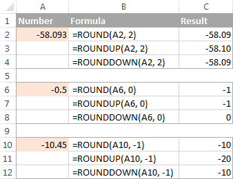
Rounding negative numbers (ROUND, ROUNDDOWN, ROUNDUP)
When it comes to rounding a negative number, the results returned by the Excel round functions, may seem to flout logic 🙂
When the ROUNDUP function applies to negative numbers, they are said to be rounded up, even though they actually decrease in value. For example, the result of =ROUNDUP(-0.5, 0) is -1, as in row 7 in the screenshot below.
The ROUNDDOWN function is known to round numbers downward, though negative numbers may increase in value. For example, the formula =ROUNDDOWN(-0.5, 0) returns 0, as in row 8 in the screenshot below.
In fact, the rounding logic with regard to negative numbers is very simple. Whenever you use the ROUND, ROUNDDOWN or ROUNDUP function in Excel on a negative number, that number is first converted to its absolute value (without the minus sign), then the rounding operation occurs, and then the negative sign is re-applied to the result.
If you want to extract a fractional part of a decimal number, you can use the TRUNC function to truncate the decimal places and then subtract that integer from the original decimal number.
As demonstrated in the screenshot below, the formula in column B works perfectly both for positive and negative numbers. However, if you’d rather get an absolute value (decimal part without the minus sign), then wrap the formula in the ABS function:

How to round a decimal to an integer in Excel
As is the case with rounding to a certain number of decimal places, there is a handful of functions for rounding a fractional number to an integer.
ROUNDUP
To round up to nearest integer, use an Excel ROUNDUP formula with num_digits set to 0. For example =ROUNDUP(5.5, 0) rounds decimal 5.5 to 6.
INT or ROUNDDOW
To round down to nearest whole number, use either INT or ROUNDDOW with num_digits set to 0. For example both of the following formulas round 5.5 to 5:
For negative decimals, however, the INT and ROUNDDOWN functions yield different results — INT rounds negative decimals away from 0, while ROUNDDOWN toward 0:
=ROUNDOWN(-5.5, 0) returns -5.
=INT(-5.5) returns -6.
TRUNC
To remove the factional part without changing the integer part, use the TRUNC formula with the second argument (num_digits) omitted or set to 0. For example, =TRUNC(5.5) truncates the decimal part (.5) and returns the integer part (5).
ODD or EVEN
To round a decimal up to the nearest odd integer, use the ODD function:
=ODD(5.5) returns 7.
To round a decimal up to the nearest even integer, use the EVEN function:
=EVEN(5.5) returns 6.

Round to nearest 0.5
Microsoft Excel provides 3 functions that let you round numbers to nearest half, more precisely to the nearest multiple of 0.5. Which one to use depends on your rounding criteria.
- To round a number down to nearest 0.5, use the FLOOR function, for example =FLOOR(A2, 0.5) .
- To round a number up to nearest 0.5, use the CEILING function, for example =CEILING(A2, 0.5) .
- To round a number up or down to nearest 0.5, use the MROUND function, e.g. =MROUND(A2, 0.5) . Whether MROUND rounds the number up or down depends on the remainder from dividing the number by multiple. If the remainder is equal to or greater than half the value of multiple, the number is rounded upward, otherwise downward.
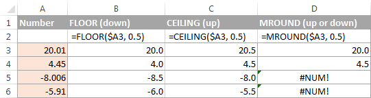
As you see, the MROUND function can be used for rounding positive values only, when applied to negative numbers, it returns the #NUM error.
Round to nearest 5 / 10 / 100 / 1000
Rounding to nearest five, ten, hundred or thousand is done in the same manner as rounding to 0.5 discussed in the previous example.
Round to nearest 5
Supposing that the number you want to round to closest 5 resides in cell A2, you can use on of the following formulas:
- To round a number down to nearest 5:
=FLOOR(A2, 5) - To round a number up to nearest 5:
=CEILING(A2, 5) - To round a number up or down to nearest 5:
=MROUND(A2, 5)
Round to nearest 10
To round your numbers to nearest ten, supply 10 in the second argument of the rounding functions:
- To round a number down to nearest 10:
=FLOOR(A2, 10) - To round a number up to nearest 10:
=CEILING(A2, 10) - To round a number up or down to nearest 10:
=MROUND(A2, 10)
Round to nearest 100
Rounding to a hundred is done in the same way, except that you enter 100 in the second argument:
- To round a number down to nearest 100:
=FLOOR(A2, 100) - To round a number up to nearest 100:
=CEILING(A2, 100) - To round a number up or down to nearest 100
=MROUND(A2, 100)
Round to nearest 1000
To round a value in cell A2 to the nearest thousand, use of the following formulas:
- To round a number down to nearest 1000:
=FLOOR(A2, 1000) - To round a number up to nearest 1000:
=CEILING(A2, 1000) - To round a number up or down to nearest 1000
=MROUND(A2, 1000)
The same techniques can be used for rounding numbers to other multiples. For example, you can round the prices to the nearest nickel (multiple of 0.05), lengths to the nearest inch (multiple of 1/12), or minutes to the nearest second (multiple of 1/60). Speaking of time, and do you know how to convert it to nearest hour or closest 5 or 10 minutes? If you don’t, you will find the answers in the next section 🙂
Rounding time in Excel
There may be many situations when you need to round time values. And again, you can use different rounding functions depending on your purpose.
Example 1. How to round time to nearest hour in Excel
With times located in column A, you can use one of the following functions to round time to nearest hour:
- To round time to closest hour (up or down) — MROUND or ROUND.
=ROUND(A1*24,0)/24
To round up time to nearest hour — ROUNDUP or CEILING.
=ROUNDUP(A1*24,0)/24
To round down time to nearest hour — ROUNDDOWN or FLOOR.
In the ROUND, ROUNDUP and ROUNDDOWN formulas, you multiply the time value by 24 (number of hours in a day) to convert a serial number representing the time to hours. Then you use one of the rounding functions to round the decimal value to an integer, and then divide it by 24 to change the returned value back to the time format.

If your timestamps include date values, then use the INT or TRUNC function to extract dates (in the internal Excel system, dates and times are stored as serial numbers, the integer part representing a date and fractional part representing time). And then, use the formulas described above but subtract the date value. For example:
The following screenshot demonstrates other formulas:

Note. For the results to display correctly, remember to apply the Time format to your cells.
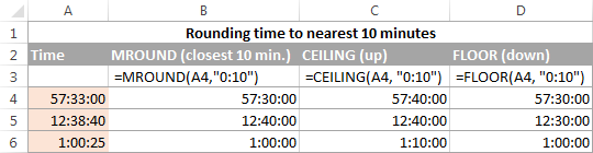
Example 2. Rounding time to nearest 5, 10, 15, etc. minutes
In case you want to round times in your Excel sheet to five or ten minutes, or to the closest quarter-hour, you can use the same rounding techniques as demonstrated above, but replace «1 hour» with the desired number of minutes in the formulas.
For example, to round the time in A1 to the closest 10 minutes, use one of the following functions:
- To round time to closest 10 minutes (up or down): =MROUND(A1,»0:10″)
=MROUND(A1, TIME(0,10,0))
To round up time to nearest 10 min: =CEILING(A1, «0:10»)
=CEILING(A1, TIME(0,10,0))
To round down time to nearest 10 min: =FLOOR(A1, «0:10»)
If you know (or can calculate) what portion of a day is constituted by a certain number of minutes, then you won’t have problems using the ROUND, ROUNDUP and ROUNDOWN functions as well.
For example, knowing that 15 minutes, is 1/96th of a day, you can use one of the following formulas to round the time in A1 to the nearest quarter-hour.
- To round time to closest 15 minutes (up or down): =ROUND(A1*96,0)/96
- To round up time to nearest 15 min: =ROUNDUP(A1*96,0)/96
- To round down time to nearest 15 min: =ROUNDDOWN(A1*96,0)/96
This is how you perform rounding in Excel. Hopefully, now you know how, among all those round functions, chose the one best suited for your needs.
Источник
Purpose
Round a number to a given number of digits
Usage notes
The ROUND function rounds a number to a given number of places. ROUND rounds up when the last significant digit is 5 or greater, and rounds down when the last significant digit is less than 5.
ROUND takes two arguments, number and num_digits. Number is the number to be rounded, and num_digits is the place at which number should be rounded. When num_digits is greater than zero, the ROUND function rounds on the right side of the decimal point. When num_digits is less or equal to zero, the ROUND function rounds on the left side of the decimal point. Use zero (0) for num_digits to round to the nearest integer. This behavior is summarized in the table below:
| Digits | Behavior |
|---|---|
| >0 | Round to nearest .1, .01, .001, etc. |
| <0 | Round to nearest 10, 100, 1000, etc. |
| =0 | Round to nearest 1 |
Round to right
To round values to the right of the decimal point, use a positive number for digits:
=ROUND(A1,1) // Round to 1 decimal place
=ROUND(A1,2) // Round to 2 decimal places
=ROUND(A1,3) // Round to 3 decimal places
=ROUND(A1,4) // Round to 4 decimal places
Round to left
To round down values to the left of the decimal point, use zero or a negative number for digits:
=ROUND(A1,0) // Round to nearest whole number
=ROUND(A1,-1) // Round to nearest 10
=ROUND(A1,-2) // Round to nearest 100
=ROUND(A1,-3) // Round to nearest 1000
=ROUND(A1,-4) // Round to nearest 10000
Nesting inside ROUND
Other operations and functions can be nested inside the ROUND function. For example, to round down the result of A1 divided by B1, you can ROUND in a formula like this:
=ROUND(A1/B1,0) // round result to nearest integer
Any formula that returns a numeric result can be nested inside the ROUND function.
Other rounding functions
Excel provides a number of rounding functions, each with a different behavior:
- To round with standard rules, use the ROUND function.
- To round to the nearest multiple, use the MROUND function.
- To round down to the nearest specified place, use the ROUNDDOWN function.
- To round down to the nearest specified multiple, use the FLOOR function.
- To round up to the nearest specified place, use the ROUNDUP function.
- To round up to the nearest specified multiple, use the CEILING function.
- To round down and return an integer only, use the INT function.
- To truncate decimal places, use the TRUNC function.
Notes
- The ROUND function rounds to a specified level of precision, determined by num_digits.
- If number is already rounded to the given number of places, no rounding occurs.
- If number is not numeric, ROUND returns a #VALUE! error.
|
Jeny Пользователь Сообщений: 4 |
=IF((ROUND(A2/$C$2;2))=OR(0,56;1,56;1,06;2,06);»-4″) |
|
Daulet Пользователь Сообщений: 626 |
с чего Вы взяли что (ОКРУГЛ(A2/$C$2;2))=ИЛИ(0,56;1,56;1,06;2,06) будет равно =ЕСЛИ((ОКРУГЛ(A2/$C$2;2))={0,56;1,56;1,06;2,06};»-4″) |
|
А что Вы хотите получить, если не находит округл()? Зы. И это формула массива,. |
|
|
Daulet Пользователь Сообщений: 626 |
ошибся в этом =ЕСЛИ((ОКРУГЛ(A2/$C$2;2))={0,56;1,56;1,06;2,06};»-4″) |
|
Вообще синтаксис ИЛИ() как-то так: зы и если Вам нужно число, то -4 лучше без кавычек. |
|
|
VLad777 Пользователь Сообщений: 5018 |
вариант переделки вашей формулы не вникая что да зачем |
|
Daulet Пользователь Сообщений: 626 |
=ЕСЛИ(ПОИСКПОЗ(ОКРУГЛ(A2/$C$2;2);{0,56;1,56;1,06;2,06};0);»-4″;»») |
|
vikttur Пользователь Сообщений: 47199 |
И я к гадателям |

|
А вот это уже формула массива. |
|
|
vikttur Пользователь Сообщений: 47199 |
Массива. Констант. Поэтому ввода трехпальцевого не просит. По скорости работы — не знаю. |
|
Jeny Пользователь Сообщений: 4 |
=ЕСЛИ(ЕЧИСЛО(ПОИСКПОЗ(ОКРУГЛ(A2/$C$2;2);{0,56;1,56;1,06;2,06};0));»-4″) |
|
Владимир Пользователь Сообщений: 8196 |
#12 26.06.2012 18:34:32 А зачем Вы создаёте данный массив {0,56;1,56;1,06;2,06} ? «..Сладку ягоду рвали вместе, горьку ягоду я одна.» |
I’m trying to combine an IF function with an round function to try to round a certain value.
In this case the value is in cell H2. E2=decimal places. So if E2=9 there are 9 decimal places. I try to use this formula but it doesn’t work(just based on E2=0 and E2=1).
=IF( E2= 0,ROUND( $H2, 2),IF( E2=1 ,ROUND( $H2, 1))
I get an error, something is wrong in the syntax can someone help me with it?
![]()
asked Sep 26, 2013 at 8:10
![]()
I don’t know whether it is a language setting, but I needed to replace all ‘,’ by ‘;’. Further you missed a closing bracked.
=IF(E2=0;ROUND($H2;2);IF(E2=1;ROUND($H2;1)))
Besides this, I think that
=IFERROR(ROUND($H$2;E2); 0)
would be a better solution to use. Now you don’t need the IF functions.
answered Sep 26, 2013 at 8:15
![]()
RFerwerdaRFerwerda
1,2672 gold badges10 silver badges24 bronze badges
1