
In September, 2018 we announced that Dynamic Array support would be coming to Excel. This allows formulas to spill across multiple cells if the formula returns multi-cell ranges or arrays. This new dynamic array behavior can also affect earlier functions that have the ability to return a multi-cell range or array.
Below is a list of functions that could return multi-cell ranges or arrays in what we refer to as pre-dynamic array Excel. If these functions were used in workbooks predating dynamic arrays, and returned a multi-cell range or array to the grid (or a function that did not expect them), then silent implicit intersection would have occurred. Dynamic array Excel indicates where implicit intersection could occur using the @ operator, and as a result, these functions may be prepended with an @ if they were originally authored in a pre-dynamic array version of Excel. Additionally, if authored on dynamic array Excel, these functions may appear as legacy array formulas in pre-dynamic array Excel unless prepended with @.
-
CELL
-
COLUMN
-
FILTERXML
-
FORMULATEXT
-
FREQUENCY
-
GROWTH
-
HYPERLINK
-
INDEX
-
INDIRECT
-
ISFORMULA
-
LINEST
-
LOGEST
-
MINVERSE
-
MMULT
-
MODE.MULT
-
MUNIT
-
OFFSET
-
ROW
-
TRANSPOSE
-
TREND
-
All User Defined Functions
Need more help?
You can always ask an expert in the Excel Tech Community or get support in the Answers community.
Need more help?
Want more options?
Explore subscription benefits, browse training courses, learn how to secure your device, and more.
Communities help you ask and answer questions, give feedback, and hear from experts with rich knowledge.
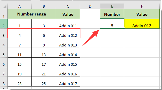
As the left screenshot shown, if a given number 5 is in a certain number range, how to return the value in the adjacent cell. The formula method in this article can help you achieve it.
Return a value if a given value exists in a certain range by using a formula
Return a value if a given value exists in a certain range by using a formula
Please apply the following formula to return a value if a given value exists in a certain range in Excel.
1. Select a blank cell, enter formula =VLOOKUP(E2,A2:C8,3, TRUE) into the Formula Bar and then press the Enter key. See screenshot:
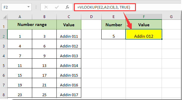
You can see the given number 5 is in the number range 4-6, then the corresponding value Addin 012 in the adjacent cell is populated into the selected cell immediately as above screenshot showed.
Note: In the formula, E2 is the cell contains the given number, A2:C8 contains the number range and the value you will return based on the given number, and number 3 means that the value you will return locates in the third column of range A2:C8. Please change them based on your need.
Related Articles:
- How to vlookup value and return true or false / yes or no in Excel?
- How to vlookup return value in adjacent or next cell in Excel?
- How to return value in another cell if a cell contains certain text in Excel?
The Best Office Productivity Tools
Kutools for Excel Solves Most of Your Problems, and Increases Your Productivity by 80%
- Reuse: Quickly insert complex formulas, charts and anything that you have used before; Encrypt Cells with password; Create Mailing List and send emails…
- Super Formula Bar (easily edit multiple lines of text and formula); Reading Layout (easily read and edit large numbers of cells); Paste to Filtered Range…
- Merge Cells/Rows/Columns without losing Data; Split Cells Content; Combine Duplicate Rows/Columns… Prevent Duplicate Cells; Compare Ranges…
- Select Duplicate or Unique Rows; Select Blank Rows (all cells are empty); Super Find and Fuzzy Find in Many Workbooks; Random Select…
- Exact Copy Multiple Cells without changing formula reference; Auto Create References to Multiple Sheets; Insert Bullets, Check Boxes and more…
- Extract Text, Add Text, Remove by Position, Remove Space; Create and Print Paging Subtotals; Convert Between Cells Content and Comments…
- Super Filter (save and apply filter schemes to other sheets); Advanced Sort by month/week/day, frequency and more; Special Filter by bold, italic…
- Combine Workbooks and WorkSheets; Merge Tables based on key columns; Split Data into Multiple Sheets; Batch Convert xls, xlsx and PDF…
- More than 300 powerful features. Supports Office / Excel 2007-2021 and 365. Supports all languages. Easy deploying in your enterprise or organization. Full features 30-day free trial. 60-day money back guarantee.
")
Office Tab Brings Tabbed interface to Office, and Make Your Work Much Easier
- Enable tabbed editing and reading in Word, Excel, PowerPoint, Publisher, Access, Visio and Project.
- Open and create multiple documents in new tabs of the same window, rather than in new windows.
- Increases your productivity by 50%, and reduces hundreds of mouse clicks for you every day!
")
Comments (14)
No ratings yet. Be the first to rate!
Is there a function that will create a range (from a range) if they match values? Essentially, I’m looking for something like COUNTIF, that will return the cells that actually match my IF.
Ideally, something like RANGEIF(<NORMAL_RANGE_HERE>, ">"&C12), which will return all cells in <NORMAL_RANGE_HERE> that are greater than C12.
![]()
asked Mar 11, 2011 at 16:48
![]()
Glen SolsberryGlen Solsberry
3731 gold badge8 silver badges20 bronze badges
2
The solution here is to use IF, but use it as an array function. For example, if you have this table (sorry for the formatting):
    A   B   C   D
   ______________
1 | 1   3   2   5
2 | 8   1   3   2
3 | 5   4   3   9
Now say you only wanted values that were greater than three in an identical table.
- Select an empty block of cells matching the size of your original table.
- Now type in the formula (remember to make sure you have your whole new cell block selected, very important): =IF(A1:D3>3,A1:D3,»»).
- Now don’t just hit Enter… In order to enter this as an array function you need to hit Ctrl-Shift-Enter.
- Now that one formula is applied to the entire cell block as an ‘array formula’ and it will evaluate the range you put into the IF formula cell by cell depending on the cell’s location in the array. You can tell it was applied as an array formula by clicking on one of the cells. In the formula editor you should see the formula enclosed in curly braces like this: {=IF(A1:D3>3A1:D3,»»)}
You should end up with (assuming your empty block was F1:I3):
    F   G   H   I
   ______________
1 |             5
2 | 8
3 | 5   4       9
Hopefully this is enough to get you going. Do a Google search for «excel array formula» for more info. Hope this helps!
answered Mar 28, 2011 at 20:05
![]()
1