
The IF function allows you to make a logical comparison between a value and what you expect by testing for a condition and returning a result if that condition is True or False.
-
=IF(Something is True, then do something, otherwise do something else)
But what if you need to test multiple conditions, where let’s say all conditions need to be True or False (AND), or only one condition needs to be True or False (OR), or if you want to check if a condition does NOT meet your criteria? All 3 functions can be used on their own, but it’s much more common to see them paired with IF functions.
Use the IF function along with AND, OR and NOT to perform multiple evaluations if conditions are True or False.
Syntax
-
IF(AND()) — IF(AND(logical1, [logical2], …), value_if_true, [value_if_false]))
-
IF(OR()) — IF(OR(logical1, [logical2], …), value_if_true, [value_if_false]))
-
IF(NOT()) — IF(NOT(logical1), value_if_true, [value_if_false]))
|
Argument name |
Description |
|
|
logical_test (required) |
The condition you want to test. |
|
|
value_if_true (required) |
The value that you want returned if the result of logical_test is TRUE. |
|
|
value_if_false (optional) |
The value that you want returned if the result of logical_test is FALSE. |
|
Here are overviews of how to structure AND, OR and NOT functions individually. When you combine each one of them with an IF statement, they read like this:
-
AND – =IF(AND(Something is True, Something else is True), Value if True, Value if False)
-
OR – =IF(OR(Something is True, Something else is True), Value if True, Value if False)
-
NOT – =IF(NOT(Something is True), Value if True, Value if False)
Examples
Following are examples of some common nested IF(AND()), IF(OR()) and IF(NOT()) statements. The AND and OR functions can support up to 255 individual conditions, but it’s not good practice to use more than a few because complex, nested formulas can get very difficult to build, test and maintain. The NOT function only takes one condition.

Here are the formulas spelled out according to their logic:
|
Formula |
Description |
|---|---|
|
=IF(AND(A2>0,B2<100),TRUE, FALSE) |
IF A2 (25) is greater than 0, AND B2 (75) is less than 100, then return TRUE, otherwise return FALSE. In this case both conditions are true, so TRUE is returned. |
|
=IF(AND(A3=»Red»,B3=»Green»),TRUE,FALSE) |
If A3 (“Blue”) = “Red”, AND B3 (“Green”) equals “Green” then return TRUE, otherwise return FALSE. In this case only the first condition is true, so FALSE is returned. |
|
=IF(OR(A4>0,B4<50),TRUE, FALSE) |
IF A4 (25) is greater than 0, OR B4 (75) is less than 50, then return TRUE, otherwise return FALSE. In this case, only the first condition is TRUE, but since OR only requires one argument to be true the formula returns TRUE. |
|
=IF(OR(A5=»Red»,B5=»Green»),TRUE,FALSE) |
IF A5 (“Blue”) equals “Red”, OR B5 (“Green”) equals “Green” then return TRUE, otherwise return FALSE. In this case, the second argument is True, so the formula returns TRUE. |
|
=IF(NOT(A6>50),TRUE,FALSE) |
IF A6 (25) is NOT greater than 50, then return TRUE, otherwise return FALSE. In this case 25 is not greater than 50, so the formula returns TRUE. |
|
=IF(NOT(A7=»Red»),TRUE,FALSE) |
IF A7 (“Blue”) is NOT equal to “Red”, then return TRUE, otherwise return FALSE. |
Note that all of the examples have a closing parenthesis after their respective conditions are entered. The remaining True/False arguments are then left as part of the outer IF statement. You can also substitute Text or Numeric values for the TRUE/FALSE values to be returned in the examples.
Here are some examples of using AND, OR and NOT to evaluate dates.

Here are the formulas spelled out according to their logic:
|
Formula |
Description |
|---|---|
|
=IF(A2>B2,TRUE,FALSE) |
IF A2 is greater than B2, return TRUE, otherwise return FALSE. 03/12/14 is greater than 01/01/14, so the formula returns TRUE. |
|
=IF(AND(A3>B2,A3<C2),TRUE,FALSE) |
IF A3 is greater than B2 AND A3 is less than C2, return TRUE, otherwise return FALSE. In this case both arguments are true, so the formula returns TRUE. |
|
=IF(OR(A4>B2,A4<B2+60),TRUE,FALSE) |
IF A4 is greater than B2 OR A4 is less than B2 + 60, return TRUE, otherwise return FALSE. In this case the first argument is true, but the second is false. Since OR only needs one of the arguments to be true, the formula returns TRUE. If you use the Evaluate Formula Wizard from the Formula tab you’ll see how Excel evaluates the formula. |
|
=IF(NOT(A5>B2),TRUE,FALSE) |
IF A5 is not greater than B2, then return TRUE, otherwise return FALSE. In this case, A5 is greater than B2, so the formula returns FALSE. |

Using AND, OR and NOT with Conditional Formatting
You can also use AND, OR and NOT to set Conditional Formatting criteria with the formula option. When you do this you can omit the IF function and use AND, OR and NOT on their own.
From the Home tab, click Conditional Formatting > New Rule. Next, select the “Use a formula to determine which cells to format” option, enter your formula and apply the format of your choice.

Using the earlier Dates example, here is what the formulas would be.

|
Formula |
Description |
|---|---|
|
=A2>B2 |
If A2 is greater than B2, format the cell, otherwise do nothing. |
|
=AND(A3>B2,A3<C2) |
If A3 is greater than B2 AND A3 is less than C2, format the cell, otherwise do nothing. |
|
=OR(A4>B2,A4<B2+60) |
If A4 is greater than B2 OR A4 is less than B2 plus 60 (days), then format the cell, otherwise do nothing. |
|
=NOT(A5>B2) |
If A5 is NOT greater than B2, format the cell, otherwise do nothing. In this case A5 is greater than B2, so the result will return FALSE. If you were to change the formula to =NOT(B2>A5) it would return TRUE and the cell would be formatted. |
Note: A common error is to enter your formula into Conditional Formatting without the equals sign (=). If you do this you’ll see that the Conditional Formatting dialog will add the equals sign and quotes to the formula — =»OR(A4>B2,A4<B2+60)», so you’ll need to remove the quotes before the formula will respond properly.
Need more help?

See also
You can always ask an expert in the Excel Tech Community or get support in the Answers community.
Learn how to use nested functions in a formula
IF function
AND function
OR function
NOT function
Overview of formulas in Excel
How to avoid broken formulas
Detect errors in formulas
Keyboard shortcuts in Excel
Logical functions (reference)
Excel functions (alphabetical)
Excel functions (by category)
Содержание
- Using IF with AND, OR and NOT functions
- Examples
- Using AND, OR and NOT with Conditional Formatting
- Need more help?
- See also
- Use AND and OR to test a combination of conditions
- Use AND and OR with IF
- Sample data
- Excel IF OR function with formula examples
- IF OR statement in Excel
- Excel IF OR formula examples
- Formula 1. IF with multiple OR conditions
- Formula 2. If a cell is this OR that, then calculate
- Formula 3. Case-sensitive IF OR formula
- Formula 4. Nested IF OR statements in Excel
- Formula 5. IF AND OR statement
- You may also be interested in
Using IF with AND, OR and NOT functions
The IF function allows you to make a logical comparison between a value and what you expect by testing for a condition and returning a result if that condition is True or False.
=IF(Something is True, then do something, otherwise do something else)
But what if you need to test multiple conditions, where let’s say all conditions need to be True or False ( AND), or only one condition needs to be True or False ( OR), or if you want to check if a condition does NOT meet your criteria? All 3 functions can be used on their own, but it’s much more common to see them paired with IF functions.
Use the IF function along with AND, OR and NOT to perform multiple evaluations if conditions are True or False.
IF(AND()) — IF(AND(logical1, [logical2], . ), value_if_true, [value_if_false]))
IF(OR()) — IF(OR(logical1, [logical2], . ), value_if_true, [value_if_false]))
IF(NOT()) — IF(NOT(logical1), value_if_true, [value_if_false]))
The condition you want to test.
The value that you want returned if the result of logical_test is TRUE.
The value that you want returned if the result of logical_test is FALSE.
Here are overviews of how to structure AND, OR and NOT functions individually. When you combine each one of them with an IF statement, they read like this:
AND – =IF(AND(Something is True, Something else is True), Value if True, Value if False)
OR – =IF(OR(Something is True, Something else is True), Value if True, Value if False)
NOT – =IF(NOT(Something is True), Value if True, Value if False)
Examples
Following are examples of some common nested IF(AND()), IF(OR()) and IF(NOT()) statements. The AND and OR functions can support up to 255 individual conditions, but it’s not good practice to use more than a few because complex, nested formulas can get very difficult to build, test and maintain. The NOT function only takes one condition.
Here are the formulas spelled out according to their logic:
=IF(AND(A2>0,B2 0,B4 50),TRUE,FALSE)
IF A6 (25) is NOT greater than 50, then return TRUE, otherwise return FALSE. In this case 25 is not greater than 50, so the formula returns TRUE.
IF A7 (“Blue”) is NOT equal to “Red”, then return TRUE, otherwise return FALSE.
Note that all of the examples have a closing parenthesis after their respective conditions are entered. The remaining True/False arguments are then left as part of the outer IF statement. You can also substitute Text or Numeric values for the TRUE/FALSE values to be returned in the examples.
Here are some examples of using AND, OR and NOT to evaluate dates.
Here are the formulas spelled out according to their logic:
IF A2 is greater than B2, return TRUE, otherwise return FALSE. 03/12/14 is greater than 01/01/14, so the formula returns TRUE.
=IF(AND(A3>B2,A3 B2,A4 B2),TRUE,FALSE)
IF A5 is not greater than B2, then return TRUE, otherwise return FALSE. In this case, A5 is greater than B2, so the formula returns FALSE.
Using AND, OR and NOT with Conditional Formatting
You can also use AND, OR and NOT to set Conditional Formatting criteria with the formula option. When you do this you can omit the IF function and use AND, OR and NOT on their own.
From the Home tab, click Conditional Formatting > New Rule. Next, select the “ Use a formula to determine which cells to format” option, enter your formula and apply the format of your choice.
Edit Rule dialog showing the Formula method» loading=»lazy»>
Using the earlier Dates example, here is what the formulas would be.
If A2 is greater than B2, format the cell, otherwise do nothing.
=AND(A3>B2,A3 B2,A4 B2)
If A5 is NOT greater than B2, format the cell, otherwise do nothing. In this case A5 is greater than B2, so the result will return FALSE. If you were to change the formula to =NOT(B2>A5) it would return TRUE and the cell would be formatted.
Note: A common error is to enter your formula into Conditional Formatting without the equals sign (=). If you do this you’ll see that the Conditional Formatting dialog will add the equals sign and quotes to the formula — =»OR(A4>B2,A4
Need more help?
See also
You can always ask an expert in the Excel Tech Community or get support in the Answers community.
Источник
Use AND and OR to test a combination of conditions
When you need to find data that meets more than one condition, such as units sold between April and January, or units sold by Nancy, you can use the AND and OR functions together. Here’s an example:
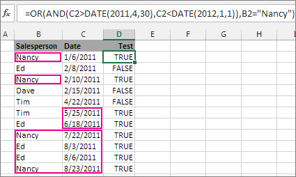
This formula nests the AND function inside the OR function to search for units sold between April 1, 2011 and January 1, 2012, or any units sold by Nancy. You can see it returns True for units sold by Nancy, and also for units sold by Tim and Ed during the dates specified in the formula.
Here’s the formula in a form you can copy and paste. If you want to play with it in a sample workbook, see the end of this article.
Use AND and OR with IF
You can also use AND and OR with the IF function.
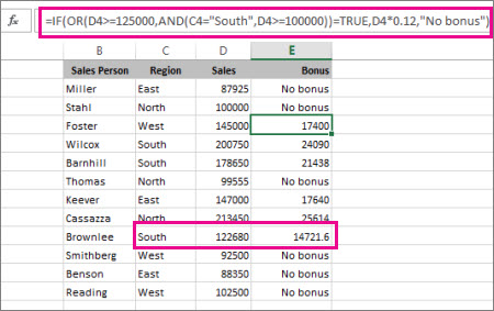
In this example, people don’t earn bonuses until they sell at least $125,000 worth of goods, unless they work in the southern region where the market is smaller. In that case, they qualify for a bonus after $100,000 in sales.
Let’s look a bit deeper. The IF function requires three pieces of data (arguments) to run properly. The first is a logical test, the second is the value you want to see if the test returns True, and the third is the value you want to see if the test returns False. In this example, the OR function and everything nested in it provides the logical test. You can read it as: Look for values greater than or equal to 125,000, unless the value in column C is «South», then look for a value greater than 100,000, and every time both conditions are true, multiply the value by 0.12, the commission amount. Otherwise, display the words «No bonus.»
Sample data
If you want to work with the examples in this article, copy the following table into cell A1 in your own spreadsheet. Be sure to select the whole table, including the heading row.
Источник
Excel IF OR function with formula examples
 by Svetlana Cheusheva, updated on March 16, 2023
The tutorial shows how to write an IF OR statement in Excel to check for various «this OR that» conditions.
IF is one of the most popular Excel functions and very useful on its own. Combined with the logical functions such as AND, OR, and NOT, the IF function has even more value because it allows testing multiple conditions in desired combinations. In this tutorial, we will focus on using IF-and-OR formula in Excel.
IF OR statement in Excel
To evaluate two or more conditions and return one result if any of the conditions is TRUE, and another result if all the conditions are FALSE, embed the OR function in the logical test of IF:
In plain English, the formula’s logic can be formulated as follows: If a cell is «this» OR «that», take one action, if not then do something else.
Here’s is an example of the IF OR formula in the simplest form:
=IF(OR(B2=»delivered», B2=»paid»), «Closed», «Open»)
What the formula says is this: If cell B2 contains «delivered» or «paid», mark the order as «Closed», otherwise «Open». 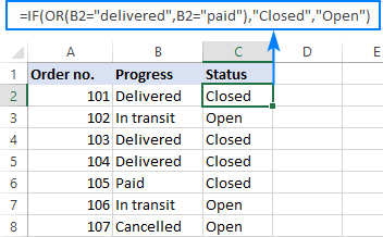
In case you want to return nothing if the logical test evaluates to FALSE, include an empty string («») in the last argument:
=IF(OR(B2=»delivered», B2=»paid»), «Closed», «»)
The same formula can also be written in a more compact form using an array constant:
=IF(OR(B2=<«delivered»,»paid»>), «Closed», «») 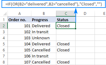
In case the last argument is omitted, the formula will display FALSE when none of the conditions is met.
Note. Please pay attention that an IF OR formula in Excel does not differentiate between lowercase and uppercase characters because the OR function is case-insensitive. In our case, «delivered», «Delivered», and «DELIVERED», are all deemed the same word. If you’d like to distinguish text case, wrap each argument of the OR function into EXACT as shown in this example.
Excel IF OR formula examples
Below you will find a few more examples of using Excel IF and OR functions together that will give you more ideas about what kind of logical tests you could run.
Formula 1. IF with multiple OR conditions
There is no specific limit to the number of OR conditions embedded into an IF formula as long as it is in compliance with the general limitations of Excel:
- In Excel 2007 and higher, up to 255 arguments are allowed, with a total length not exceeding 8,192 characters.
- In Excel 2003 and lower, you can use up to 30 arguments, and a total length shall not exceed 1,024 characters.
As an example, let’s check columns A, B and C for blank cells, and return «Incomplete» if at least one of the 3 cells is blank. The task can be accomplished with the following IF OR function:
And the result will look similar to this: 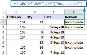
Formula 2. If a cell is this OR that, then calculate
Looking for a formula that can do something more complex than return a predefined text? Just nest another function or arithmetic equation in the value_if_true and/or value_if_false arguments of IF.
Say, you calculate the total amount for an order (Qty. multiplied by Unit price) and you want to apply the 10% discount if either of these conditions is met:
- in B2 is greater than or equal to 10, or
- Unit Price in C2 is greater than or equal to $5.
So, you use the OR function to check both conditions, and if the result is TRUE, decrease the total amount by 10% (B2*C2*0.9), otherwise return the full price (B2*C2):
=IF(OR(B2>=10, C2>=5), B2*C2*0.9, B2*C2)
Additionally, you could use the below formula to explicitly indicate the discounted orders:
The screenshot below shows both formulas in action: 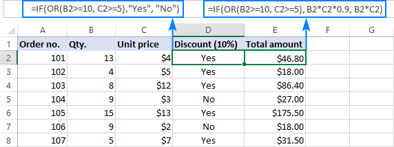
Formula 3. Case-sensitive IF OR formula
As already mentioned, the Excel OR function is case-insensitive by nature. However, your data might be case-sensitive and so you’d want to run case-sensitive OR tests. In this case, perform each individual logical test inside the EXACT function and nest those functions into the OR statement.
In this example, let’s find and mark the order IDs «AA-1» and «BB-1»:
=IF(OR(EXACT(A2, «AA-1»), EXACT(A2, «BB-1»)), «x», «»)
As the result, only two orders IDs where the letters are all capital are marked with «x»; similar IDs such as «aa-1» or «Bb-1» are not flagged: 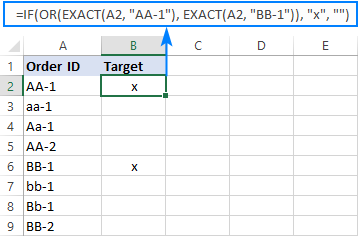
Formula 4. Nested IF OR statements in Excel
In situations when you want to test a few sets of OR criteria and return different values depending on the results of those tests, write an individual IF formula for each set of «this OR that» criteria, and nest those IF’s into each other.
To demonstrate the concept, let’s check the item names in column A and return «Fruit» for Apple or Orange and «Vegetable» for Tomato or Cucumber:
=IF(OR(A2=»apple», A2=»orange»), «Fruit», IF(OR(A2=»tomato», A2=»cucumber»), «Vegetable», «»)) 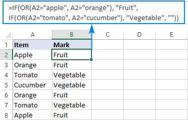
Formula 5. IF AND OR statement
To evaluate various combinations of different conditions, you can do AND as well as OR logical tests within a single formula.
As an example, we are going to flag rows where the item in column A is either Apple or Orange and the quantity in column B is greater than 10:
=IF(AND(OR(A2=»apple»,A2=»orange»), B2>10), «x», «») 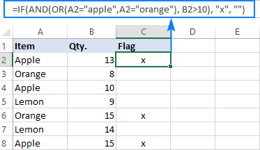
That’s how you use IF and OR functions together. To have a closer look at the formulas discussed in this short tutorial, you are welcome to download our sample Excel IF OR workbook. I thank you for reading and hope to see you on our blog next week!
You may also be interested in
Table of contents
can you help me please.
i have the following IF/OR formula i’m try to build. Basically its looking up a cell for either ME (Meter),IN (Inch) or CM (Centimeter). if ANY of the dimensions are greater than 1.2 (ME), 120(CM) or 47.2 (IN) there is a value of 70. if not, the value is zero.
can you see where i’m going wrong on this
help much appreciated.
Hi!
I do not have your data, so it is difficult to understand your formula and impossible to check it. However, check in the first OR condition: AP3202=»ME»,AP3202>1.2
Hi I am trying to get a formula for this:
-produce the label ‘points if either a reservation’s Total Tour Price exceeds 300 or has more than six(6) persons in the tour party. Otherwise leave the cell blank
I tried but getting it incorrect. Thanks
Hi!
Please re-check the article above since it covers your case.
Please Suggest I have a few criteria
There are 3 column A= Inventory on Website, B= Inventory In Hand and C= reserved qty (B-5)
Need to write a formula where, If A is greater than C then need to correct Website inventory and if C is 0 or less than 5 then update as out of stock and if C is greater than A and greater than 5 then, update inventory
Hi!
The answer to your question can be found in this article: Nested IF in Excel – formula with multiple conditions.
For example:
=IF(A1>C1,»correct», IF(C1 A1,»inventory»,»»)))
This is great article & very helpful,
I am a beginner and tried to correct one of below formula on my own and it takes time.
in C5 I have name of the day like Mon, Tue, Wed etc.
in B11 I have a fruit names like Apple, Banana, Grapes etc.
in C11 I have number of kilo
I tried several combinations of the parentesis as well as AND, NOT functions but no luck.
this is the problem;
— if it is a «Mon» don’t calculate kilos of these fruits.
— if it is not a «Mon» calculate kilos of only these fruits
if is this kind of formula possible for kind of problem? and would you please help on this.
Thank you very much in advance
Hi! Based on your description, it is hard to completely understand your task. However, I’ll try to guess and offer you the following formula:
If you want to calculate the sum for these fruits, use the SUMIFS function. I recommend reading this guide: Excel SUMIFS and SUMIF with multiple criteria – formula examples.
Thank you very much for your reply.
The above formula did not worked thru but I add one more if(..) in the middle and it worked
Thank you very much.
Hi,
Helpfull article!
I have 6 variables in total. Only one variable will actually be found each time and then I would like that specific variable back in text.
*have to use «;» instead of comma’s in my excel.
Doing this now, but not working:
=IF(OR(ISNUMBER(SEARCH(«Var1″;A28));»Var1»);
IF(OR(ISNUMBER(SEARCH(«Var2″;A28));»Var2»);
IF. etc. ))
If you have many conditions try using the IFS function instead of multiple IF:
I hope my advice will help you solve your task.
Hi need help. I would want to automatically get the rates when these combinations are selected. Please see table. Thank you so much in advance.
Service Paper Size Print Color Rate
Print — Plain TEXT Letter Grayscale | B/W 5.00
Print — Plain TEXT A4 Grayscale | B/W 5.00
Print — Plain TEXT Long / Folio Grayscale | B/W 7.00
Print — IMAGE (Half page) Letter Grayscale | B/W 7.00
Print — IMAGE (Half page) A4 Grayscale | B/W 7.00
Print — IMAGE (Half page) Long / Folio Grayscale | B/W 10.00
Print — IMAGE (Half page) Letter Colored 12.00
Print — IMAGE (Half page) A4 Colored 12.00
Print — IMAGE (Half page) Long / Folio Colored 15.00
Print — IMAGE (Full page) Letter Grayscale | B/W 10.00
Print — IMAGE (Full page) A4 Grayscale | B/W 10.00
Print — IMAGE (Full page) Long / Folio Grayscale | B/W 12.00
Print — IMAGE (Full page) Letter Colored 15.00
Print — IMAGE (Full page) A4 Colored 15.00
Print — IMAGE (Full page) Long / Folio Colored 20.00
Print — Digital photo 4R Colored 30.00
Photocopy Letter Grayscale | B/W 5.00
Photocopy Letter Colored 7.00
Photocopy A4 Grayscale | B/W 5.00
Photocopy A4 Colored 7.00
Scan 10.00
addt’l — Editing 3.00
Hello!
You can find the answer to your question in this guide: Extract a substring after the last occurrence of the delimiter
Thank you for this but I am not looking for the delimiter. What I am trying to get is the «RATES». For instance if I input «Print — Plain TEXT» on «SERVICE» then «Long / Folio» on the «PAPER SIZE» then «Grayscale» on «Print colour» it will get me automatically the «RATE» of 7.00..
Hi!
From text: Print — Plain TEXT Long / Folio Grayscale | B/W 7.00 — formula extracts 7.00
If it is not a single text string but several cells, which you did not mention, use these guidelines: Excel INDEX MATCH with multiple criteria.
Hey Alexander Trifuntov ! Thank you so much for the help. Works really great! Awesome! Just as the result I really wanted. 😀
I am trying to sum a range of cells if another range of cells says either yes or no. If yes then sum the cells, if no, then subtract the amount in that cell. Can someone help?
Hi!
You can also find useful information in this article: How to use SUMIF function in Excel with formula examples. I hope it’ll be helpful.
doc_no frm_date to_date missing date
1662450337 01-Apr-22 04-Apr-22
1662450337 05-Apr-22 07-May-22
1662450337 08-May-22 04-Jun-22
1662450337 05-Jun-22 04-Jul-22
1662450337 05-Jul-22 04-Aug-22
1662450337 05-Aug-22 04-Sep-22
1662450337 05-Sep-22 04-Oct-22
Can you please help. i need help with the following
if for example K20= «CH» is not listed in the above formula. is there an add on to this formula to just show K20 as CH
Hope this makes sense.
this is the full formula i’m looking for, but no joy. help would be greatly appreciated
=IF($K20=»DE»,IF($Z20>150,GB 320000),IF($K20=»FR»,IF($Z20>150,GB 320000),IF($K20=»SE»,IF($Z20>150,GB 320000),IF($K20=»ES»,IF($Z20>150,GB 320000),IF($K20=»IE»,IF($Z20>150,GB 320000),IF($K20=»IT»,IF($Z20>150,GB 320000),IF($K20=»DK»,IF($Z20>150,GB 320000),IF($K20=»NL»,IF($Z20>150,GB 320000),IF($K20=»CH»,IF($Z20>0,CH)
Hi!
Add another OR condition as described in the article above.
I am using the following formula, but I am finding examples where the SUM of T to V = 2 in the first argument and it is still returning a Compliant result when it should be Non Compliant for not being = to 3?
Hello!
You are using the logical OR function. If at least one condition is true, the formula returns TRUE.
Simple formula, but I can’t figure out how to use IF, or if it is IF OR or IF AND to nest the ifs.
Column A (Salary) has values ranging from 10 to 100.
I want to indicate in Column B whether the numbers in Column A would be, ’75 and below,’ ’50 and below,’ and ’25 and below.’
I can do the basic =IF(A2 Reply
Hi!
Use nested IF function and this example. This should solve your task.
Thanks for you great works.
I am working on a file with column A containing dropdown list of numbers 100, 200, and 300. The number represents «account department», «legal department» and «sales department» respectively.
How can I make column B dependent on what is chosen on the dropdown list of column A? That is, if 100 is chosen on the dropdown list in column A, I want column B to return «account department» on its own.
Hi!
If you want to check if multiple conditions are true, use a nested IF function.
I would like to calculate a sum of products, but with a pricing break.
1st item= $50, 2nd item onwards = $70 each
Let’s say if A buys 3 products, he will have to pay $50 for the first product, for the other 2 items, he will have to pay $70 each.
How could I create a formula for this problem? Hope you could assist me, it’ll be a great help
Thank you in advance
Hi!
Use the IF function to calculate the sum for values greater than zero.
The formula below will do the trick for you:
I’m trying to use IF to show «ok» or «out of balance» if a value is over or under by more than 5%.
Cell C20 has a value of 700
Cell C21 has a value of 650
My formula for D20 is =C20-C21 giving a value of 50
My formula for D20 is =IF(D20 Reply
Hi!
To ignore what is a positive or negative number, use the ABS function —
This should solve your task.
Cell I2=»Any Text», J2=»Blank Text,K2=»Blank Text,L2=»Blank Text,
than need answer in Cell M=»Any Text»
Blank Text = Blank Cell
one column have any text and other column have no text, I want to type text only automatically
Hi!
You can merge cell values using the CONCATENATE function as described in this article: Combine text strings, cells and columns.
Is there a syntax error with this formula? I’m getting #Name. Likewise with this formula,
Hi!
When you copy a formula from a website page, change the slash quotes ” to straight quotes «.
Hi there-
I’m trying to code blood pressure according to JNC 7 criteria for normal/prehypertension/stage 1/stage 2 categories. i have different collumns for «systolic» and «diastolic» blood pressure numbers. A blood pressure can qualify for prehypertension, for example, if the systolic OR the diastolic numbers qualify. Here is what I have — can you help me figure out why it’s not working?
=IF(OR(G10 > 159,H10 > 99),»2″,IF(OR(G10 > 139,H10 > 89),»1″,IF(OR(G10 > 119,H10 > 79)»PRE»,IF(G10 Reply
Hi!
I can’t see your data and therefore can’t tell what doesn’t work in the IF function with multiple conditions. But a comma was missing in the formula.
=IF(OR(G10 > 159,H10 > 99),»2″,IF(OR(G10 > 139,H10 > 89),»1″,IF(OR(G10 > 119,H10 > 79),»PRE»,IF(G10 Reply
Trying to combine these two IF statements into one IF OR statement:
Hi1
What you want to do is not possible. These formulas use different values and are not connected in any way.Please re-check the article above.
What is the best way to combine the two following statements. Combing is where I seem to have problems.
=IF(AND(K2=»Not Urgent»),IF(N23, «Fail»)))
Hi!
Based on your description, it is hard to completely understand your task. IF(N21,”Fail”) — doesn’t make sense. However, I’ll try to guess and offer you the following formula:
i have customers data in excel how create customer wise statement a period of year or month
Hi!
The information you provided is not enough to understand your case and give you any advice. However, I can assume that you can select data about the customer using the FILTER function. The following tutorial should help: Excel FILTER function — dynamic filtering with formulas.
I could not get this formula to work. Could you help me identify where could be the error? It always gives a #VALUE! result.
Hi!
Your formula is so big that it is impossible to understand it. It’s not clear what you want to do. However, keep in mind that such a formula always returns an array of values.
See the result of this formula.
“Gopal informed other students if you score 20 marks in end term exam OR 60 marks in total in
subject then you PASS otherwise FAIL.” write an excel command.
I need help,
I have this scenario where Agent 1 has a ceiling of 500, Agent 2 has 250 and Agent 3 has 150.
If at anytime any of the agents pay goes above the ceiling, then 10% is calculated on the ceiling if the pay is below the ceiling then the 10% is calculated on that amount
How do i use IF statement to achieve this in Excel
Hello!
I recommend reading this guide: Nested IF in Excel – formula with multiple conditions.
If I understand your task correctly, the following formula should work for you:
=IF(A1=»Agent 1″,IF(B1>500,500*10%,B1*10%),IF(A1=»Agent 2″,IF(B1>250,250*10%,B1*10%),IF(A1=»Agent 3″,IF(B1>150,150*10%,B1*10%))))
This works. Thank you
Hello,
Is there a way to combine two formulas below:
=IF(B63=TRUE; (G63)-(F63*1,21*D63); 0)
=IF(B63=TRUE; (G63)-(F63*1,21*D63); 0)
Tried this way, but it’s not working:
=IF(B63=TRUE; (G63)-(F63*1,21*D63); 0); OR(=IF(B63=TRUE; (G63)-(F63*1,21*D63); 0))
Thank You for Your time!
Sorry, mistake! I meant:
=IF(B63=TRUE; (G63)-(F63*1,21*D63); 0)
=IF(H63=»Paid»; (G63)-(F63*1,21*D63); 0
Tried this way, but it’s not working:
=IF(B63=TRUE; (G63)-(F63*1,21*D63); 0); OR(=IF(H63=»Paid»; (G63)-(F63*1,21*D63); 0))
Hi!
I think you have not read the article very carefully. There is an answer to your question.
I really appreciate Your answer! Thank You!
How To Extract Unique Values or Duplicate Names and sort (A-Z) Based On Criteria In Excel? Using index or match.
Sl No# Location Name score
1 Mumbai Rohit 93
2 Mumbai Sachin 93
3 Gujrat Suresh Raina 90
4 Ranchi M.S Dhoni 85
5 Ranchi Sorabh Tiwari 85
Hello!
How to extract unique values using INDEX + MATCH functions, read this tutorial.
Your examples helped me find a solution — thanks for posting this page.
Please check to see if the following is an error in the section «IF OR statement in Excel» where you state the lines below [in brackets like those enclosing this phrase to avoid confusion if I used double quotes]:
[ Here’s is an example of the IF OR formula in the simplest form:
=IF(OR(B2=»delivered», B2=»paid»), «Closed», «Open»)
What the formula says is this: If cell B2 contains «delivered» or «cancelled», mark the order as «Closed», otherwise «Open». ]
However, as I read the formula, it indicates that if cell B2 contains «delivered» or «paid» (not «cancelled») then the order will be marked as «Closed». If you look at the screen shot, the row containing «Cancelled» shows a Status of «Open», not «Closed» as your explanation states it will. Please clarify for your readers.
Of course, it is «paid», not «cancelled». Thank you for pointing that out, fixed!
I am trying to say that if One Cell = this amount add / subtract a Certain amount.
Can this be done??
EX: =IF(D6/7=E6,G6) OR (D6/7=E6,H6) OR (D6/7=E6,I6) OR (D6/7=E6,J6) OR (D6/7=E6,K6)
Hi!
Sorry, I cannot understand your formula
=IF(AND(A2=»VISHAL», B2=»HP», C2=610), «6», «10»), IF(AND(A2=»VISHAL», B2=»HP», C2=2310), «15», «20»)
WILL THIS WORK.
I NEED TO ENTER MULTIPLE RESULT IN A SINGLE CELL, FROM DIFFERENT CONDITIONS.
Hello!
Your conditions contradict each other. For example, if A2 = ”VISHAL”, B2 = ”HP”, C2 = 900 then the first condition will return 10, and the second — 20.
This isn’t working. What am I doing incorrectly?
=IF((OR(E2=Daily, E2=Weekly)), Next Shift, ENTER DATE)
Column E indicates if a project is due daily or weekly. Column F would ideally calculate today+1 for daily or today+8 days for weekly.
Hi,
You must enclose text values in quotation marks, such as «Weekly».
What is «Next Shift, ENTER DATE»?
Based on your description, it is hard to completely understand your task. However, I’ll try to guess and offer you the following formula:
Hope this is what you need.
I got it! thank you. 🙂
Hi.. need help.
i have date today and start date, to calculate the case age but another column is the status of the case, close or open.. so the logic will be.. calculate the case age if the case is still open..
thank you in advance.
I got this formula: =IF(OR(C2=»Closed»,»—«),(SUM(A2-B2)))
but..
it’s working but the other way around. it calculates the age if the case is marked as «Closed».
Hello!
In the condition of the IF function, write down the check that the case is open. If the condition is met, calculate the age using the DATEDIF function.
Hope you’ll find this information helpful.
Hi, I would like to know a formula to show if something if greater than or less than a number to show a figure for example
11 years service — if the years service is more than 10 to show 2, if it is less than 10 but more than 5 to show 1 and if it is less than 5 to show 0.
hope this makes sense.
Hello!
I hope you have studied the recommendations in the tutorial above. It contains answers to your question.
there are some proble with me in excell example
=if(a1 Reply
Please I need your help how can I come up with the formula for this
45000 =0%
5000=15%
Next 2950000=30%
Excess 3000000=35%
Hello!
A similar question has already been asked many times on our blog. I think this answer will be helpful.
I need some help in constructing the formula to this:
I need to derive a result(column title) if ALW(column title) is 1.56 and up its Oversize, if ALW is 1.20-1.55 its Goodsize, if ALW is 1.10-1.19 its Undersize, if ALW is 1.0-1.09 its Offsize, and if ALW is below 1.0 its Runts
Hello!
I’m sorry but your task is not entirely clear to me.
What is the column title? In Excel and other spreadsheet applications, the column header is the colored row of letters used to identify each columnwithin the sheet, or workbook. Column title is a letter.
If your question is about an Excel cell —
=IF(A1>=1.56,»Oversize», IF(A1>=1.2,»Goodsize», IF(A1>=1.1,»Undersize», IF(A1>=1,»Offsize», «Runts» ))))
i need a formula like ( date of joinin — current date less than 365 days then the answer should be 0
Hello!
How to use Excel IF function with dates read in this article.
Hi,
I am trying to do the following if statements with the last if statement to add on an additional 1 week if P13 = «U» but I can’t get this to work. Any help would be welcomed.
=IF(AND(O131,O133,O135),4,IF(AND(P13=»U»,2),TRUE)))))
Hi,
I am trying to do the following if statements with the last if statement to add on an additional 1 week if P13 = «U» but I can’t get this to work. Any help would be welcomed.
=IF(AND(O131,O133,O135),4,IF(AND(P13=»U»,2),TRUE))))).
Thanks so much.
Hello Joanne!
I’m sorry but your task is not entirely clear to me.
Please describe your problem in more detail. Include an example of the source data and the result you want to get. It’ll help me understand your request better and find a solution for you. Thank you.
IF(A1=»DELIVERY»,THEN C1(CELL NO)*.020%,IF NO C1*.004% I NEED CORRECT FORMULA
How do I write the formula for. If either Cell A1 or Cell D1 contains a term, say «ENGLISH», then the consequent grade of ENGLISH from the C1 or F1 should be filled in cell G1.
Is it possible?
Hello Michael!
If I got you right, the formula below will help you with your task:
I hope it’ll be helpful.
I NEED A FORMULA FOR CELL F45
IF CELL E45 = «PA1» THEN CELL F45= .85 AND IF CELL E45 = PA2 THEN CELL F45 READS .95 AND IF CELL = E45 — CB1 THEN F45 = .99
Trying to write a formula that picks out the word grapefruit from D14 or the word recorder from D14 and gives a zero.. if those words aren’t found then F14-E14. The formula works for just Grapefruit but when I add in the Or and Recorder it doesn’t. What am I writing wrong? It’s telling me to many arguments.
=If(Or(Is number(Search(«Grapefruit»‘D14,(Is number(Search(«Recorder»,D14),0,F14-E14))
Can I not make cell to cell comparison with if/or? Here is the formula I am using.
=IF(OR(D3 Reply
Here is the formula I used after reviewing the responses to other questions on this forum. New formula works.
=IF(D3 Reply
Hi Sam,
Your original formula would work as well. You just had to move the other bracket to close off the or( function.
=IF(OR(D3 Reply
Can you help me on the error in this formula. =IF(ISNUMBER($AH15),ANDIF($AH15>150,(» High Random Blood Sugar «&$AH15&» Mg.%. «, «»)&» «&IF($AH15>150,»Urine Sugar «&$AI15&». «, «»),(«»)
AH15 is Number or Text «ND» i.e. Not Done.
Thank you.
=IF(OR(ISNUMBER($AH15),$AH15=»ND»),IF($AH15>150,»High Random Blood Sugar»&$AH15&»Mg.%.»,»»)&» «&IF($AH15>150,»Urine Sugar»&» «&$AI15&».»,»»),»»)
The above formula seems to work for me.
I have a price range for warranty coverage. I need to see when sales either sold the item over or under the range for a warranty package. For example:
Min Product $ Range Max Product $ Range Product $ Sold
1000 1499.99 269.00
300 599.99 1049.00
1000 1499.99 578.00
600 799.99 1456.00
I need a formula that tells me if the product sold for $269.00 was «oversold» or «undersold» contract range? I tried =if(or(c1=B2,»oversold»))
It doesn’t work. What am I doing wrong?
A = Min / B = Max / C = Sold
=IF(C1B1,»OVERSOLD»,»»)
Something is wrong with the formula not being posted properly.
=IF(C1B1,»OVERSOLD»,»»)
It should be:
=IF(C1 less than A1,»UNDERSOLD»,IF(C1 greater than B1,»OVERSOLD»,»»)
Hello,
I want to write a formula to write C1 as:
1 if A1>10 or B1>20
2 if 7 3 if 4 4 if 1 5 if A1 Reply
I have student totals,I want to apply comments, 400 and above should have good performance, 300-400 should have fair performance, below 300 should have poor performance,the cell for total is I
I need a formula in google spreadsheet that will:
+1 when the value is >=5,
+2 when the value is >=10,
+3 when the value is >=15,
+4 when the value is >=20,
+5 when the value is >=25
The formula I am currently using is:
=IF(F7>=5,H7+1,IF(F7>=10,H7+2,IF(F7>=15,H7+3,IF(F7>=20,H7+4,H7))))
This formula is working for the +1 when the value is >=5, but when the value is >=10, it is still adding +1.
Please Help!
You see, your first condition fits to all other conditions as well — the value is greater than 5. You need to limit each condition and check, for example, if the number is not only greater than or equal to 5 but also less than 10.
Your formula for spreadsheets should look like this:
=IF(AND(F7>=5,F7 =10,F7 =15,F7 =20,H7+4, H7))))
You will find the info about the IF function in Google Sheets in this post.
I have 2 columns, work email(D2) & personal email(E2). I am trying to create a formula in a new field (preferred email) that says if D2 is blank use E2 (if there is a value) or if E2 is blank use D2 or leave blank. Is this possible?
Hi,
If I get it right, your task is as follows: if a cell in Column D contains an email address, a formula is to bring it; if not, it should bring an email address from a cell in Column E; if both cells are empty, the formula has to bring nothing. I hope you do not mind lengthy formulas:
=IFS(OR(AND(N(ISBLANK(D2))=0, N(ISBLANK(E2))=0), AND(N(ISBLANK(D2))=0, N(ISBLANK(E2))=1)), D2, AND(N(ISBLANK(D2))=1, N(ISBLANK(E2))=0), E2, AND(N(ISBLANK(D2))=1, N(ISBLANK(E2))=1), «»)
If you love compact formulas, use this one 🙂
Someone please help me, i cant get this to work
In column C I enter one of 7 names.
Depending on the name I want different results in column N
So
If the name is
1 — Andy Black the result should be 400
2 — Mr Jet, Nina Sven or Mike Young the result should be 600
3 — Dr Joe, Miss Adams or Neil Foe the result should be 800
4 — Ms Hard the result should be 1000
5 — Mr Woo the result should be 1200
Which formula do I use to solve this?
Hi Björne,
The following formula suggests itself:
=IFS(C2=»Andy Black», 400, OR(C2=»Mr Jet», C2=»Nina Sven», C2=»Mike Young»), 600, OR(C2=»Dr Joe», C2=»Miss Adams», C2=»Neil Foe»), 800, C2=»Ms Hard», 1000, C2=»Mr Woo», 1200)
Formula 2. If a cell is this OR that, then calculate
=IF(OR(D3>0,D390,D3180,D3270,D30,D390,D3180,D3270,D3 Reply
I am looking for the correct formula to use to return the greatest of two values. For example, if Q3 (5.89) is greater than R3 (7.452), I want S3 to show R3 value (7.452). If Q17 (28.86) is greater than R17 (3.105), I want S17 to show Q17 value (28.86).
Hi Jwalker,
I hope that your task may be expressed in the following way: if the value in Cell R3 is less than the value in Cell Q3, the value from Cell Q3 is needed; if the value in Cell R3 is more than the value in Cell Q3, the value from Cell R3 is needed. If so, here is the formula you could apply:
I need to validate customer order to ensure it is not less than minimum order value(MOV) and not less than minimum order qty. We validated order value on one column, filter out the order lines with order value lower than MOV and then validated order qty on another column. Is there shortcut to have all the validation performed under single column with a sophisticated nested if function?
hi everyone,
how can i formulate this one?
if >=6 : full assistance
if =4 or 5 : half assistance
if Reply
Hi Farzaneh,
I hope the following formula will do the job:
=IFS(D2 =6, «full assistance»)
So how would I do this? If cell A1 is equal to 10, I want to multiply B1 by ten, but if A1 is equal to 25 I want to multiply B1 by four, but if A1 is equal to 50 I want to multiply B1 by 2.
Thanks in advance!
Hi Marty,
I think that both the IF function and the IFS function may help you with your task. Please choose whatever you like:
=IF(A1=10, B1*10, IF(A1=25, B1*4, IF(A1=50 ,B1*2)))
=IFS(A1=10, B1*10, A1=25, B1*4, A1=50, B1*2)
Hi all
I want to differentiate the cell values into the crores, Lakh, Thousand, Hundred, Tens, Units
Example : —
123456789
12 Crores 24 Lakh 56 Thousand 7 Hundred 89
So how will i do can anyone here who can help me
Hi, Hoping someone can help.
I’m trying to write a formula using the IF, AND, or OR function but can’t get the formula correct. It should be simple, really.
The conditions are;
If the SUM of Cells E4:G4 = between 10 and 15, then Cell G14 = 25
If the SUM of Cells E4:G4 is greater than or equal to 15, then Cell G14 = 50
Then there’s one other result that I’m trying to achieve (in a separate cell but a similar formula)
If the SUM of Cells E4:P4 = between 400 and 600, then Cell P15 = 10
If the SUM of Cells E4:P4 is greater than or equal to 600, then Cell P15 = 20
I can’t work out what I’m doing wrong, I wont paste what formulas i currently have to avoid causing a case of mass confusion.
THANKS IN ADVANCE
Completely butchered the original answer. This one should work.
I am trying to evaluate if the first date is a weekend or the time is after 5pm.
Each works on its own but is not working when combines with the OR
I am getting #NAME?
=IF(OR(WEEKEND(E2,2)>5,K19>TIME(17,0,0)),»OT», «REG»)
Apparently I just needed to retype and press the keyboard harder:) it worked the 50th time I typed it I don’t know why as it looks exactly the same. But for now I will move on.
If F34 value = «Dealer», then used values Column K OR
If F34 value = «Trade», then use values Column M OR
If F34 value = «End User», then use values Column
If I want to reference three cells, what’s the formula? (i.e =IF(F113-«x»,(J126)),=IF(G113-«x»,(K126)),=IF(H113-«x»,(K126))
H126 want to be the value of one of three cells depending the selection of another value in three cells
Thanks in advance
I need little help to construct formula from below pseudo code.
If <
customer = private AND account_status = active AND account_open_date >23-June-2006
THAN
If <
risk = high
THAN
Last Review date = 1st review date + 6 Months
>
Else If <
risk = medium
THAN
Last Review date = 1st review date + 12 Months
>
Else If <
risk = low
THAN
Last Review date = 1st review date + 12 Months
>
Else <
last review date = 24-June-2006
>
>
If <
customer = govt AND account_open_date 23-June-2006
THAN
If <
risk = high
THAN
Last Review date = 1st review date + 6 Months
>
Else If <
risk = medium
THAN
Last Review date = 1st review date + 12 Months
>
Else If <
risk = low
THAN
Last Review date = 1st review date + 12 Months
>
>
I need the response in column D , labeled «link», to substitute the number of the column with the actual entry in that column of the row. The desired results, column E, are in the «want» column. Any thoughts?
1 2 3 LINK WANT
J18.9 A41.9 1 J18.9
R41.82 E86.0 E43 2 E86.0
G20 R26.89 G30.9 1,3 G20, G30.9
Thanks for your teach, but i think that is better to use brackets, especially if B2 can have several values
=IF(OR(B2=»delivered», B2=»paid»), «Closed», «Open»)
I agree, this makes the formula more compact. Thanks for the tip!
Hope someone could help me. Trying to figure out my formula. I need to combine if, and & or using text logic. It’s quite simple but my formula can’t capture the correct results. Apparently I use the If and AND and it captures but my вЂвЂ™Not Applicable’’ logic won’t work. рџ©
Here’s my formula for now
If(AND(s2=“Cleared”, t2=“Requested”, t2=“Not Applicable”), “Completed”, “Incomplete”)
FYI I used more than 10 columns. What I’m trying to capture is that some of my values in column has a “NOT APPLICABLE” value.
Thank you in advance.
Hi! Cell T2 cannot have 2 values at the same time.
Hi. Can you help me. i have the following. Column Q is a sum of hours for operations. Column Y is my set hour reset. Y2 Starts at 120 hours and ends at Y23 at 2640 hours. increments are in 120 hours.
In Columm Q i have the following formula =Sum(K3+Q2). on R3 i want to add a formula to do the following.
If cell Q3 is 120240 then subtract Q3-$Y$2, or if Q3 is 241360 then Subtract Q3-$Y$3, or if Q3 is 361480 then subtract Q3-$Y$4, if false then add K3+Q2
Whats the best way for me to write it.
i manage to write a formula but it turns the cell in Column R when ever the statement is true «true».
Very good article, thanks for sharing, Keep up the good work!
please assist
if A>=2(Fail),if b>=3(Fail),but if A:B>=3(Fail)
How do i get this into one fomula
So how would I do this? If cell A1 is equal to 10, I want to multiply B1 by ten, but if A1 is equal to 25 I want to multiply B1 by four, but if A1 is equal to 50 I want to multiply B1 by 2.
Thanks in advance!
Ooops, sorry, didn’t mean to reply to your question with my question.
Copyright © 2003 – 2023 Office Data Apps sp. z o.o. All rights reserved.
Microsoft and the Office logos are trademarks or registered trademarks of Microsoft Corporation. Google Chrome is a trademark of Google LLC.
Источник
In this article, we will learn to apply multiple conditions in a single formula using OR and AND function with the IF function.
IF function in Excel is used to check the condition and returns value on the basis of it.
Syntax:
=IF(Logic_test, [Value_if True], [Value_if_False])
OR function works on logic_test. It helps you run multiple conditions in Excel. If any one of them is True, OR function returns True else False.
Syntax:
=OR( Logic_test 1, [logic_test 2], ..)
AND function works on logic_test. It helps you run multiple conditions in Excel. If every one of them is True, then only AND function returns True else False.
Syntax:
=AND( Logic_test 1, [logic_test 2], ..)
First we will use IF with OR function.
Let’s get this by an example here.
We have a list of months and need to know in which quarter it lay.
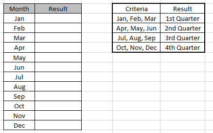
Use the formula to match the quarter of the months
Formula:
=IF(OR(A4=”Jan”,A4=”Feb”,A4=”Mar”),”1st
Quarter”,IF(OR(A4=”Apr”,A4=”May”,A4=”Jun”),”2nd
Quarter”,IF(OR(A4=”Jul”,A4=”Aug”,A4=”Sep”),”3rd
Quarter”,IF(OR(A4=”Oct”,A4=”Nov”,A4=”Dec”),”4th Quarter”))))
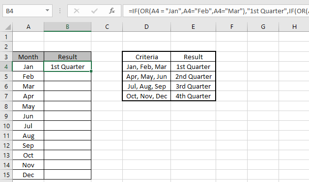
Copy the formula in other cells, select the cells taking the first cell where the formula is already applied, use shortcut key Ctrl +D
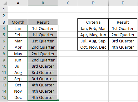
We got the result.
You can use IF and OR function to meet multiple conditions in a single formula.
Now we will use IF with AND function in Excel.
Let’s get this by an example here.
We have a list of Scores and We need to know under which criteria it lay.
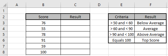
Use the formula to match the criteria
Formula:
=IF(AND(B3 > 50, B3 < 60), «Below Average»,IF(AND(B3 > 60, B3 < 90),»Average»,IF(AND(B3 > 90,B3< 100),»Above Average»,»Top Score»)))

Copy the formula in other cells, select the cells taking the first cell where the formula is already applied, use shortcut key Ctrl + D
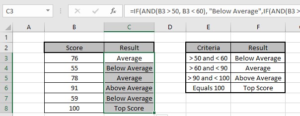
We got the Results corresponding to the Scores.
You can use IF and AND function to meet multiple conditions in a single formula.
Hope you understood IF, AND and OR function in Excel 2016. Find more articles on Logic_test here. Please share your query below in the comment box. We will assist you.
Nesting functions in Excel refers to placing one function inside another. The nested function acts as one of the main function’s arguments. The AND, OR, and IF functions are some of Excel’s better known logical functions that are commonly used together.
Instructions in this article apply to Excel 2019, 2016, 2013, 2010, 2007; Excel for Microsoft 365, Excel Online, and Excel for Mac.
Build the Excel IF Statement
When using the IF, AND, and OR functions, one or all of the conditions must be true for the function to return a TRUE response. If not, the function returns FALSE as a value.
For the OR function (see row 2 in the image below), if one of these conditions is true, the function returns a value of TRUE. For the AND function (see row 3), all three conditions must be true for the function to returns a value of TRUE.
In the image below, rows 4 to 6 contain formulas where the AND and OR functions are nested inside the IF function.
When the AND and OR functions are combined with the IF function, the resulting formula has much greater capabilities.
In this example, three conditions are tested by the formulas in rows 2 and 3:
- Is the value in cell A2 less than 50?
- Is the value in cell A3 not equal to 75?
- Is the value in cell A4 greater than or equal to 100?
Also, in all of the examples, the nested function acts as the IF function’s first argument. This first element is known as the Logical_test argument.
=IF(OR(A2<50,A3<>75,A4>=100),"Data Correct","Data Error")
=IF(AND(A2<50,A3<>75,A4>=100),1000,TODAY())
Change the Formula’s Output
In all formulas in rows 4 to 6, the AND and OR functions are identical to their counterparts in rows 2 and 3 in that they test the data in cells A2 to A4 to see if it meets the required condition.
The IF function is used to control the formula’s output based on what is entered for the function’s second and third arguments. Examples of this output can be text as seen in row 4, a number as seen in row 5, the output from the formula, or a blank cell.
In the case of the IF/AND formula in cell B5, since not all three cells in the range A2 to A4 are true — the value in cell A4 is not greater than or equal to 100 — the AND function returns a FALSE value. The IF function uses this value and returns its Value_if_false argument — the current date supplied by the TODAY function.
On the other hand, the IF/OR formula in row four returns the text statement Data Correct for one of two reasons:
-
The OR value has returned a TRUE value — the value in cell A3 does not equal 75.
-
The IF function then used this result to return its Value_if_false argument: Data Correct.
Use the IF Statement in Excel
The next steps cover how to enter the IF/OR formula located in cell B4 from the example. These same steps can be used to enter any of the IF formulas in these examples.
There are two ways to enter formulas in Excel. Either type the formula in the Formula Bar or use the Function Arguments dialog box. The dialog box takes care of the syntax such as placing comma separators between arguments and surrounding text entries in quotation marks.
The steps used to enter the IF/OR formula in cell B4 are as follows:
-
Select cell B4 to make it the active cell.
-
On the ribbon, go to Formulas.
-
Select Logical to open the function dropdown list.
-
Choose IF in the list to open the Function Arguments dialog box.
-
Place the cursor in the Logical_test text box.
-
Enter the complete OR function:
OR(A2<50,A3<>75,A4>=100)
-
Place the cursor in the Value_if_true text box.
-
Type Data Correct.
-
Place the cursor in the Value_if_false text box.
-
Type Data Error.
-
Select OK to complete the function.
-
The formula displays the Value_if_true argument of Data Correct.
-
Select cell B4 to see the complete function in the formula bar above the worksheet.
Thanks for letting us know!
Get the Latest Tech News Delivered Every Day
Subscribe