If one value is true excel

IF function

The IF function is one of the most popular functions in Excel, and it allows you to make logical comparisons between a value and what you expect.

So an IF statement can have two results. The first result is if your comparison is True, the second if your comparison is False.

For example, =IF(C2=”Yes”,1,2) says IF(C2 = Yes, then return a 1, otherwise return a 2).

Use the IF function, one of the logical functions, to return one value if a condition is true and another value if it’s false.

IF(logical_test, value_if_true, [value_if_false])

For example:

• =IF(A2>B2,»Over Budget»,»OK»)

• =IF(A2=B2,B4-A4,»»)

Argument name	Description
logical_test    (required)	The condition you want to test.
value_if_true    (required)	The value that you want returned if the result of logical_test is TRUE.
value_if_false    (optional)	The value that you want returned if the result of logical_test is FALSE.

Simple IF examples

• =IF(C2=”Yes”,1,2)

In the above example, cell D2 says: IF(C2 = Yes, then return a 1, otherwise return a 2)

• =IF(C2=1,”Yes”,”No”)

In this example, the formula in cell D2 says: IF(C2 = 1, then return Yes, otherwise return No)As you see, the IF function can be used to evaluate both text and values. It can also be used to evaluate errors. You are not limited to only checking if one thing is equal to another and returning a single result, you can also use mathematical operators and perform additional calculations depending on your criteria. You can also nest multiple IF functions together in order to perform multiple comparisons.

• =IF(C2>B2,”Over Budget”,”Within Budget”)

In the above example, the IF function in D2 is saying IF(C2 Is Greater Than B2, then return “Over Budget”, otherwise return “Within Budget”)

• =IF(C2>B2,C2-B2,0)

In the above illustration, instead of returning a text result, we are going to return a mathematical calculation. So the formula in E2 is saying IF(Actual is Greater than Budgeted, then Subtract the Budgeted amount from the Actual amount, otherwise return nothing).

• =IF(E7=”Yes”,F5*0.0825,0)

In this example, the formula in F7 is saying IF(E7 = “Yes”, then calculate the Total Amount in F5 * 8.25%, otherwise no Sales Tax is due so return 0)

Note: If you are going to use text in formulas, you need to wrap the text in quotes (e.g. “Text”). The only exception to that is using TRUE or FALSE, which Excel automatically understands.

Common problems

Problem	What went wrong
0 (zero) in cell	There was no argument for either value_if_true or value_if_False arguments. To see the right value returned, add argument text to the two arguments, or add TRUE or FALSE to the argument.
#NAME? in cell	This usually means that the formula is misspelled.

Need more help?

You can always ask an expert in the Excel Tech Community or get support in the Answers community.

See Also

IF function — nested formulas and avoiding pitfalls

IFS function

Using IF with AND, OR and NOT functions

COUNTIF function

How to avoid broken formulas

Overview of formulas in Excel

Функция ЕСЛИ в Excel — это отличный инструмент для проверки условий на ИСТИНУ или ЛОЖЬ. Если значения ваших расчетов равны заданным параметрам функции как ИСТИНА, то она возвращает одно значение, если ЛОЖЬ, то другое.

Что возвращает функция

Заданное вами значение при выполнении двух условий ИСТИНА или ЛОЖЬ.

Синтаксис

=IF(logical_test, [value_if_true], [value_if_false]) — английская версия

=ЕСЛИ(лог_выражение; [значение_если_истина]; [значение_если_ложь]) — русская версия

Аргументы функции

• logical_test (лог_выражение) — это условие, которое вы хотите протестировать. Этот аргумент функции должен быть логичным и определяемым как ЛОЖЬ или ИСТИНА. Аргументом может быть как статичное значение, так и результат функции, вычисления;
• [value_if_true] ([значение_если_истина]) — (не обязательно) — это то значение, которое возвращает функция. Оно будет отображено в случае, если значение которое вы тестируете соответствует условию ИСТИНА;
• [value_if_false] ([значение_если_ложь]) — (не обязательно) — это то значение, которое возвращает функция. Оно будет отображено в случае, если условие, которое вы тестируете соответствует условию ЛОЖЬ.

Дополнительная информация

• В функции ЕСЛИ может быть протестировано 64 условий за один раз;
• Если какой-либо из аргументов функции является массивом — оценивается каждый элемент массива;
• Если вы не укажете условие аргумента FALSE (ЛОЖЬ) value_if_false (значение_если_ложь) в функции, т.е. после аргумента value_if_true (значение_если_истина) есть только запятая (точка с запятой), функция вернет значение “0”, если результат вычисления функции будет равен FALSE (ЛОЖЬ).
  На примере ниже, формула =IF(A1> 20,”Разрешить”) или =ЕСЛИ(A1>20;»Разрешить») , где value_if_false (значение_если_ложь) не указано, однако аргумент value_if_true (значение_если_истина) по-прежнему следует через запятую. Функция вернет “0” всякий раз, когда проверяемое условие не будет соответствовать условиям TRUE (ИСТИНА).
  
  |
• Если вы не укажете условие аргумента TRUE(ИСТИНА) (value_if_true (значение_если_истина)) в функции, т.е. условие указано только для аргумента value_if_false (значение_если_ложь), то формула вернет значение “0”, если результат вычисления функции будет равен TRUE (ИСТИНА);
  На примере ниже формула равна =IF (A1>20;«Отказать») или =ЕСЛИ(A1>20;»Отказать»), где аргумент value_if_true (значение_если_истина) не указан, формула будет возвращать “0” всякий раз, когда условие соответствует TRUE (ИСТИНА).

Функция Если в Excel примеры с несколькими условиями

Пример 1. Проверяем простое числовое условие с помощью функции IF (ЕСЛИ)

При использовании функции ЕСЛИ в Excel, вы можете использовать различные операторы для проверки состояния. Вот список операторов, которые вы можете использовать:

Ниже приведен простой пример использования функции при расчете оценок студентов. Если сумма баллов больше или равна «35», то формула возвращает “Сдал”, иначе возвращается “Не сдал”.

Пример 2. Использование вложенной функции IF (ЕСЛИ) для проверки условия выражения

Функция может принимать до 64 условий одновременно. Несмотря на то, что создавать длинные вложенные функции нецелесообразно, то в редких случаях вы можете создать формулу, которая множество условий последовательно.

В приведенном ниже примере мы проверяем два условия.

• Первое условие проверяет, сумму баллов не меньше ли она чем 35 баллов. Если это ИСТИНА, то функция вернет “Не сдал”;
• В случае, если первое условие — ЛОЖЬ, и сумма баллов больше 35, то функция проверяет второе условие. В случае если сумма баллов больше или равна 75. Если это правда, то функция возвращает значение “Отлично”, в других случаях функция возвращает “Сдал”.
  

Пример 3. Вычисляем сумму комиссии с продаж с помощью функции IF (ЕСЛИ) в Excel

Функция позволяет выполнять вычисления с числами. Хороший пример использования — расчет комиссии продаж для торгового представителя.

В приведенном ниже примере, торговый представитель по продажам:

• не получает комиссионных, если объем продаж меньше 50 тыс;
• получает комиссию в размере 2%, если продажи между 50-100 тыс
• получает 4% комиссионных, если объем продаж превышает 100 тыс.

Рассчитать размер комиссионных для торгового агента можно по следующей формуле:

=IF(B2<50,0,IF(B2<100,B2*2%,B2*4%)) — английская версия

=ЕСЛИ(B2<50;0;ЕСЛИ(B2<100;B2*2%;B2*4%)) — русская версия

В формуле, использованной в примере выше, вычисление суммы комиссионных выполняется в самой функции ЕСЛИ. Если объем продаж находится между 50-100K, то формула возвращает B2 * 2%, что составляет 2% комиссии в зависимости от объема продажи.

Пример 4. Используем логические операторы (AND/OR) (И/ИЛИ) в функции IF (ЕСЛИ) в Excel

Вы можете использовать логические операторы (AND/OR) (И/ИЛИ) внутри функции для одновременного тестирования нескольких условий.

Например, предположим, что вы должны выбрать студентов для стипендий, основываясь на оценках и посещаемости. В приведенном ниже примере учащийся имеет право на участие только в том случае, если он набрал более 80 баллов и имеет посещаемость более 80%.

Вы можете использовать функцию AND (И) вместе с функцией IF (ЕСЛИ), чтобы сначала проверить, выполняются ли оба эти условия или нет. Если условия соблюдены, функция возвращает “Имеет право”, в противном случае она возвращает “Не имеет право”.

Формула для этого расчета:

=IF(AND(B2>80,C2>80%),”Да”,”Нет”) — английская версия

=ЕСЛИ(И(B2>80;C2>80%);»Да»;»Нет») — русская версия

Пример 5. Преобразуем ошибки в значения “0” с помощью функции IF (ЕСЛИ)

С помощью этой функции вы также можете убирать ячейки содержащие ошибки. Вы можете преобразовать значения ошибок в пробелы или нули или любое другое значение.

Формула для преобразования ошибок в ячейках следующая:

=IF(ISERROR(A1),0,A1) — английская версия

=ЕСЛИ(ЕОШИБКА(A1);0;A1) — русская версия

Формула возвращает “0”, в случае если в ячейке есть ошибка, иначе она возвращает значение ячейки.

ПРИМЕЧАНИЕ. Если вы используете Excel 2007 или версии после него, вы также можете использовать функцию IFERROR для этого.

Точно так же вы можете обрабатывать пустые ячейки. В случае пустых ячеек используйте функцию ISBLANK, на примере ниже:

=IF(ISBLANK(A1),0,A1) — английская версия

=ЕСЛИ(ЕПУСТО(A1);0;A1) — русская версия

The IF function runs a logical test and returns one value for a TRUE result, and another value for a FALSE result. The result from IF can be a value, a cell reference, or even another formula. By combining the IF function with other logical functions like AND and OR, you can test more than one condition at a time.

Syntax

The generic syntax for the IF function looks like this:

=IF(logical_test,[value_if_true],[value_if_false])

The first argument, logical_test, is typically an expression that returns either TRUE or FALSE. The second argument, value_if_true, is the value to return when logical_test is TRUE. The last argument, value_if_false, is the value to return when logical_test is FALSE. Both value_if_true and value_if_false are optional, but you must provide one or the other. For example, if cell A1 contains 80, then:

=IF(A1>75,TRUE) // returns TRUE
=IF(A1>75,"OK") // returns "OK"
=IF(A1>85,"OK") // returns FALSE
=IF(A1>75,10,0) // returns 10
=IF(A1>85,10,0) // returns 0
=IF(A1>75,"Yes","No") // returns "Yes"
=IF(A1>85,"Yes","No") // returns "No"

Notice that text values like «OK», «Yes», «No», etc. must be enclosed in double quotes («»). However, numeric values should not be enclosed in quotes.

Logical tests

The IF function supports logical operators (>,<,<>,=) when creating logical tests. Most commonly, the logical_test in IF is a complete logical expression that will evaluate to TRUE or FALSE. The table below shows some common examples:

Goal	Logical test
If A1 is greater than 75	A1>75
If A1 equals 100	A1=100
If A1 is less than or equal to 100	A1<=100
If A1 equals «Red»	A1=»red»
If A1 is not equal to «Red»	A1<>»red»
If A1 is less than B1	A1<B1
If A1 is empty	A1=»»
If A1 is not empty	A1<>»»
If A1 is less than current date	A1<TODAY()

Notice text values must be enclosed in double quotes («»), but numbers do not. The IF function does not support wildcards, but you can combine IF with COUNTIF to get basic wildcard functionality. To test for substrings in a cell, you can use the IF function with the SEARCH function.

Pass or Fail example

In the worksheet shown above, we want to assign either «Pass» or «Fail» based on a test score. A passing score is 70 or higher. The formula in D6, copied down, is:

=IF(C5>=70,"Pass","Fail")

Translation: If the value in C5 is greater than or equal to 70, return «Pass». Otherwise, return «Fail».

Note that the logical flow of this formula can be reversed. This formula returns the same result:

=IF(C5<70,"Fail","Pass")

Translation: If the value in C5 is less than 70, return «Fail». Otherwise, return «Pass».

Both formulas above, when copied down, will return correct results.

Note: If you are new to the idea of formula criteria, this article explains many examples.

Assign points based on color

In the worksheet below, we want to assign points based on the color in column B. If the color is «red», the result should be 100. If the color is «blue», the result should be 125. This requires that we use a formula based on two IF functions, one nested inside the other. The formula in C5, copied down, is:

=IF(B5="red",100,IF(B5="blue",125))

Translation: IF the value in B5 is «red», return 100. Else, if the value in B5 is «blue», return 125.

There are three things to notice in this example:

1. The formula will return FALSE if the value in B5 is anything except «red» or «blue»
2. The text values «red» and «blue» must be enclosed in double quotes («»)
3. The IF function is not case-sensitive and will match «red», «Red», «RED», or «rEd».

This is a simple example of a nested IFs formula. See below for a more complex example.

Return another formula

The IF function can return another formula as a result. For example, the formula below will return A1*5% when A1 is less than 100, and A1*7% when A1 is greater than or equal to 100:

=IF(A1<100,A1*5%,A1*7%)

Nested IF statements

The IF function can be «nested». A «nested IF» refers to a formula where at least one IF function is nested inside another in order to test for more conditions and return more possible results. Each IF statement needs to be carefully «nested» inside another so that the logic is correct. For example, the following formula can be used to assign a grade rather than a pass / fail result:

=IF(C6<70,"F",IF(C6<75,"D",IF(C6<85,"C",IF(C6<95,"B","A"))))

Up to 64 IF functions can be nested. However, in general, you should consider other functions, like VLOOKUP or XLOOKUP for more complex scenarios, because they can handle more conditions in a more streamlined fashion. For a more details see this article on nested IFs.

Note: the newer IFS function is designed to handle multiple conditions without nesting. However, a lookup function like VLOOKUP or XLOOKUP is usually a better approach unless the logic for each condition is custom.

IF with AND, OR, NOT

The IF function can be combined with the AND function and the OR function. For example, to return «OK» when A1 is between 7 and 10, you can use a formula like this:

=IF(AND(A1>7,A1<10),"OK","")

Translation: if A1 is greater than 7 and less than 10, return «OK». Otherwise, return nothing («»).

To return B1+10 when A1 is «red» or «blue» you can use the OR function like this:

=IF(OR(A1="red",A1="blue"),B1+10,B1)

Translation: if A1 is red or blue, return B1+10, otherwise return B1.

=IF(NOT(A1="red"),B1+10,B1)

Translation: if A1 is NOT red, return B1+10, otherwise return B1.

IF cell contains specific text

Because the IF function does not support wildcards, it is not obvious how to configure IF to check for a specific substring in a cell. A common approach is to combine the ISNUMBER function and the SEARCH function to create a logical test like this:

=ISNUMBER(SEARCH(substring,A1)) // returns TRUE or FALSE

For example, to check for the substring «xyz» in cell A1, you can use a formula like this:

=IF(ISNUMBER(SEARCH("xyz",A1)),"Yes","No")

Read a detailed explanation here.

More information

• Read more about nested IFs
• Learn how to use VLOOKUP instead of nested IFs (video)
• 50 Examples of formula criteria

Notes

• The IF function is not case-sensitive.
• To count values conditionally, use the COUNTIF or the COUNTIFS functions.
• To sum values conditionally, use the SUMIF or the SUMIFS functions.
• If any of the arguments to IF are supplied as arrays, the IF function will evaluate every element of the array.

This post will guide you how to use Excel IF function with syntax and examples in Microsoft excel.

• Excel IF function Description
• Excel IF function Syntax
• Nested IF statements
• Excel Logical operators
• Frequently Asked Questions
• Related Functions
• Excel IF Formula Examples

Description

The Excel IF function perform a logical test to return one value if the condition is TRUE and return another value if the condition is FALSE.

The IF function is a build-in function in Microsoft Excel and it is categorized as a Logical Function.

The IF function is available in Excel 2016, Excel 2013, Excel 2010, Excel 2007, Excel 2003, Excel XP, Excel 2000, Excel 2011 for Mac.

Syntax

The syntax of the IF function is as below:

= IF (condition, [true_value], [false_value])

Where the IF function arguments are:
Condition -This is a required argument.  A user-defined condition that is to be tested.
True_value – This is an optional argument.  The value that is returned if condition evaluates to TRUE.
False_value – This is an optional argument.  The value that is returned if condition evaluates to FALSE.

The below examples will show you how to use Excel IF Function to return one value if the condition is TRUE or FALSE.

=IF(B1>90, good, bad)

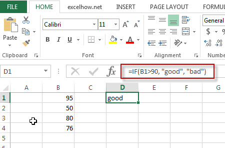
Note: the above excel formula will test a condition “b1>90”, if the condition is true, then “good” will return or “bad” will return.

Nested IF statements

The excel if function just only test one condition and if you want to deal with more than one condition and return different actions depending on the result of the tests,  then you need to include several IF statements (functions) in one excel IF formula, these multiple IF statements are also called Excel Nested IF formula(Nested IFs).

For example:

=IF(A1>=80, "excellent", IF(A1>=60, "good", IF(A1>0, "bad", "no valid score")))

More reading: Excel Nexted IF Functions (Statements) Tutorial

Excel Logical operators

When you are writing an If statement, you may need to use any of the following excel logical operators:

Operator	Meaning	Example	Description
=	Equal To	A1=B1	Returns True if a value in cell A1 is equal to the values in cell B1; FALSE if they are not.
>	Greater Than	A1>B1	Returns True if a value in cell A1 is greater than the values in cell B1; FALSE if they are not.
>=	Greater Than or Equal to	A1>=B1	Returns True if a value in cell A1 is greater than or equal to the values in cell B1; FALSE if they are not.
<	Less Than	A1<B1	Returns True if a value in cell A1 is less than the values in cell B1; FALSE if they are not.
<=	Less Than or Equal to	A1<=B1	Returns True if a value in cell A1 is less than or equal to the values in cell B1; FALSE if they are not.
<>	Not Equal to	A1<>B1	Returns True if a value in cell A1 is not equal to the values in cell B1; FALSE if they are not.

Let’s see some examples for logical operators in Excel formula:

 =(A1>B1)
Output: TRUE

=(A1<B1)
Output: FALSE

=(A1>=B1)
Output: TRUE

=(A1<>8)
Output: FALSE

=(A1<>B1)
Output: TRUE

=(IF A1>3, “TRUE”, “FALSE”)
Output: TRUE

Frequently Asked Questions

Question1: I want to write an IF Formula based on the below test criteria in the Microsoft excel.

If the number in Cell B1 is greater than 30, then I want it to return A

If the number in cell B1 is between 20 and 30, then I want it to return B

If the number in Cell B1 is below 20, then I want it to return C

The below formula is what I currently write:

=IF(B1>30,"A",IF(B1<30,B1>20,"B","C"))

When I entered the above formula in the Cell C1, and it will return an Error.

Answer:  You can use IF function in combination with AND function to reflect the above logic. So you can do it using the following formula:

=IF(B1>30,"A",IF(AND(B1>=20,B1<=30),"B","C"))

Or you can use another IF formula without AND function as follows:

=IF(B1>30,"A",IF(B1<20,"C","B"))

Question 2: I want to write a excel Formula for sales rep, If the sales are less than 10K, then the member will get no commission. If the sales are between 10 and 50K, then the member will get a 3% commission. If the sales are more than 50k, then the member will get 5% commission. Could you help me?

Answer: Based on the above description, we can use the following excel IF formula:

=IF(B1<10,0,IF(B1<50,B1*3%,B1*5%))

Question 3: I want to select students for the scholarship in school, and based on the student’s scores and attendance value, if the student scores more than 85 and has the attendance of more than 85%, then he/she will get the scholarship. Please help me how to write this formula based on my test criteria.

Answer: you can use the IF function with the AND function to check whether both of two conditions are met or not. If the test are met, then return “Yes”, otherwise returns “No”.

So you can use the following IF formula in Excel:

=IF(AND(B1>85, C1>85%),"Yes","No")

Question 4:  I am trying to write an excel formula based on the following logic:

I want to enter a formula in Cell C1 that will Add B1, B2 and B3 or multiply B1 by 1, multiply B2 by 2, multiply B2 by 3, which action will be taken based on what you put in Cell D1.

Appreciated for any help. Thanks

Answer: Based on the above logic description, you need to use SUM function to count the sum of B1, B2 and B3. We can use the following IF formula:

=IF(D1="Add”,SUM(B1,B2,B3),IF(D1="Multiply",B1*B2*B3,"ERROR"))

Question 5:  I am trying to write a formula in excel to check the employee number field and returns the relevant band of employee. I already have one IF formula, but I always return the first value of “A”. Could you help?

=IF(B1>=10,"A",IF(B1>=20,"B",IF(B1>=50,"C")))

Answer:  when you write an IF nested formula, you need to start with the largest number first or start the smallest number first with less than or equal to operator.

1# start with the largest number first, we can write down the below formula:

=IF(B1>=50,"C",IF(B1>=20,"B",IF(B1>=10,"A")))

2# start with the smallest number first, you need to change the >= to <= , just see the below formula:

=IF(B1<=10,"A",IF(B1<=20,"B",IF(B1<=50,"C")))

Question 6: I want to write a Formula in excel to return “bad” if the cell B1 is either <100 or >500, otherwise, it should be returned the value of cell B1.

Answer: For the above logic test, we should use the OR function in the IF condition, so we can write down the below IF formula:

=IF(OR(B1>500,B1<100),"good",B1)

Question 7: I want to write a formula in excel using IF function to check if the cell B1 >10 and B1<20. If TRUE, returns “good”, If FALSE, returns “bad”

Answer: You can use IF function in combination with AND function to check the value of Cell B1, if cell B1 is greater than 10 and cell B1 is less than 20, then returns “good”, otherwise, it will return “bad”.

=IF(AND(B1>10,B1<20),"good","bad")

Question 8:  I need to write a nested IF statement in excel 2013 to check the following logic:

If Cell B1 is less than 5, then multiply it by 5.

If Cell B1 is greater than or equal to 5 but less than 10, then multiply it by 10.

If cell B1 is greater than 10, then multiply it by 15.

Answer: This is a generic nested IF formula in excel, we can write the below nested IF statement to reflect the logic.

=IF(B1<5, B1*5, IF(B1<10, B1*10, B1*15))

Question 9:  I want to write a formula to match the following logic in MS Excel 2013:

If A1*B1 <=10, then returns A

If A1*B1 >10 but A1*B1 <=20, then returns B

If A1*B1 >20 but A1*B1 <=30, then returns C

If A1*B1>30, then returns D

Answer: You can use IF function to build a Nested IF statement in combination with AND function to achieve it. Let’s write down the following IF formula:

=IF(A1*B1<=10,"A", IF(AND(A1*B1>10,A1*B1<=20),"B", IF(AND(A1*B1>20,a1*B1<=30,"C","D"))))

Question 10: I want to write an IF function to check if the value in cell B1 is blank or Text string or Numeric value, if the cell B1 is empty, then return “blank”, if the cell B1 is a text string, then return “Text”, if the value in cell B1 is a numeric value, then return “number”. Any help for this formula, thanks.

Answer: Based on the description, you need to use ISBLANK function to check if the value in cell b1 is blank or not. And need to use ISTEXT function to check if the value in cell B1 is a text string or not and need to use ISNUMBER function to check if the value in cell B1 is a number or not. So you can write a nested IF statements in combination with ISBLANK, ISTEXT and ISNUMBER functions in Excel as follows:

=IF(ISBLANK(B1),"blank", IF(ISTEXT(B1),"Text", IF(ISNUMBER(B1),"number")))

Question 11:  I want to write a formula in excel to calculate the bonus for employees in company, if the employee salary is greater than or equal to $2000, then the bonus will be 10% of the salary , otherwise, the bonus will be 5% of the employee salary.

Answer:  we need to check if the salary in Cell B1 (it’s the salary of the first employee) is greater than or equal to 2000. It the condition test is TRUE, then returns B1*10%, otherwise returns b1*5%. So we can write down the following IF formula in excel:

=IF(B1>=2000, B1*10%, B1*5%)

Question 12: In Microsoft Excel 2013, I want to create an IF function to check if any employee who have at least 10 years of experience and whose salary is greater than $5000, If TRUE, then the bonus will be 20% of salary.

Answer: you can use IF function in combination with AND function to check if the value in cell B1 is greater than or equal to 10 and the value in Cell C1 is greater than 5000. If both of two conditions are TRUE, then returns C1*20%, otherwise returns “No Bonus”.

Let’s write down the following IF statement as follows:

=IF(AND(B1>=10,C1>5000),C1*20%, "No Bonus")

Question 13: I want to create an IF formula in Excel 2013 to check the following text logic:

If B1<10, then multiply B1 by 1%, but the returned value is not less than 50.

If B1>10, then multiply B1 by 2%, but the returned value is not greater than 100.

Answer: To reflect the first test condition, you need to use MAX function to match the condition. To reflect the second test condition, you need to use MIN function to match that the returned value should not be greater than 100. So we can use the following excel IF formula:

=IF(B1<10, MAX(50,B1*1%), IF(B1>10, MIN(100,B1*5%)))

Question 14:  I want to use IF function to check if B1 is greater than 10 and B2 is greater than 20 and B3 is less than 30, if TRUE, then returns “good”, otherwise, it should be returned “bad”.  So How to create the IF formula based on the above test criteria to check three conditions at the same time.

Answer: you need to use AND function within the IF function in excel to create an IF formula as follows:

=IF(AND(B1>10,B2>20,B3<30),"good","bad")

Question 15:  I have an IF formula that might cause a division by zero error, I don’t know how to avoid this kind of errors in Excel formula.

Answer: You can use ISERROR function to catch this kind of errors then use the IF function to check the returned values from ISERROR function to avoid an error. So we can write an IF function in combination with ISERROR function in excel. For example, we can use the following IF formula:

=IF(ISERROR(B1/C1),0, B1/C1)

The ISERROR function will return TRUE when trying to divide B1 by 0.

Question 16:  I need to create a formula in Excel 2013 to reflect the following logic:

If B1=Excel, then return E

If B1=word, then return W

If B1=access, then return A

Answer:  You can use IF function to create a nested IF statements as follows:

=IF(B1="Excel","E",IF(B1="word","W",IF(B1="access","A")))

Question 17:  I have a worksheet that containing cells that are formatted as date format. I want to write an IF formula to check the first value in Cell (month part). So I am trying to create the following IF formula:

=IF(LEFT(B1,1)=8, "August","Null")

The returned results are always “Null”.

Answer: As the dates are not recognized as string, so you cannot use the LEFT function to exact the first value in the dates. At this moment, you need to use Month function to convert the date to its month number in Excel. So we can write down the below IF formula in combination with Month function:

=IF(MONTH(B1)=8, "August","Null")

Question18: I am trying to create an IF formula to check if the time value in cells are greater than 10.00h for the following date format: 08/11/2018 09:43.50.  Appreciative of any help.

Answer: In excel, you can use HOUR, MINUTE, SECOND functions to compare the date or time value. so if you want to compare the value in Cell B1 if it is greater than 10h, then you can use HOUR function within IF function, just like this: HOUR(B1)>10, so we can write down the below formula:

=IF(HOUR(B1)>10, "greater","less")

Question 19: I want to create an IF function and need to combine with another RAND function.  The formula just works find for the first IF_VALUE_TRUE statement, but the formula works not good for IF_VALUE_FALSE statement. Here is the IF formula I have got:

=IF(ISBLANK(B1),"","=rand()")

In the above IF function, it will return empty string when the value in cell B1 is blank. Otherwise, it should add a random function, the problem is that the cell doesn’t run the RAND function. So how can I fix it?  Thanks

Answer:  when you write an IF formula, if you want to enclose others function, you need not to add quotes around the RAND () function, so just remove the quotes and equal sign in your IF function. Just like the below IF formula:

=IF(ISBLANK(B1),"",RAND())

Question 20: I am trying to write an IF formula in Excel 2013 to reflect the following logic:

If B1 is greater than or equal to 50 and C1 is 0

OR

If B1 is greater than or equal to 30 and C1 is greater than or equal to 1

OR

If B1 is greater than or equal to 20 and C1 is 2

Then take the following action:  D2/E2

Otherwise, return FALSE

I have wrote the following IF formula, but it doesn’t work at all.

=IF(AND(B1>=50,C1>=0),OR(AND(B1>=30,C1>=1)),OR(AND(B1>=20,C1>=2)),D2/E2,"FALSE")

Answer: you need to nest your different AND function within an OR function in the IF formula. So you can try the below IF formula:

=IF(OR(AND(B1>=50,C1>=0),AND(B1>=30,C1>=1),AND(B1>=20,C1>=2)), D2/E2,"FALSE")

Question 21: I want to create an IF function in combination with MID function in excel 2013. it need to check if the value in one specified cell is TRUE, then return the first six characters from another cell. Otherwise return empty value.

Answer: you just need to add MID function within IF function in excel, and do not add any quotes around MID function.    So you can use the following IF formula to achieve your request:

=IF(B1=TRUE, MID(C1,1,5), "")

Question 22:  I have a excel worksheet as below:

A     B

——

20   O

30   V

10   T

50   T

I want to create an IF formula to reflect the following logic:

IF cell A1 is less than or equal to 30 and Cell B1 is equal to “O” or “V”, if TRUE, then returns 300, otherwise returns 400.

IF Cell A1 is greater than 30 and Cell B1 is equal to “O” or “V”, then returns 500, otherwise returns 600.

I have wrote the below tow IF formulas for the above two conditions as follows:

=IF(AND(A1<=30,OR(B1="O",B1="V")),300,400)

=IF(AND(A1>30,OR(B1="O",B1="V")),500,600)

I am able to check the above two IF formula and the returned results is OK… But I am not able to combine the above two IF formula into a single IF formula. So anybody can help? Many thanks

Answer:  Based on the above logic, you can use the below IF formula to combine with above two IF formulas:

=IF(A1<=30,IF(OR(B1="O",B1="V"),300,400),IF(OR(B1="O",B1="V"),500,600))

Question 23: I am trying to write an IF function to prevent zero and negative values in cells. What I would like is that if the value in cell B1 is less than or equal to 0, then it should be returned “Null” otherwise, it should return the calculation of Cells value, like as:B2*(C2-D2)*E2.

The below IF formula is what I have:

=IF(B1<=0,"Null","B2*(C2-D2)*E2")

When I run the formula above, it only returns my calculation string and do not take the actual calculation.

Answer: In excel, the double quotes make any values in between be recognized as Text string. So if you want to take calculation for your IF formula, just remove the double quotes.  Let’s see the modified IF formula as follows:

=IF(B1<=0,"Null",B2*(C2-D2)*E2)

Question 24: I want to create an new IF function to check if the value in cells is Saturday or Sunday, If TRUE, returns “yes”, otherwise, returns “No”. And I am using the following IF formula, but I get an error, so what’s wrong for this formula?

=IF((OR($B1="Saturday","$B1="Sunday"),"yes","no"))

Answer: you need to use the WEEKDAY function within IF function to handle the dates if they are in date format, like as: 11/8/2018.

So you can use the below IF function to achieve your logic:

=IF(WEEKDAY($B$1,2)>5,"yes","no")

You can also use TEXT function within the IF function to achieve the same results, just like the below IF formula:

=IF(LEFT(TEXT($B$1,"ddd"))="S","yes","no")

Question 25: I want to write an IF function in excel to check if the first character in one Cell is equal to 5, then the returned value should be the five rightmost characters of that cell, otherwise, the returned value should be the four rightmost characters. I wrote one IF formula as follows, but it doesn’t work.

=IF(LEFT(B1,1)=5, RIGHT(B1,5),RIGHT(B1,4))

In the above IF function, it always return the rightmost four characters even though the first character in Cell B1 starts with “S”.  Please help me to fix it.

Answer: you should know the returned value of the LEFT function firstly in excel. As the LEFT function will return a Text value, so you also need to provide a string for comparison, so adding quotes to enclose it. Just like the below IF function:

=IF(LEFT(B1,1)="5", RIGHT(B1,5),RIGHT(B1,4))

There is another way to achieve the same results, you can use NUMBERVALUE function to convert the result of LEFT function to a numeric value, like the below IF function:

=IF(NUMBERVALUE(LEFT(B1,1))=5,RIGHT(B1,5),RIGHT(B1,4))

Question 26:  I have 2 columns contain date and time or just only contain time. And I want to check if the times of column A is greater than the times of column B. the key issue may be that column A has the date and time.  I wrote the following IF formula to run it in Cell C1, but it returned the inaccurate results.

=IF(A1>B1,"yes","no")

Any help would be appreciated… Many thanks!

Answer:  the date part of the value in column A is the integer, while the time is the decimal. You can use the following IF formula:

=IF(A1-INT(A1)>B2),"yes","no")

Question 27:  The below are the results that I expected, and I want cell B1 to B4 can detect the string from A1 to A4 automatically and return the same string value plus the severity level when the test match. For example, If A1 is equal to “critical”, then it should be returned “critical severity 1” in the cell B1. Etc.

And I am using the following IF formula, but it does not work at all. Please help to fix it. Thanks

=IF(A1="Critical","Critical Severity 1",""),IF(A1="High","High Severity 2",""),IF(A1="Medium","Medium Severity 3",""),IF(A1="Low","Low Severity 4","")

A	B
critical	critical severity 1
high	high severity 2
medium	Medium severity 3
low	low severity 4

Answer: you can try to run the following IF formula in excel:

=IF(A1="critical","critical Severity 1",IF(A1="high","high Severity 2",IF(A1="medium","medium Severity 3",IF(A1="low","low Severity 4",""))))

Question 28: I am working on an excel file and want to create a new IF formula to reflect the following logic:

If the value in Cell A1 is equal to the value in Cell A2, then check if the minus of B1 and B2 is equal to a special value, and if the condition is TRUE, returns “yes”, otherwise, returns “no”.  Here is the IF formula I have:

=if(A1=A2,B1-B2=5 or B1-B2=-5 or B1-B2=20 or B1-B2=-20, "yes", "no")

Any help is appreciated…Thanks

Answer: you need to use OR function with IF function to create a nested IF statement to achieve your request. So you can try the following Excel IF formula in your excel file.

=IF(A1=A2,IF(OR(B1-B2=5,B1-B2=-5,B1-B2=20,B1-B2=-20),"yes","no"),"no")

Question 29: I want to create an IF formula to check the range of cells in excel.  I have scores of different subject for a student, and want to check if any one of scores is less than 60, If TRUE, then return “BAD”.  Can this logic be done with the IF statements in excel 2013?

Answer: you can use COUNTIF function within IF function to create a generic IF formula as follows:

=IF(COUNTIF(B:B,"<60")>0,"BAD","Good")

Question 30: I am trying to create a new IF statement so that when the formula is looking at Row A and Row B, the returned values should be shown in the Row C. the following logic need to be checked:

IF the value in the Row A is equal to “NA” And the value in the Row B is equal to “NA”, then return “NA” value in Row C.

IF the value in the Row A is equal to “NA”, and the value in the Row B is equal to “denied”, then return “denied” value in Row C.

IF the value in the Row A is equal to “allowed” and the value in the Row B is equal to “NA”, then return “allowed” value in Row C.

Here is my formula:

=IF(AND(A1 = "NA", B1 = "NA"),"NA",IF(OR(A1="denied",B1 ="denied"),"denied", "NA"))

I don’t know how to include “allowed” in the IF formula above, anyone can help this, many thanks.

Answer: This is a typical nested if statement, you can use OR function within IF function in excel. We can write down this nested IF formula as follows:

=IF(OR(A1="denied", B1="denied"), "denied", IF(OR(A1="allowed", B1="allowed"), "allowed", "NA"))

• Excel AND function
  The Excel AND function returns TRUE if all of arguments are TRUE, and it returns FALSE if any of arguments are FALSE.The syntax of the AND function is as below:= AND (condition1,[condition2],…) …
• Excel ISBLANK function
  The Excel ISBLANK function returns TRUE if the value is blank or null.The syntax of the ISBLANK function is as below:= ISBLANK (value)…
• Excel COUNTIF function
  The Excel COUNTIF function will count the number of cells in a range that meet a given criteria.= COUNTIF (range, criteria) …
• Excel ISERROR function
  The Excel ISERROR function returns TRUE if the value is any error value except #N/A. The ISERROR function is a build-in function in Microsoft Excel and it is categorized as an Information Function. The syntax of the ISERROR function is as below: = ISERROR (value) …
• Excel LEFT function
  The Excel LEFT function returns a substring (a specified number of the characters) from a text string, starting from the leftmost character.The syntax of the LEFT function is as below:= LEFT(text,[num_chars])…
• Excel MID function
  The Excel MID function returns a substring from a text string at the position that you specify. The MID function is a build-in function in Microsoft Excel and it is categorized as a Text Function. The syntax of the MID function is as below: = MID (text, start_num, num_chars) …
• Excel TEXT function
  The Excel TEXT function converts a numeric value into text string with a specified format. The syntax of the TEXT function is as below:= TEXT (value, Format code)…
• Excel RIGHT function
  The Excel RIGHT function returns a substring (a specified number of the characters) from a text string, starting from the rightmost character…

More Excel IF Formula Examples

---

• Excel nested if function
  The nested IF function is formed by multiple if statements within one Excel if function. This excel nested if statement makes it possible for a single formula to take multiple actions…
• Excel IF formula with Equal to logical operators
  The “Equal to” logical operator can be used to compare the below data types, such as: text string, numbers, dates, Booleans.  This section will guide you how to use equal to logical operator in excel IF formula with text string value and dates value…
• Excel IF formula with greater than logical operators
  How to use if function with greater than, greater than or equal to,  less than and less than or equal to logical operators in excel. Let’s see the below generic if formula with greater than operator: =IF(A1>10,”excelhow.net”,”google”) …
• Excel IF formula with AND logical function
  You can use the IF function combining with AND function to construct a condition statement. If the test is FALSE, then take another action. The syntax of AND function in excel is as follow: =AND(condition1,[condition2],…)…
• Excel IF function with OR logical function
  If you want to check if one of several conditions is met in your excel workbook, if the test is TRUE, then you can take certain action. You can use the IF function combining with OR function to construct a condition statement…
• Excel IF function with “NOT” logical function
  If you want to check several test conditions in an excel formula, then take different actions. You can use NOT function in combination with the AND or OR logical function in excel IF function…
• Excel IF formula with AND & OR logical functions
  If you want to test the result of cells based on several sets of multiple test conditions, you can use the IF function with the AND and OR functions at a time…
• Excel IF Function With Numbers
  If you want to check if a cell values is between two values or checking for the range of numbers or multiple values in cells, at this time, we need to use AND or OR logical function in combination with the logical operator and IF function…
• Excel IF function with text values
  If you want to write an IF formula for text values in combining with the below two logical operators in excel, such as: “equal to” or “not equal to”…
• Excel IF function with Dates 
  If you have a list of dates and then want to compare to these dates with a specified date to check if those dates is greater than or less than that specified date. …
• Excel IF function check if the cell is blank or not-blank
  If you want to check the value in one cell if it is blank or empty cell, then you can use IF function in combination with ISBLANK function or logical operator (equal to) in excel…

• Excel nested if statements with ranges
  Many people usually asked that how to write an excel nested if statements based on multiple ranges of cells to return different values in a cell? How to nested if statement using date ranges? How to use nested if statement between different values in excel 2013 or 2016…

• Count Cells That Contain Specific Text
  This post will discuss that how to count the number of cells that contain specific text or certain text in a specified cells of range in Excel. How to get the total number of cells that contain certain text.……
• Sum Values by Group
  Assuming that you have a table that contain the product name and its sales result. And you have group by those values based on the product name, then you want to sum values based one each product name. You can create a new Excel formula based on the IF function and SUMIF function.…
• Get nth Largest Value with Duplicates
  If you want to get the largest unique value in a data set with duplicates, you can create a new excel array formula based on the MAX function and the IF function..…
• Find the Largest Value Based on Multiple Criteria
  Assuming that you have a list of data that you want to find the largest value based on the product “excel” and the sales region “east”. You can create a new excel formula based on the SUMPRODUCT function and the LARGE function..……
• Create a Five Star Rating System
  How do I change the five points system to five star rating in excel. How to use the conditional formatting function to create a five star rating system in excel…..
•  Rank values in a column based a specific value in another column
  Assuming that you have a list of data contains two columns and the first column is product list and another is Sales number. You want to rank the sales number of a specified product name. You can try to write a complex formula based on the IF function and the COUNTIFS function to achieve the result..…
• Comparing Columns Using Conditional Formatting Icon Sets
  how to compare the adjacent cells in the different columns using Conditional Formatting Icon Sets in Excel.  How to compare Columns or rows using Conditional Formatting Icon Sets to show increase or decrease status in your current worksheet..…
• Show Only Positive Values
  You can create a formula based on the IF function, and the SUM function to sum all values in the range A1:C5 and just show only positive values…
• Count Unique Values Using Pivot Table
  You can insert a 3rd or helper column with a formula to check if the value is unique in the selected range of cells, and the create pivot table based on the 1st and 3rd column to count unique values..…
• Compare Dates
  Assuming that you have a list of data that contain date values in Excel, you can use the IF function to create a formula to achieve it. If the date is greater that the given date value, then return True. Otherwise, it returns False….
• Excel Vlookup Return True or False
  you can use the VLOOKUP function to look for a value in a column in a table and then returns TRUE from a given column in that table if it finds something. If it doesn’t, it returns FALSE …
• VLOOKUP Return Multiple Values Horizontally
  You can create a complex array formula based on the INDEX function, the SMALL function, the IF function, the ROW function and the COLUMN function to vlookup a value and then return multiple corresponding values horizontally in Excel.…
• Copy and Paste Only Non-blank Cells
  If you want only copy non-blank cells in a range in Excel, you need to select the non-blank cells firstly, then press Ctrl +C keys to copy the selected cells. So how to only select all non-blank cells in the selected range in your worksheet..…
• Changing Negative Number to Zero in Excel
  If you want to change all negative numbers to zero value from a cell in Excel, you can use a formula based on the MAX function or IF function.…
• Count Dates in Given Year/Month/Day in Excel
  You can create a formula based on the SUMPRODUCT function and the YEAR function to count dates by a give year….
• Generate All Possible Combinations of Two Lists
  You can use a formula based on the IF function, the ROW function, the COUNTA function, The INDEX function and the MOD function to get a list of all possible combinations from those two list….
• Find Missing Numbers in a Sequence in Excel
  You can use an excel array formula based on the SMALL function, the IF function, the ISNA function, the MATCH function, and the ROW function to find missing numbers in a sequence…

The logical IF statement in Excel is used for the recording of certain conditions. It compares the number and / or text, function, etc. of the formula when the values correspond to the set parameters, and then there is one record, when do not respond — another.

Logic functions — it is a very simple and effective tool that is often used in practice. Let us consider it in details by examples.



The syntax of the function «IF» with one condition

The operation syntax in Excel is the structure of the functions necessary for its operation data.

=IF(boolean;value_if_TRUE;value_if_FALSE)

Let us consider the function syntax:

• Boolean – what the operator checks (text or numeric data cell).
• Value_if_TRUE – what will appear in the cell when the text or numbers correspond to a predetermined condition (true).
• Value_if_FALSE – what appears in the box when the text or the number does not meet the predetermined condition (false).

Example:

Logical IF functions.

The operator checks the A1 cell and compares it to 20. This is a «Boolean». When the contents of the column is more than 20, there is a true legend «greater 20». In the other case it’s «less or equal 20».

Attention! The words in the formula need to be quoted. For Excel to understand that you want to display text values.

Here is one more example. To gain admission to the exam, a group of students must successfully pass a test. The results are listed in a table with columns: a list of students, a credit, an exam.

The statement IF should check not the digital data type but the text. Therefore, we prescribed in the formula В2= «done» We take the quotes for the program to recognize the text correctly.



The function IF in Excel with multiple conditions

Usually one condition for the logic function is not enough. If you need to consider several options for decision-making, spread operators’ IF into each other. Thus, we get several functions IF in Excel.

The syntax is as follows:

Here the operator checks the two parameters. If the first condition is true, the formula returns the first argument is the truth. False — the operator checks the second condition.

Examples of a few conditions of the function IF in Excel:

It’s a table for the analysis of the progress. The student received 5 points:

• А – excellent;
• В – above average or superior work;
• C – satisfactory;
• D – a passing grade;
• E – completely unsatisfactory.

IF statement checks two conditions: the equality of value in the cells.

In this example, we have added a third condition, which implies the presence of another report card and «twos». The principle of the operator is the same.

Enhanced functionality with the help of the operators «AND» and «OR»

When you need to check out a few of the true conditions you use the function И. The point is: IF A = 1 AND A = 2 THEN meaning в ELSE meaning с.

OR function checks the condition 1 or condition 2. As soon as at least one condition is true, the result is true. The point is: IF A = 1 OR A = 2 THEN value B ELSE value C.

Functions AND & OR can check up to 30 conditions.

An example of using the operator AND:

It’s the example of using the logical operator OR.

How to compare data in two tables

Users often need to compare the two spreadsheets in an Excel to match. Examples of the «life»: compare the prices of goods in different bringing, to compare balances (accounting reports) in a few months, the progress of pupils (students) of different classes, in different quarters, etc.

To compare the two tables in Excel, you can use the COUNTIFS statement. Consider the order of application functions.

For example, consider the two tables with the specifications of various food processors. We planned allocation of color differences. This problem in Excel solves the conditional formatting.

Baseline data (tables, which will work with):

Select the first table. Conditional Formatting — create a rule — use a formula to determine the formatted cells:

In the formula bar write: = COUNTIFS (comparable range; first cell of first table)=0. Comparing range is in the second table.

To drive the formula into the range, just select it first cell and the last. «= 0» means the search for the exact command (not approximate) values.

Choose the format and establish what changes in the cell formula in compliance. It’s better to do a color fill.

Select the second table. Conditional Formatting — create a rule — use the formula. Use the same operator (COUNTIFS). For the second table formula:

Download all examples in Excel

Now it is easy to compare the characteristics of the data in the table.

The syntax of the IF() function is the following:

= IF ( logical_test , [value_if_TRUE] , [value_if_FALSE] )

The first two attributes are obligatory, i.e. without them, the formula doesn’t work, and produces an error message.

• logical _test – a placeholder for the condition we want to test
• value_if_TRUE – an attribute where we need to specify a value (text, or another function) that the IF formula returns when the result of the logical_test is TRUE

The third parameter is Optional, i.e. we can skip it and in such a case, the IF() function returns the default value FALSE.

• value_if_FALSE – an attribute for a value, text or another formula that the IF() function must return when the result of the logical test is FALSE.

In other words, IF() function is used to test the specific conditions and can be described as the statement:

IF something is true, THEN return the first value, ELSE – return then second value.

The simplest IF() function may be written with the first two parameters only.

For example, this formula is absolutely correct:

 =IF(C2=1,"Hello!")

This formula tests the condition we set (C2=1) and if it is true, the formula returns the text message (“Hello!”).

Otherwise, it returns the default value FALSE.

Interesting Fact!!! You can use another simpler test in Excel for a certain condition. Just place a formula like “=C2>C3” in a cell and press ENTER. If this statement is true, the formula returns the default value – TRUE. Else (i.e. when a value in C2 is NOT larger than a value in C3 cell) the formula will return another default value – FALSE. We use the IF() function in these cases; when we want to trigger some further actions or calculations depending on the results of the logical test.

Typically, the IF() function is used in situations when we need to calculate or flag the results based on certain conditions (for example, smaller than, equal to, greater than and others).

Despite the fact that Excel usually provides multiple choices on how to solve every specific task, the IF() function can play a good role in such cases.

Another simple example of the IF() function:

=IF(C3="Hello!",1, 0)

If a value of the C3 cell is the text “Hello!” then this formula returns the one (1) value.

Else (i.e. if this cell contains any other text, number or blank value), the formula returns zero.

The big advantage of the IF() function (like many other Excel functions) is how we can replace all three arguments in this example with whatever we want/need and it still works properly (if we follow the syntax, of course).

For example, let’s replace the one (as a value_if_true) to another formula “C3+C4” and replace zero value (0) to TODAY() function.

Our initial formula becomes:

=IF(C3="Hello!",C2+C3,TODAY())

That means – IF a value in C2 cell equals one, THEN do the addition C2+C3.

ELSE (i.e. when C2 doesn’t equal “Hello!”), THEN execute the TODAY() function and return its result.

IF() function is a universal function, i.e. it accepts as an attribute different types of a value, such as numeric value, text, date/time, other functions, named ranges and others).

The IF function can be easily used as a part of other more complex formulas.

Moreover, you can use the so-called nested IF() function and replace the [value_if_false] with another IF() function.

The most common reason to do that is when you need to create a multi-choice comparison like a waterfall.

The last value_if_FALSE attribute is a value that we want the formula to return if the result of ALL logical tests in the formula is FALSE.

We know that we need to use a nested IF() (i.e. one IF() inside another IF() statement) when we have a “but” keyword inside the sentence with a logical test.

Take a look at the screenshot below.

In this example, we need to add the text “flag” if a value is greater than 200, BUT if this value is less than 50 we need to return “follow up” text.

We know that we need to use a nested IF() when there is the “but” keyword in the logical test.

Pro Tip: Be cautious. The more IF iterations we use, the more complex the formula becomes and the more difficult it is to understand. In addition, the complex formulas that contain multiple IF functions along with other Excel functions may slow down the calculation speed, especially if they use large ranges of cells. Also, it’s very easy to make an accidental mistake or typo inside the long and complex formulas, and such errors are difficult to trace properly.

The IF() function is often used with other logical functions such as AND() or OR() functions that we will discuss further.

Let’s look at some practical examples…

TEST CASE №1 Adding the word “Good” if the Revenue is greater than 15000

This is a typical use of the IF() function.

Let’s flag all apps if their Revenue is above 15,000.

Step 1. Go to the first cell where we need to insert a formula (cell C5 in this example).

Start the formula with an equal sign (=), add the keyword IF and the opened parentheses to make the formula look like:

=IF(

Step 2. The first argument of the IF() function is a logical test.

In this example, we want to flag a value in cell B5 (Revenue) if it is above 15000.

So, let’s continue the formula =IF(B5>15000,

Do not forget to put a comma once this step is ready.

This coma is used by Excel as a delimiter to separate the arguments from each other.

Pro tip: We can either type a numeric value in the logical test or use a cell reference to a cell that contains such a value (C2 cell in our example). The second approach is preferred because it gives us more flexibility in the future. Once we copy/paste the formula to the entire range, all we need to do in this case – if want to change that value – is go to the referral cell and change it there without needing to re-write the formula for all related cells.

NOTE: Keep in mind that if we want to use this approach, we need to fix the cell reference to look like $C$2. This fixed cell address is required for copying the formula to the entire range. Without that, the formula will return the wrong result. We can simply press F4 to fix the cell reference in the formula (make sure that the cursor is located near the appropriate cell address)

The formula becomes:

=IF(B5>$C$2,

Step 3. The second argument of IF() function, as we remember, is a value_if_TRUE.

Let’s type the text “Good” as a second attribute in the formula:

=IF(B5>$C$2, "Good",

Do not forget to put a comma once this step is ready.

Also, be careful – if you type a text value, you need to put it inside a double quotation mark (“your text”)

Pro tip: We can either type a numeric value in the logical test or use a cell reference to a cell that contains such a value (C3 cell in our example). If in the future we’ll decide to change the “Good” word to something else (“Not Bad”, for example), then all we need to do is go to cell C3 and change that text in the cell without the necessity to re-do the entire formula.

Our formula becomes:

=IF(B5>$C$2,$C$3,

NOTE: Don’t forget to fix the cell reference to look like $C$3 address. Press F4 to make an absolute reference. Without that, the formula will return a wrong result.

Step 4. The third argument of the IF() function is value_if_FALSE. We can skip this attribute (in such cases Excel returns the default value – FALSE). However, if we want to do that in a more aesthetic way, let the formula return a blank value. The blank value in Excel is equal to nothing between two quotation marks, like “”. So, the final version of the formula becomes:

=IF(B5>$C$2,$C$3,"")

NOTE: Don’t forget to close the brackets and press ENTER.

Step 5. Drag the formula down to the entire range.

Make a quick check manually to ensure that the formula returns the correct result according to our expectations.

TEST CASE №2 Adding the word “Good” if the Revenue is greater than 15000 and less than 20000

Let’s flag all apps if their Revenue is above 15,000 but under 20,000

Step 1. Go to the first cell where we need to insert a formula (cell D5 in this example).

Start the formula with an equal sign (=), add the keyword IF and the opened parentheses to make the formula look like:

=IF(

Step 2. The first argument of the IF() function is a logical test.

In this example, we want to flag a value in cell B5 (Revenue) if it is above 15000 and less than 20,000.

This is a typical situation when we can use the AND() logical function to unite several certain conditions into a single logical test.

AND() function can accept up to 255 conditions as its arguments.

Let’s continue the formula and add the second keyword AND with an opened parenthesis.

Once we’ve done that, we can type both conditions for the logical test inside AND() block and close its second parenthesis.

The formula looks like:

=IF(AND(B5>$D$2,B5<$D$3),

NOTE: Don’t forget to fix the cell reference to look like $D$2 and $D$3 address.

Press F4 to make an absolute reference.

Without that, the formula will return a wrong result after we drag it down to the entire range.

NOTE: Don’t forget to use a comma once this step is ready.

This comma is used by Excel as a delimiter to separate the arguments from each other.

Step 2. The second argument of IF() function, as we remember, is a value_if_TRUE.

Let’s add another cell reference as a second attribute in the formula:

=IF(AND(B5>$D$2,B5<$D$3),$C$3,

NOTE: Don’t forget to put a comma after the attribute once this step is ready. Be careful. If you type a text value, you need to put it inside a double quotation mark (“your text”)

Step 3. The third argument of the IF() function is a value_if_FALSE.

We can skip this attribute and Excel returns the default value – FALSE.

However, the more aesthetic way to do that is to return nothing (or blank value).

Nothing in Excel is denoted as a double quotation mark without any space:

=IF(AND(B5>$D$2,B5<$D$3),$C$3,"")

NOTE: Don’t forget to close the bracket and press ENTER.

Step 4. Drag the formula down to the entire range.

Make a quick check manually to ensure that the formula returns the correct result according to our expectations.

TEST CASE №3 Adding the word “Good” if the Revenue is greater than 15000 and less than 20000. Adding the word “Exceptional” if the Revenue is greater than or equal to 20,000. Otherwise, keeping the values

This time we’ll flag all apps as “Good” if their Revenue is above 15,000 and under 20,000.

In addition, we’ll flag them as “Exceptional” if their Revenue is greater than or equal to 20,000

Step 1. Go to the first cell where we need to insert a formula (cell E5 in this example).

Start the formula with an equal sign (=), add the keyword IF and the open parentheses to make the formula look like:

=IF(

Step 2. The first argument of the IF() function is a logical test.

The first part of the formula in this example is the same as we wrote in the previous example:

=IF(AND(B5>$E$2,B5<$E$3),$C$3,

NOTE: Don’t forget to to put a comma after the attribute once this step is ready.

Step 3. Usually, the third argument of the IF() function is a value_if_FALSE.

However, this time we need to add the second condition when a value in cell B5 is greater than or equal to 20,000.

We can do that if we use nested IF() function.

Let’s add another IF() block as a third parameter now:

=IF(AND(B5>$E$2,B5<$E$3),$C$3,IF(

Step 4. Add the second logical test, and the second value_if_TRUE.

In our example, the formula must return the “Exceptional” keyword if the value in cell B5 is greater than or equal to 20,000.

Let’s type this:

=IF(AND(B5>$E$2,B5<$E$3),$C$3,IF(B5>=$E$3,"Exceptional",

NOTE: If you type a value as a text, you need to put it inside a double quotation mark (“your text”)

Step 5. We need to write a value that the formula will return if the result of both logical tests is FALSE.

In our example, the formula must return the raw Revenue value in this case.

Let’s place this attribute as the third argument in the second IF() block:

=IF(AND(B5>$E$2,B5<$E$3),$C$3,IF(B5>=$E$3,"Exceptional",B5))

NOTE: Don’t forget to close the brackets.

We created two IF blocks, so we need to close two brackets at the end.

Step 6. Drag the formula down to the entire range.

Make a quick check manually to ensure that the formula returns the correct result according to our expectations.

TEST CASE №4 Adding the word “Flag” if the Revenue is greater than or equal to 20,000 OR it is lesser than or equal to 15,000

Let’s flag all apps if their Revenue is <= 15,000 or >= 20,000

Step 1. Go to the first cell where we need to insert a formula (cell D5 in this example).

Start the formula with an equal sign (=), add the keyword IF and the open parentheses to make the formula look like:

=IF(

Step 2. The first argument of the IF() function is a logical test.

In this example we want to flag a value in cell B5 (Revenue) if it is below or equal to 15000 OR above or equal to 20,000.

This is a situation when we can use OR() logical function that allows the testing of multiple logical conditions and return a true value if ANY of them is true.

Let’s continue the formula and add the second keyword OR with an opened bracket.

Once we’ve done that, we can type both conditions for the logical test inside OR() block and close its second parentheses.

The formula looks like:

=IF(OR(B5>=$F$2,B5=<$F$3),

NOTE: Press the F4 button on the keyboard to make an absolute reference.

Step 3. The second argument of the IF() function, as we remember, is a value_if_TRUE.

Let’s add this attribute in the formula:

=IF(AND(B5>$D$2,B5<$D$3),"Flag",

NOTE: If you type a text value, you need to put it inside a double quotation mark (“your text”)

Step 4. The third argument of the IF() function is a value_if_FALSE.

Let’s add a double quotation mark without any space to return a blank value:

=IF(AND(B5>$D$2, B5<$D$3),"Flag","")

NOTE: Don’t forget to close the bracket and press ENTER.

Step 5. Drag the formula down to the entire range.

Quickly check to ensure that the formula returns the correct result.

TEST CASE №5 Using other formulas inside the logical functions

Let’s calculate the difference between Actual Revenue and Budget Revenue and flag those cases when the difference is larger than +/- 10%.

Step 1. The easiest way to start building such a complex formula is to calculate the core value (this is the +/-10% threshold value in our case).

Step 2. Go to the first cell where we need to insert a formula (cell D23 in this example).

Start the formula with an equal sign (=), add the formula to calculate the difference (Actual divided by Budget minus one:

=B23/C23 - 1

Step 3. Let’s add the IF() block and the appropriate logical test.

This is a situation when we can use the OR() logical function as we need to flag a value if it is greater than +10% or lower than -10%:

=IF(OR(B23/C23 - 1>10%,B23/C23 - 1<-10%),

Step 4. The second argument of the IF() function, as we remember, is a value_if_TRUE.

In this example we need to return the exact deviation, so let’s do that, by simply copying the initial formula.

=IF(OR(B23/C23 - 1>10%,B23/C23 - 1<-10%),B23/C23 - 1,

Step 5. The third argument of the IF() function is a value_if_FALSE.

Let’s add a double quotation mark without any space to return a blank value:

=IF(OR(B23/C23 - 1>10%,B23/C23 - 1<-10%),B23/C23 - 1,"")

NOTE: Don’t forget to close the bracket and press ENTER.

Step 6. Drag the formula down to the entire range.

Quickly check to ensure that the formula returns the correct result.

TEST CASE №6 Using text symbols as the result of the IF() function

Let’s mark the positive deviation with the up arrow and the negative deviation with the down arrow.

Step 1. We’ll continue the previous example.

Let’s say we want to mark all positive deviations with a symbol that looks like an up arrow and all negative deviations with a symbol that looks like a down arrow.

First of all, a few preparations.

Let’s go to the cells above the test range (A20 and A21 cells in this example).

Feel free to select any other cells if you prefer.

Step 2. Insert the symbols that will indicate all positive and negative deviations.

To do this, we need to go on the INSERT tab on the Excel Ribbon and follow the path: INSERT > Symbol > Arial > Geometric Shapes

Click Insert once you have selected a shape.

Go to another cell below and insert the second arrow in the same way.

Step 3. Go to the first cell in the range where we want to add these visual indicators.

Replicate the IF() function with the cell references containing the arrows as the value_if_TRUE and value_if_FALSE attributes.

=IF(B23/C23 - 1>10%,$A$20,IF(B23/C23 - 1<-10%,$A$21,""))

NOTE: Don’t forget to close the bracket and press ENTER.

Step 4. Drag the formula down to the entire range.

Quickly check that the formula returns the correct result.

Workbook for Download

Feel free to Download the Workbook HERE.