
You can use a simpler version of this complicated function by creatively using the Median formula:
In our first example above, the range is 20-60, upon checking the value 50, it is in between this range.
The median formula will return the value in the middle of these 3 values when arranged in increasing order: 20, 50, 60. The median value is 50.
Since it matches the value we are evaluating, then the answer we get is a Yes, this value (50) is in between the range.
Now that you have learned how to use Excel if between two numbers, let’s move forward to dates and text.
Irrespective of how you format a cell to display a date, Excel always stores it as a number. The number stored for each date actually represents the number of days since 0-Jan-1990.
1st Jan 1990 is stored as 1 (representing 1 day since 0-Jan-1990) and 23rd June 2020 is stored as 44,005 (representing 44005 days since 0-Jan-1990).
So, to check whether a date is in between two mentioned dates, we have the same application as the median formula.
Below is an example of how to use the median function to check dates.
In our first example above, the range is May 1 – July 1, upon checking the date June 1, it is in between this range.
The median formula will return the value in the middle of these 3 dates when arranged in increasing order: May 1, June 1, July 1. The median value is June 1.
Since it matches the value we are evaluating, then the answer we get is a Yes, this value (June 1) is in between the range.
For text, we are checking if the value is alphabetically in the middle. We will be using the and formula:
Conclusion
In this tutorial, you have learned how to use Between formula in Excel even when there is no explicit formula available to do this. You can use a combination of various other available function to create Excel if between range functionality.
You can use MIN, MAX, MEDIAN & AND functions to create a creative Between function in Excel for numbers, dates and text.
HELPFUL RESOURCE:
Make sure to download our FREE PDF on the 333 Excel keyboard Shortcuts here:

HELPFUL RESOURCES:
Get access to 30+ Microsoft Excel & Office courses for ONLY $1.
Источник
Excel IF statement between two numbers or dates
 by Alexander Frolov, updated on March 7, 2023
The tutorial shows how to use an Excel IF formula to see if a given number or date falls between two values.
To check if a given value is between two numeric values, you can use the AND function with two logical tests. To return your own values when both expressions evaluate to TRUE, nest AND inside the IF function. Detailed examples follow below.
Excel formula: if between two numbers
To test if a given number is between two numbers that you specify, use the AND function with two logical tests:
- Use the greater then (>) operator to check if the value is higher than a smaller number.
- Use the less than ( smaller_number, value =) and less than or equal to ( = smaller_number, value =AND(A2>10, A2
To check if A2 is between 10 and 20, including the threshold values, the formula in C2 takes this form:
In both cases, the result is the Boolean value TRUE if the tested number is between 10 and 20, FALSE if it is not:

If between two numbers then
In case you want to return a custom value if a number is between two values, then place the AND formula in the logical test of the IF function.
For example, to return «Yes» if the number in A2 is between 10 and 20, «No» otherwise, use one of these IF statements:
If between 10 and 20:
If between 10 and 20, including the boundaries:

Tip. Instead of hardcoding the threshold values in the formula, you can input them in individual cells, and refer to those cells like shown in the below example.
Suppose you have a set of values in column A and wish to know which of the values fall between the numbers in columns B and C in the same row. Assuming a smaller number is always in column B and a larger number is in column C, the task can be accomplished with this formula:
Including the boundaries:

And here is a variation of the If between statement that returns a value itself if TRUE, some text or an empty string if FALSE:
Including the boundaries:

If boundary values are in different columns
When smaller and larger numbers you are comparing against may appear in different columns (i.e. number 1 is not always smaller than number 2), use a slightly more complex version of the formula.
=AND(A2>=MIN(B2, C2), A2
To return your own values instead of TRUE and FALSE, use the following Excel IF statement between two numbers:
=IF(AND(A2>MIN(B2, C2), A2
=IF(AND(A2>=MIN(B2, C2), A2

Excel formula: if between two dates
The If between dates formula in Excel is essentially the same as If between numbers.
To check whether a given date is within a certain range, the generic formula is:

In case, the start and end dates are in predefined cells, the formula becomes much simpler:
Where $E$2 is the start date and $E$3 is the end date. Please notice the use of absolute references to lock the cell addresses, so the formula won’t break when copied to the below cells.

Tip. If each tested date should fall in its own range, and the boundary dates may be interchanged, then use the MIN and MAX functions to determine a smaller and larger date as explained in If boundary values are in different columns.
If date is within next N days
To test if a date is within the next n days of today’s date, use the TODAY function to determine the start and end dates. Inside the AND statement, the first logical test checks if the target date is greater than today’s date, while the second logical test checks if it is less than or equal to the current date plus n days:

If date is within last N days
To test if a given date is within the last n days of today’s date, you again use IF together with the AND and TODAY functions. The first logical test of AND checks if a tested date is greater than or equal to today’s date minus n days, and the second logical test checks if the date is less than today:

Hopefully, our examples have helped you understand how to use the If between formula in Excel efficiently. I thank you for reading and hope to see you on our blog next week!
Practice workbook
You may also be interested in
Table of contents
Hello!
Hope you can help me out — how to calculate how many B values in a repeating range A values with a range of 1 row.
For example: A B C B D A C B B D A A C B B D . here there are 3 ranges of A values and I need your help how to know how many B values in each interval.
Thank you so much!
Reply
Hi!
I don’t really understand in which ranges do you want to count characters. But I hope this guide will be helpful to you: How to count characters in Excel cell and range. If that’s not enough, explain the problem in more detail.
Hello, I wish to create an IF function that will provide me with variable results based on dates occurring before a date input directly into the formula. So, if C8, D8 and E8 are all less than 1/1/24, it give me one result, but if only 1 or 2 are before, I get different results based on how many dates are before the input date in the formula.
I am currently trying to get the following formula to work:
Hello!
To input the correct date in a formula, use DATE function. Read more in this manual: Excel DATE function with formula examples to calculate dates.
How do I place a formula to give 150 as result if gross salary is between kshs 0-6000, and formula to give 300 as result if gross salary is between ksh 6001- 8000, and the formula to give 400 as result if gross salary is between kshs 8001- 12000.
Hi!
You can find the answer to your question in this article: Nested IF in Excel – formula with multiple conditions
I need a formula to give me a fixed percentage based on two figures. Looking at the retirement fund lump sum withdrawal benefits tax income table (how much will the member be taxed on) I want to build a formula that once I put the person’s fund value in one cell it will show me the percentage taxable in another cell.
Table is as follow:
Between 1 — 27 500 = 0%
Between 27 501 — 726 000 = 18%
Between 726 001 — 1 089 000 = 27%
Between 1 089 001 and above = 36%
Hi!
Please check out the following article on our blog, it’ll be sure to help you with your task: Excel nested IF statement — multiple conditions in a single formula.
Firstly, thanks for the great content. It’s helped me a lot (but I’m stuck!)
I’m trying to compare 2 numbered lists.
In List A, I have a list of numbers ranging from 6-11 digits in length, where each cell (A2, An) is a unique number.
In List B, I have a different format, where column E & F are called Low Range & High Range respectively. It’s purpose is to create a range where the number is sequential and doesn’t break, if it breaks, it moves to the next range.
For Example:
The following numbers are depicted differently in both Lists below (200000, 200001, 200002, 200004, 200006, 200007, 200008, 200010)
List A:
Cell A2 = 200000
Cell A3 = 200001
Cell A4 = 200002
Cell A5 = 200004
Cell A6 = 200006
Cell A7 = 200007
Cell A8 = 200008
Cell A9 = 200010
List B:
Cell E2 (Low Range) = 200000 — Cell F2 (High Range) = 200002 (i.e. includes 200001)
Cell E3 (Low Range) = 200004 — Cell F3 (High Range) = 200004
Cell E4 (Low Range) = 200006 — Cell F4 (High Range) = 200008 (i.e. includes 200007)
Cell E5 (Low Range) = 200009 — Cell F5 (High Range) = 200009
Problem I’m trying to solve:
I’m trying to compare each cell (A2, An) in List A to each Low Range & High Range (Column E & F) combination. I have it working when I specify an individual cell in List A (A2) and compare it to E2 & F2 in List B using the following formula:
Hello!
If I understand your task correctly, the following formula should work for you:
You Sir are a genius! Many thanks Alexander!
Trying to get a formulae to work which will populate a cell.
If A2 is between 1-6 then in H2 will show Low, if A2 is between 7-12 then in H2 will show Medium, if A2 is between 13-16 then in H2 will show High,
Cell A2 is a formulae arrived from other cells
tried the If statements but don’t appear to work
Condition
From- 1-Jan-23 (to) 10-Jan-23
within A,B,C & D, i have to mention «YES» if «A» contains dates fulfilling the above condition or «No» . likewise for B,C & D. Kindly help.
A 5-Jan-23 to 10-Feb-23
B 11-Jan-23 to 10-Feb-23
C 1-Jan-23 to 7-Jan-23
D 11-Jan-23 to 10-Feb-23
Hello!
If I understand correctly, each date interval is written as text in a cell. You can’t do any calculations with text. You can apply the recommendations described in the article above only if each date is written in a separate cell. To split the text into separate cells, I recommend using this instruction: Split string by delimiter or pattern, separate text and numbers. Then convert the text to date as described in the article at the link.
Hello, I’m trying to create a spreadsheet which returns overdue, active and imminent using the following formula. How can I express that when the date is 6 it returns OVERDUE. At the moment the imminent command is cancelling out the dates which should return ACTIVE.
sorry, that didn’t make sense.
I want it to display IMMINENT when TODAY is 6 from the date in H3.
oh boy, I’m sorry, the formula keeps changing when I post .
I want it to display IMMINENT when TODAY is greater than 4 but less than 6 compared with the date in H3.
Hi!
Based on your description, it is hard to completely understand your task. However, I’ll try to guess and offer you the following formula:
Hi!
I’m sorry, I’m afraid these pieces of info are not enough to give you a formula. Describe in detail the criteria for each of the three options and I will try to help
Thank You Alexander,
What I’m trying to create is a list of duties which need to be completed every 7 days.
In the H column, I want members of my team to type in the date that they last did the duty.
If the date inputted is more than 7 days from TODAY, I want the column with the formula in to to display «OVERDUE»
If the date is less than 7 but more than 2 days from TODAY, I what it to display «ACTIVE»
If the date is 2 days before TODAY, I want it to display IMMINENT
I have inherited the formula below but it never displays «IMMINENT». I am trying to amend this formula so that 2 days before it says OVERDUE, It flags up that the duty is imminent.
Sorry, I hadn’t seen your 2.16 reply. I’m not sure my 2.30 message made sense. I’ve just trying the formula you suggested.
Hi!
Try this formula
I am trying to add comment Late or On time based on 2 dates: I have a column for due date and a column for actual date
If due date and actual date are the same or actual date is earlier — then its on time
If actual date is later than due date its late.
How would I build this please?
Hi!
Compare two dates using the IF function:
=IF(A1>=B1, «On time», «Late»)
I want to input in a cell:
if value in N3 is between 0 and 7, then «7 days», if between 0 and 14, then «14 days», if between 0 and 30, then «30 days», if between 0 and 60, then «60 days»
I would appreciate your help
Hi!
Pay attention to the first paragraph of the article above. It covers your case completely.
I’m trying to create myself a time sheet — if I work less than 8 hours, i get a 30 min lunch break and if i work more than 8 hours i get a 45 min lunch break. So I’ve played around with a lot of different ways to do this, what i think isnt working is trying to get it to return a value in minutes. This is where I’ve got (but this doesnt work):
=IFS(D2=timevalue»8:00″,timevalue»00:45″)
Hi!
Use the TIME function to get a specific time value.
i have an urgent column with yes or no, and a date column. I want to create a due date by adding either 2 days if yes and 7 days if no.
Hi!
For multiple conditions, you can use the IFS function
I want to have a formula of startdate-31/12/22 but if startdate if lower than 01/01/22 then it will be just 12
Hello, i have struggle to find a formula for this » if up to 70% then 80%,if between 50%-70% then 50% and if between 40%-50% then 40%. I need this all in one row.
Thank you
Hi!
The answer to your question can be found in this article: Nested IF in Excel – formula with multiple conditions.
I am struggling to have multiple formula to create a target date for task completion.
Column A has revision numbers of the document ranging from 0 to 4
Column B has start date
Column C should be target date (if Column A contains 0, the Column C should be +14 days, — formula is =IF(C4=1,WORKDAY.INTL(NB,7,16)). I would like to repeat the same formula with different C column values for at least 4 times.
Hi!
Your formula does not match your question. I’m sorry, I’m afraid these pieces of info are not enough to give you a formula. Describe in detail what problem you have, and I will try to help you.
I need to calculate commissions based on % of MSRP by product line.
The % off of MSRP can vary between these cutoff amounts. Ie, the % MSRP could be 94% or 73%, the amounts don’t always fall along these specific cutoff values but at these cutoff values, the commission rate changes:
Column on worksheet % of MSRP % of MSRP % of MSRP
Product Line = 100% >= 92.50% >= 75%
column S 9% 6% 3%
column T 9% 6% 3%
column U 1% 1% 1%
column V 4% 2% 1%
MSRP is in column AD
I need assistance with the formula to calculate the commission if a sale falls between these cutoffs.
Hi!
If I understand the problem correctly, you can find the necessary instructions in the article above, as well as in this guide: Excel Nested IF statement.
hi if you can pls help
A B C D E F G
Week # Week # Vendor Amount Date
Wed 12/8/2021 1 1 11/30/2021
Wed 12/22/2021 2 1 11/30/2021
Wed 1/5/2022 3 2 12/13/2021
Wed 1/19/2022 4 2 12/16/2021
Wed 2/2/2022 5 2 12/20/2021
Wed 2/16/2022 6 3 12/23/2021
Wed 3/2/2022 7 3 12/25/2021
column «A» has a list of dates Column «B» has a list of the week number now when I enter a date in Column «G» column «D» should find the correct «week #» from column «B»
Hi!
You can use the VLOOKUP formula to find the week number from a list of dates.
I also recommend paying attention to the WEEKNUM function to get the week number.
thank you for the quick reply
the week number i have in column «B» is not the standard week number
the date i have in column «G» is not in Column «A» since the date in column «G» is a date between 2 rows in column «A»
any other sugetions?
abe
Hi!
I am not sure I fully understand what you mean.
I am trying to display a text value if a number between 198.4 and 350.5 is displayed, but the formula is not working for me, I am entering this formula:
Hi!
Please read the above article carefully.
Instead of AND(C5>MIN199,C5 199,C5 Reply
Hello,
I swear I’ve done this before but can’t for the life of me recall. I have two tables:
Table 1: Column C = a number I enter, Column D = a corresponding text based on table 2
Table 2: Column A = a lower limit, Column B = an upper limit, Column C = text
What I’m looking to do is IF Table 1, C = 10, so it is >= Table 2 Column A and Reply
In essence, you build a formula as explained in the «If between two numbers then» example, but instead of the hardcoded values, supply the corresponding references.
Assuming your table 2 is on Sheet2 beginning in row 2, use the following formula for D2 in table 1:
I’m currently building a number sequence, using 5 columns and 50 rows. The numbers can’t >9 if so they should +1 to the next row.
for example you enter 51410 in the respective 5 columns and underneath it then starts counting up from 51410 to 51411 etc.
I have been using the IF(AND function however eventually this sequence counts up from 9 going over the maximum value of 9.
A2 = 8 A3 =9
B2 = IF(AND(F63>=9,E63>=9),»0″,E63+1)
B3 = IF(F63=9,»0″,SUM(F63,1))
is there any way around this.
Hi!
Sorry, I do not fully understand the task. I don’t see a relation between your question and the example. Write an example of the data you want to get. Try this instruction to create a sequence of numbers: SEQUENCE function in Excel — auto generate number series.
I would like to calculate how many instances of a word based on the date range formula — example below using November 2022 as range:
Column C contains dates
Column F contains word: high, medium or low
Date range I am happy with & returns a value: =COUNTIFS($C:$C,»>=01/11/2022″,$C:$C,» Reply
Hello!
Add one more condition to the COUNTIFS formula.
How can I do a nested If statement with one of the the look up variables is a #. I have tried using wild cards, but end up with the same results.
=IF((Z2-Y2)0,»Late», IF(OR(COUNTIF(Z2, «*»&»#»&»*»)), «not received «, «»)))
The z2 and Y2 are date fields. The result is the same for the # it says #value!
Hello!
The answer to your question can be found in this article: COUNTIF formulas with wildcard characters (partial match). I hope my advice will help you solve your task.
here is my dilemma, if this can be done in excel or not.
I created a poker tracker sheet in excel to track my winnings on freerolls I play in, on various poker sites.
Now,
in Column D is my buy in, column E is won bounty and column H is price I won, and in column J is client name.
Now, how can I calculate in column K for each separate site and track my winnings from each separate site in column K??
Is it possible??
I.e. IF client name is GG then total winnings are.
IF client name is PS then total winnings are.
I wish I could post a screenshot to explain better what I mean.
Hello!
To calculate a sum based on one or more criteria, use the SUMIFS function. Look for the example formulas here: Excel SUMIFS and SUMIF with multiple criteria – formula examples. This should solve your task.
Copyright © 2003 – 2023 Office Data Apps sp. z o.o. All rights reserved.
Microsoft and the Office logos are trademarks or registered trademarks of Microsoft Corporation. Google Chrome is a trademark of Google LLC.
Источник
This article outlines how to use the IF with AND functions in Excel
How to Combine IF with AND functions
In Excel, you can combine IF with AND functions[1] to return a value based on two different numbers. It can be very useful when performing financial modeling and when you are creating conditional situations. In this article, learn how to build an IF statement between two numbers so you can easily answer the problem you’re trying to solve.
For example, if you are looking for a formula that will go into cell B2 and, if the number is between 100 and 999, then the result will be 100. Otherwise, if it is outside that range, then the result will be zero.
Download the Free Excel Template – IF with AND Functions.
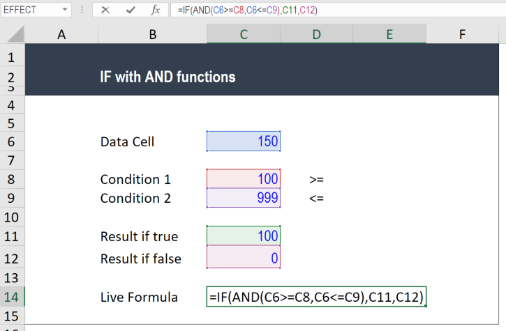
IF statement between two numbers
=IF(AND(C6>=C8,C6<=C9),C11,C12)
(See screenshots below).
Example of how to use the formula:
Step 1: Put the number you want to test in cell C6 (150).
Step 2: Put the criteria in cells C8 and C9 (100 and 999).
Step 3: Put the results if true or false in cells C11 and C12 (100 and 0).
Step 4: Type the formula =IF(AND(C6>=C8,C6<=C9),C11,C12).
Final result
Here is a screenshot in Excel after using the formula for an IF statement between two numbers. You can clearly see how the result from the example is 100 because the number 150 is between 100 and 999.
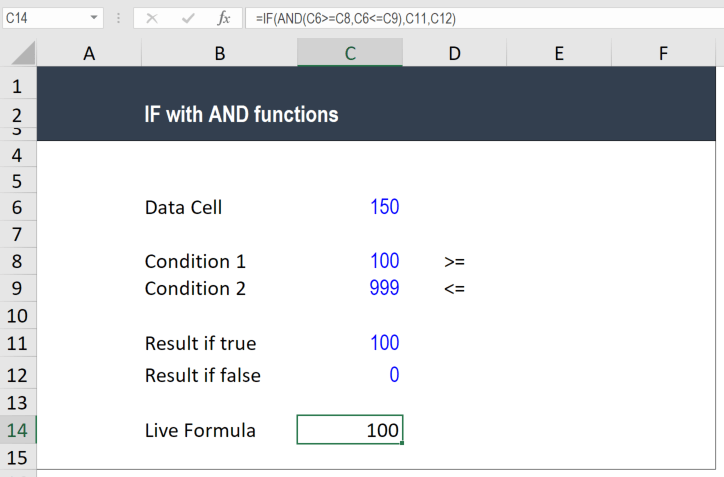
Congratulations, you have now combined IF with AND between two numbers in Excel!
Download the free template.
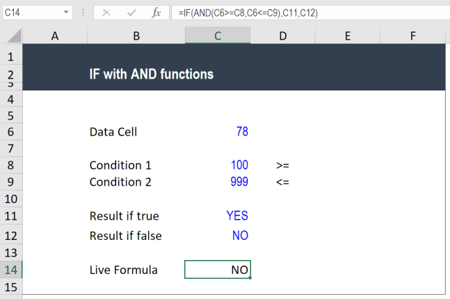
IF statement between two numbers (with text)
You don’t have to limit the resulting output from the model to only numbers. You can also use text, as shown in the example below. This time, instead of producing 100 or 0 as the result, Excel can display YES or NO to show if the argument is true or false.
More Excel Tutorials
Thank you for reading this guide to understanding how to use the IF function with the AND function in Excel to know if a number is between two other numbers. To keep learning and developing your career as a financial analyst, these additional CFI resources will help you on your way:
- Index and Match Functions
- Excel Shortcuts List
- Important Excel Formulas
- Advanced Excel Course
- See all Excel resources
The IF function allows you to make a logical comparison between a value and what you expect by testing for a condition and returning a result if that condition is True or False.
-
=IF(Something is True, then do something, otherwise do something else)
But what if you need to test multiple conditions, where let’s say all conditions need to be True or False (AND), or only one condition needs to be True or False (OR), or if you want to check if a condition does NOT meet your criteria? All 3 functions can be used on their own, but it’s much more common to see them paired with IF functions.
Use the IF function along with AND, OR and NOT to perform multiple evaluations if conditions are True or False.
Syntax
-
IF(AND()) — IF(AND(logical1, [logical2], …), value_if_true, [value_if_false]))
-
IF(OR()) — IF(OR(logical1, [logical2], …), value_if_true, [value_if_false]))
-
IF(NOT()) — IF(NOT(logical1), value_if_true, [value_if_false]))
|
Argument name |
Description |
|
|
logical_test (required) |
The condition you want to test. |
|
|
value_if_true (required) |
The value that you want returned if the result of logical_test is TRUE. |
|
|
value_if_false (optional) |
The value that you want returned if the result of logical_test is FALSE. |
|
Here are overviews of how to structure AND, OR and NOT functions individually. When you combine each one of them with an IF statement, they read like this:
-
AND – =IF(AND(Something is True, Something else is True), Value if True, Value if False)
-
OR – =IF(OR(Something is True, Something else is True), Value if True, Value if False)
-
NOT – =IF(NOT(Something is True), Value if True, Value if False)
Examples
Following are examples of some common nested IF(AND()), IF(OR()) and IF(NOT()) statements. The AND and OR functions can support up to 255 individual conditions, but it’s not good practice to use more than a few because complex, nested formulas can get very difficult to build, test and maintain. The NOT function only takes one condition.

Here are the formulas spelled out according to their logic:
|
Formula |
Description |
|---|---|
|
=IF(AND(A2>0,B2<100),TRUE, FALSE) |
IF A2 (25) is greater than 0, AND B2 (75) is less than 100, then return TRUE, otherwise return FALSE. In this case both conditions are true, so TRUE is returned. |
|
=IF(AND(A3=»Red»,B3=»Green»),TRUE,FALSE) |
If A3 (“Blue”) = “Red”, AND B3 (“Green”) equals “Green” then return TRUE, otherwise return FALSE. In this case only the first condition is true, so FALSE is returned. |
|
=IF(OR(A4>0,B4<50),TRUE, FALSE) |
IF A4 (25) is greater than 0, OR B4 (75) is less than 50, then return TRUE, otherwise return FALSE. In this case, only the first condition is TRUE, but since OR only requires one argument to be true the formula returns TRUE. |
|
=IF(OR(A5=»Red»,B5=»Green»),TRUE,FALSE) |
IF A5 (“Blue”) equals “Red”, OR B5 (“Green”) equals “Green” then return TRUE, otherwise return FALSE. In this case, the second argument is True, so the formula returns TRUE. |
|
=IF(NOT(A6>50),TRUE,FALSE) |
IF A6 (25) is NOT greater than 50, then return TRUE, otherwise return FALSE. In this case 25 is not greater than 50, so the formula returns TRUE. |
|
=IF(NOT(A7=»Red»),TRUE,FALSE) |
IF A7 (“Blue”) is NOT equal to “Red”, then return TRUE, otherwise return FALSE. |
Note that all of the examples have a closing parenthesis after their respective conditions are entered. The remaining True/False arguments are then left as part of the outer IF statement. You can also substitute Text or Numeric values for the TRUE/FALSE values to be returned in the examples.
Here are some examples of using AND, OR and NOT to evaluate dates.

Here are the formulas spelled out according to their logic:
|
Formula |
Description |
|---|---|
|
=IF(A2>B2,TRUE,FALSE) |
IF A2 is greater than B2, return TRUE, otherwise return FALSE. 03/12/14 is greater than 01/01/14, so the formula returns TRUE. |
|
=IF(AND(A3>B2,A3<C2),TRUE,FALSE) |
IF A3 is greater than B2 AND A3 is less than C2, return TRUE, otherwise return FALSE. In this case both arguments are true, so the formula returns TRUE. |
|
=IF(OR(A4>B2,A4<B2+60),TRUE,FALSE) |
IF A4 is greater than B2 OR A4 is less than B2 + 60, return TRUE, otherwise return FALSE. In this case the first argument is true, but the second is false. Since OR only needs one of the arguments to be true, the formula returns TRUE. If you use the Evaluate Formula Wizard from the Formula tab you’ll see how Excel evaluates the formula. |
|
=IF(NOT(A5>B2),TRUE,FALSE) |
IF A5 is not greater than B2, then return TRUE, otherwise return FALSE. In this case, A5 is greater than B2, so the formula returns FALSE. |

Using AND, OR and NOT with Conditional Formatting
You can also use AND, OR and NOT to set Conditional Formatting criteria with the formula option. When you do this you can omit the IF function and use AND, OR and NOT on their own.
From the Home tab, click Conditional Formatting > New Rule. Next, select the “Use a formula to determine which cells to format” option, enter your formula and apply the format of your choice.

Using the earlier Dates example, here is what the formulas would be.

|
Formula |
Description |
|---|---|
|
=A2>B2 |
If A2 is greater than B2, format the cell, otherwise do nothing. |
|
=AND(A3>B2,A3<C2) |
If A3 is greater than B2 AND A3 is less than C2, format the cell, otherwise do nothing. |
|
=OR(A4>B2,A4<B2+60) |
If A4 is greater than B2 OR A4 is less than B2 plus 60 (days), then format the cell, otherwise do nothing. |
|
=NOT(A5>B2) |
If A5 is NOT greater than B2, format the cell, otherwise do nothing. In this case A5 is greater than B2, so the result will return FALSE. If you were to change the formula to =NOT(B2>A5) it would return TRUE and the cell would be formatted. |
Note: A common error is to enter your formula into Conditional Formatting without the equals sign (=). If you do this you’ll see that the Conditional Formatting dialog will add the equals sign and quotes to the formula — =»OR(A4>B2,A4<B2+60)», so you’ll need to remove the quotes before the formula will respond properly.
Need more help?

See also
You can always ask an expert in the Excel Tech Community or get support in the Answers community.
Learn how to use nested functions in a formula
IF function
AND function
OR function
NOT function
Overview of formulas in Excel
How to avoid broken formulas
Detect errors in formulas
Keyboard shortcuts in Excel
Logical functions (reference)
Excel functions (alphabetical)
Excel functions (by category)
-
Excel Howtos
Between Formula in Excel [Quick Tips]
-
Last updated on June 24, 2010

Chandoo
In today’s quick tip, lets find how to check for between conditions in Excel using formulas, like this:

Between Formula in Excel for Numbers:
Lets say you have 3 values in A1, A2 and A3. And you want to find out if A1 falls between A2 and A3.
Now, the simplest formula for such a thing would be test whether the conditions A1>=A2, A1<=A3 are both true. Hence, it would look like,
=if(AND(A1>=A2,A1<=A3),"Yes", "No")
However, there are 2 problems with a formula like above:
1. It assumes that A2 is smaller than A3.
2. It is just too big.
Shouldn’t there be a shorter and simpler formula?!?
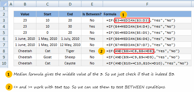
Well, there is. Last week when chatting with Daniel Ferry, he mentioned a darned clever use of MEDIAN formula to test this. It goes like,
=if(A1=MEDIAN(A1:A3),"Yes","No")
Now, not only does the above formula look elegant and simple, it also works whether A2 is smaller or larger than A3.
Between Formula in Excel for Dates:
Well, dates are just numbers in Excel. So you can safely use the technique above to test if a given date in A1 falls between the two dates in A2 and A3, like this:
=if(A1=MEDIAN(A1:A3),"Yes","No")
Between Formula for Text Values:
Lets say you want to find-out if the text in A1 is between text in A2 and A3 when arranged alphabetically, a la in dictionary. You can do so in Excel using,
…
wait for it…
…
that is right, <= and >= operators, like this:
=if(AND(A1>=A2,A1<=A3),"Yes", "No")
Between Formulas in Excel – Summary and Examples:
Here is a list of examples and the corresponding Excel Formulas to test the between condition.
Do you check for Between Conditions in Excel?
Checking if a value falls between 2 other values is fairly common when you are working with data. I would love to know how you test for such conditions in excel? What kind of formulas do you use?
Share using comments.
Recommended Excel Formula Tutorials:
- Check for Either Or conditions in Excel
- Find out if 2 ranges of dates overlap using formulas
- Get my Excel Formulas e-Book, learn 75 most used formulas overnight
Share this tip with your colleagues

Get FREE Excel + Power BI Tips
Simple, fun and useful emails, once per week.
Learn & be awesome.
-
208 Comments -
Ask a question or say something… -
Tagged under
and(), between formula, Excel 101, if() excel formula, Learn Excel, logical operators in excel, median() formula, Microsoft Excel Formulas, quick tip, spreadsheets, using excel
-
Category:
Excel Howtos

Welcome to Chandoo.org
Thank you so much for visiting. My aim is to make you awesome in Excel & Power BI. I do this by sharing videos, tips, examples and downloads on this website. There are more than 1,000 pages with all things Excel, Power BI, Dashboards & VBA here. Go ahead and spend few minutes to be AWESOME.
Read my story • FREE Excel tips book


Excel School made me great at work.
5/5

From simple to complex, there is a formula for every occasion. Check out the list now.

Calendars, invoices, trackers and much more. All free, fun and fantastic.

Power Query, Data model, DAX, Filters, Slicers, Conditional formats and beautiful charts. It’s all here.

Still on fence about Power BI? In this getting started guide, learn what is Power BI, how to get it and how to create your first report from scratch.
Related Tips
208 Responses to “Between Formula in Excel [Quick Tips]”
-
Clever use of MEDIAN, but it returns «Yes» if you use the upper or lower number. Whether you want to consider 20 as being «between» 10 and 20 is up to you.
Also, the examples made it harder to understand. In the first formula you use A1:A3 for the range, but the first picture looks like the formula is filled across rows, not columns.
-
@JP —
MEDIAN can be used regardless of your definition of «between.» To include the boundary points, I would write it like this:
.
=A1=MEDIAN(A1:A3)
.
To exclude them:
.
=A1=MEDIAN(A1,A2+1,A3-1)
.
Regards,
Daniel Ferry
excelhero.com-
 Lucky says:
 Hi I want to find out the difference in two numbers. But if the second number is minus it should not turn into plus in the results. Could you tell me the formula for it. Example (21.32)(-6.37) MY expectation to get the difference in between these two numbers. The answer should be 14.95. I do not hope the answer as 27.69. The actual mathematical answer that turn the second minus into plus and adds together. But excel always give me the second answer but please tell me the formula for the first answer. The deference between the numbers. Thanks
-
@Lucky
=21.32-abs(-6.37)
or
=Abs(A1)-Abs(A2)
-
-
-
Rob says:
Daniel —
your formula to exclude the boundary points would only work if you’re dealing strictly with integers. For example, if you test if 19.5 is between 10 and 20 using A1=MEDIAN(A1,A2+1,A3+1), it would fail.
Rob
-
Rob says:
I should clarify…I think it’s a very creative use of MEDIAN and if you’re testing numbers and want to include the end points, it’s a simpler method, but you need to use the other style using just instead of = to properly not include end points.
Rob -
Rob says:
darn…should have known my greater than and less than characters would be removed.
Meant to say you need to use the and() style test using just less than and greater than characters without the equal signs.
Rob -
cALi says:
I tried it using spanish MEDIANA(…) function, but it didn’t work. This is what I did, not such stylish, but it works fine: =IF(AND(A1=MIN(B1:C1)),»YES»,»NO»).
cALi
-
@Rob —
You bring up a good point that I should have clarified. When using the method I shared above to exclude the boundary points, the user is responsible for the precision. I have used this technique for years with operations scheduling and task management, often with a precision of days. However, I have used it with finer precision, hours, minutes, seconds. Again this is totally up to the user; he can use whatever value he wants instead of the integers of one:
.
=A1=MEDIAN(A1,A2+1/24,A3-1/24)
.
=A1=MEDIAN(A1,A2+1/24/60,A3-1/24/60)
.
=A1=MEDIAN(A1,A2+1/24/60/60,A3-1/24/60/60)
.
…of course those constants could/should be replaced by defined names.
.
Taking this to the extreme, one could easily define a constant that equals the smallest positive value that Excel can represent:
.
spv: =2.229E-308
.
We can then write the formula as:
.
=A1=MEDIAN(A1,A2+spv,A3-spv)
.
…which will work for any possible decimal value between the boundary points. It’s a robust and elegant solution, imo.Regards,
Daniel Ferry
excelhero.com -
cALi says:
Sorry, when copying and pasting, I should made some mistake, this is real one:
=IF(AND(A1=MIN(B1:C1)),»YES»,»NO»)A1: tested in Between Value
B1 and C1: limits -
cALi says:
I suppose HTML is in conflict with the code. Same code, different order of the arguments in the AND function:
=IF(AND(A1>=MIN(B1:C1),A1<=MAX(B1:C1)),»YES»,»NO») -
David says:
The formula =IF(A1=MEDIAN(B1:C1),»Yes»,»No») does not work when I tested it. It returns «No» for any value in A1, regardless if it falls between B1 and C1 or not.
-
@cALi —
I have no experience with the Spanish version of Excel, but I would be very surprised to learn that the worksheet functions differed in their outputs! Can you provide the exact formula (in Spanish) that did not work for you?
.
On a different note, here is an equivalent formula to yours, that does not use the AND() function, nor the IF() function:
.
=A1=MIN(MAX(A1:B1),MAX(B1:C1))
.
BTW, your formula (and hence my variation of it) has the characteristic where «between» includes the lower boundary point, but not the higher one. This can be altered in a similar fashion as my above example.
.
Regards,
Daniel Ferry
excelhero.com -
@Daniel —
We can also do both.For example, I created a data validation in cell H2 consisting of «True,False» values. (That is, True and False without quotes).
This formula would then allow you to toggle the output as exclusive or inclusive of the start and end numbers by changing the value in H2 (True means exclude, False means include):
=B3=MEDIAN(B3,C3+N(H2),D3-N(H2))
-
@JP —
That’s it!
Imagine the nested IF monster that you just avoided! Good job.
That is why I am always going on about better solutions to haplessly using IF(), when one understands the problem.
.
Regards,
Daniel Ferry
excelhero.com -
cALi says:
@Daniele
Thanks for your time, I made some mistake since testing both alternatives I received the same results:
=An=MIN(MAX(An:Bn),MAX(Bn:Cn))
=An=MEDIAN(An:Cn)Indeed, your solution is not just elegant but also practical, I could name it «minimalist».
Best regards,
cALi -
@David.. you have to include A1 as well to get it right. Like this,
=IF(A1=MEDIAN(A1,B1,C1),”Yes”,”No”)
-
sam says:
@ JP Instead of True/False use 1,0, we can then drop the N()
=B3=MEDIAN(B3,C3+H2,D3-H2)
-
Tim Buckingham says:
Turned into UDF for kicks
Function ISBETWEEN(Rng, num1, num2) As Boolean
‘ Checks if value between num1 and num2
Dim Low As Double, Hi As DoubleISBETWEEN = False
Low = Application.Min(num1, num2)
Hi = Application.Max(num1, num2)If Rng Is Nothing Then Exit Function
If Rng = Application.WorksheetFunction.Median(Rng, Low, Hi) Then ISBETWEEN = TrueEnd Function
I like how easy it is to read when wanting to count the values that fall between using
=COUNTIF(Rng,ISBETWEEN(Rng,Num1,Num2))
-
Gerald Higgins says:
I think the use of the MEDIAN function is very clever.
Nitpicking now.
If I understand correctly, Daniel’s suggestion for an amendment to exclude the =boundaries case as in
=A1=MEDIAN(A1,A2+1/24,A3-1/24)
assumes that all the numbers involved are positive.
If one or both of the boundary numbers are negative, I think this formula will produce wrong results for values of A1 just outside the true boundary range.Also, this formula
=A1=MIN(MAX(A1:B1),MAX(B1:C1))
works as long as the C1 value is higher than the B1 value, but not the other way round, which was described asa fault in the OP.
This formula solves that particular problem (it’s essentially the same as cALi’s)
=AND(A1MIN(B1:C1))
Replace < with <= as required. -
Gerald Higgins says:
Sorry, lost symbols in my last post.
I’ll try again.
The last formula should be
=AND(A1 (less than symbol) MAX(B1:C1),A1 (greater than symbol) MIN(B1:C1)) -
elad says:
CooL :)))) very elegant solution !
-
Guest says:
Great use of the function — I will be using this.
As always though, formulaic results are only as good as the data on which they’re based (it’s spelled «coyote» instead of «cayote,» so your last text example should actually read yes. 🙂
Not to nitpick….but to nitpick… 🙂 -
@sam —
«Instead of True/False use 1,0, we can then drop the N()»
That’s true, but who’s going to understand that? If your users can, they’re much smarter than mine.
-
[…] the problem is similar to between formula trick we discussed a few days back, yet very […]
-
[…] Between Formula in Excel, Chandoo presents some formulas for determining if a given value is in between two known […]
-
Daniel’s spv approach does not work because the spv addon never makes it into the mantissa of the floating point numbers.
Regards,
Bernd -
@Bernd —
With all due respect, you should double check that.
-
Daniel,
Excel 2010 (version 14.0.4760.1000 32 bit), spv set to 2.229E-308, A1 = 1, A2 = 1, A3 = 2, result A1=MEDIAN(A1,A2+spv,A3-spv) = True (should be False).
Again, if I am not mistaken, the very small value does not make it into the mantissa of the MEDIAN parameters which will then lead to MEDIAN(1,1,2) = True.
Regards,
Bernd -
Daniel,
I do like the spv idea. My suggestion to fix the mantissa issue would be something like this:
=A1=MEDIAN(A1,A2+POWER(10,INT(LOG10(A2))-14),A3-POWER(10,INT(LOG10(A3))-14))
But this is sort of a monster formula again. Maybe two functions InfInc and InfDec (for infinitesimal increase / decrease) should be introduced which return the smallest float greater than the input (resp. the greatest float which is smaller).
Regards,
Bernd -
@Bernd —
.
Touche.
.
While the formula logic is correct, Excel does not handle the very, very small number correctly in this instance. Good bug catch.
.
As I mentioned above, I have used the MEDIAN method countless times, but usually with dates, but also to the precision of hours, minutes, and seconds. I’ve never actually tried to use it with such fine precision before. I should have tested it before commenting, as Murphy’s Law always prevails.
.
After testing I discovered that 1E-14 is the finest precision where my idea does work. To be sure, this will work in virtually every situation, as this is a very small number:
.
0.00000000000001
.
In fact, this is exactly what your POWER/LOG formula results in. So there is no need to use the monster formula.
.
Instead of defining spv as the smallest possible value (in Excel) we can simply enter it’s definition as:
.
=1e-14
.
and now spv can stand for the smallest possible value (handled correctly). -
Daniel,
I am sorry, but — no, you cannot take an absolute 1e-14. Please note that my POWER/LOG formula flexibly adjust itself to the number in question:
For 1 it’s 1e-14, for 10 it’s 1e-13, for 100 it’s 1e-12, …
It will exactly impact on the lowest digit of the mantissa. Please note that it can be different for the two MEDIAN border parameters. Please see my example at
http://www.sulprobil.com/html/test_if_between_2_values.html
Regards,
Bernd -
Rick Rothstein (MVP — Excel) says:
There is always this purely mathematical method for determining if a value (A1) is between two limits (A2 and A3) excluding the end points…
=If(ABS(A1-((A2+A3)/2)).LT.ABS(A3-A2)/2,»Yes»,»No»)
To make it include the end points, change the less than to less than or equal….
=If(ABS(A1-((A2+A3)/2)).LE.ABS(A3-A2)/2,»Yes»,»No»)
Note that I used (with the surrounding dots) .LT. for the «less than» symbol and .LE. for the «less than or equal» symbol. Now, the only thing I am unsure of is how to adjust this for the spv that was brought up in the latter comments… anyone want to take a stab at it?
-
Rick,
Your ABS approach makes perfect sense for small numbers (ASCII code) or floats that are in the same ball park.
But test the values 0, 1, 2, 3, …, 9 on the border values 1e16 and 5 with .LT. and with .LE.
The ABS approach gets it horribly wrong here because the lower border value 5 gets off the mantissa when added or subtracted to or from 1e16.
Regards,
Bernd -
Rick Rothstein (MVP — Excel) says:
@Bernd,
While it is possible, of course, I would not normally expect a test for inclusion within a range to have such wildly divergent end points for the range.
-
Rick,
Why risk anything if you can only lose? If I deal with floating point numbers of unknown size and if I need to know whether a number is between two others I would use neither the MEDIAN approach nor the ABS approach.
I think it’s far more important to know the basics about floating point numbers than to know this MEDIAN «trick» or the ABS comparison:
http://docs.sun.com/source/806-3568/ncg_goldberg.html
Regards,
Bernd -
Debbie says:
Thanks for posting…! Worked perfectly for what I needed!!!
-
sanjeev khendi says:
i want to if function/ if total sales 200000 ,then com rate =5% give me information how to solve it with example
-
Hui… says:
@Sanjev
Assuming you are entering this in the cell representing Com Rate
=if(sum(sales range)>=200000,5%,10%)
10% is the value for Com Rate if sales -
cALi says:
@Sanjev
Using Daniel Ferry approach about IF function, which I have embraced as mine:C D E
Lower Limit Upper Limit Commission Rate
? -
cALi says:
@Sanjev
Using Daniel Ferry approach about IF function, which I have embraced as mine:C D E
Lower Limit Upper Limit Commission Rate
4 Range1 — 100,000.00 0%
5 Range2 100,000.00 200,000.00 2%
6 Range3 200,000.00 1,000,000.00 5%
7 Range4 1,000,000.00 1E+100 6%
8
9 Actual Sales 180,000.00
Comm. Rate 2% =SUMPRODUCT((C4:C7 -
cALi says:
@ Chandoo, really sorry for the mess, the text editor is definitely not my friend… this will be my last chance, I hope it works…
@ Sanjeev,
Using Daniel Ferry IF function approach, and using some dummy data:A B C D
Lower Limit Upper Limit Commission Rate
3 Range1 — 100,000.00 0%
4 Range2 100,000.00 200,000.00 2%
5 Range3 200,000.00 1,000,000.00 5%
6 Range4 1,000,000.00 1E+100 6%
7 Actual Sales 180,000.00
8 Comm. Rate 2% =SUMPRODUCT((B3:B6?$B$7)*($B$7?C3:C6)*D3:D6)Please replace ‘?’ with ‘less than or equal to’ and ‘?’ with ‘less than’ proper operators.
By the way, C6 is a dummy value, is ‘upper infinite’ to make this approach work.Regards,
cALi -
[…] Between Formula in Excel […]
-
KM says:
Sales Achievement
15,001 — 20,000 EL
20,001 — 50,000 E
50,001 — 100,000 D
100,001 — 160,000 C
160,001 — 240,000 B
240,001 & above AIf the sales achievement fall in between 50,001-100,000 is under Class D, can you help if i have many column of acheivement data which fall under different class. How can i set the formula in one time?
-
@KM
Are your Ranges in 1 Column or 3
ie: is 15,001 – 20,000 in 1 cell or 3 cells -
I want drop my serial no continuous automatically from the input value
e.g I have list of TV I given code for that
TV001
TV002
TV003
THEN I START ADDING BIKE
BIKE001
BIKE002
AGAIN I WANT ADD TV FROM PREVIOUS NUMBER CONTINUATION
LIKE
TV004
TV005
again i want add bike003 cotinuation from last number
IS THERE ANY FORMULAS FOR THAT?
PLEASE SEND THIS TO MY EMAIL ADDRESS sent to mani.n@govasool.com -
Antony says:
i have a problem: i have 2 rows, A1 and A2 are containing ID which are same. B1 has to be compared with B2 and B3, and if B1 falls between them then it should tell «YES» else «NO». How will I do this????
-
@Antony
Assuming B2 <= B3 then use:
=IF(AND(B1>=B2,B1<=B3),»Yes»,»No») -
@ Hui,
I have precisely the same situation as @KM has (in comment 40). I have the values in three colums («range begin», «range end», «category»). I need to find out in which range a given value lies and fetch the corresponding category. Help pls. -
Sid says:
How do I use to it see if a time value is between 2 values
Example if 09:18:24 is between 09:18:00 and 09:19:00 -
Sid,
.
Exactly the same way!
.
Assume your times are in these cells:
.
A1 = 09:18:24
A2 = 09:18:00
A3 = 09:19:00
.
The formula from any other cell will determine if 09:18:24 is between the other two values:
.
=A1=MEDIAN(A1:A3)-
Michael says:
How can I make it tell me if the current time and date is between two other times and dates.
I am working with the following:
Lets say that the time right now is Thursday at 4 PM. How would this work out?
Thursday: 11:00 AM — 2:00 AM (Friday)Then imagine that the current time is Friday at 1 AM.
Thanks!!!!
-
@Michael
=MEDIAN(DATE(2012,12,10)+TIME(11,0,0), DATE(2012,12,11)+TIME(16,0,0), DATE(2012,12,12)+TIME(18,0,0)) = DATE(2012,12,11)+TIME(16,0,0)
Adjust Dates/Times to suitor
=MEDIAN(A1, A2, A3)=A1
where A1 is the Date/Time now
A2 & A3 are the other dates/times-
Michael says:
Thanks for your help.
I’m a little unsure how to interpret your answer….
Also, where would I insert the following?
«DATE(2012,12,day(today()))+TIME(Hour(now()),minute(now()),second(now()))»
I think I would substitute this in at the end of your answer’s equation for the «= DATE(2012,12,11)+TIME(16,0,0)» part, so that my equation will always work… right? thanks again!!!
-
The Format is:
=Median(Start Date, End Date, Now)=Now
it doesn’t matter what order the components go
so:
=Median(Now, End Date, Start Date)=Now
is Just as valid
If you use the Now() function that already includes the date & time
So you can use
=Median(Start Date+Time, End Date+Time, Now())=Now()
=MEDIAN(DATE(2012,12,13)+TIME(11,0,0),DATE(2012,12,14)+TIME(2,0,0), Now())=Now()
or if you want to use Today
eg: 11am today until 2am tomorrow
=MEDIAN(Int(Now())+Time(11,0,0),Int(Now()+1)+TIME(2,0,0), Now())=Now()
-
-
-
-
-
msog says:
Daniel,
I’m quite confused by the results I’m receiving when trying this formula. I’m using it to try to validate if a date is between two other dates using the «short date» format. I receive «NO» all statements except for the exact middle date (which is what the median actually is, mathematically speaking). Is there something wrong with my formula that prevents me from getting any date between the two values?
Formula: =IF(A1=MEDIAN($E$1:$F$1),»YES», «NO»)
Thanks in advance
-
amal says:
Hi,
I need help:
A2 contains name of staff
C2 contains his weight
I need to fill D2 with Lean, Fit, Fat or Obese base on which range his weight fits in based on below grid:
50-60: Lean
60-70: Fit
70-80: fat
80-100: obese -
Jesus Rodriguez says:
Is there a list of the different symbols and what they represent, or what function they have when used in a formula? Example: = (equal to), < (greater than), etc.
Actually, what I’d like to know, it’s if there is a symbol that represents “between”. Let’s say I want a formula like this: =IF(A1betweenA2andA3,”Yes”,”No”).
Thank you in advance,
Jesus R -
Jesus R
There are only a few symbols useable in this context
X > Y, X Greater than Y
X < Y, X Less than Y
X = Y, X equal to YThey can be combined
X >= Y, X Greater than or equal to Y
X <= Y, X Less than or equal to YX <> Y, X not equal to Y
you can often use other Excel functions to make other logic
or(X=Y , Z=A), X=Y or Z=A will force this to be true
and(X=Y , Z=A), X=Y and Z=A both have to be True for this to be TrueThe above can be used in numerous ways to create quite complex logic
-
Shishir says:
There are a problem
I requered to the formula for example below
A1 B1 C1
A+++ A +++
A++ A ++
A+ A +
A AKindly suggest me the formula for that in write segment.
Thanks
-
@Shishir
.
Not sure but try the following
B1: =Left(A1,1)
C1: =Right(A1,Len(a1)-1)
Select B1 + C1
Copy down -
aa aa says:
Hello, nice topic.. It’s clear to use between value when there s just one.. how d you determine where the values in a range fall between in another range.. lets say I have a list goes like
1-5 100
6-13 200
14-32 300
what I want s to expand the list like
1- 100
2- 100
…
6- 200
…Guess first I need to find where the tax number fall between , then I ll reference to the cell just aside of that range.
Need help, thenks in edvance
-
neha says:
Dear All,
Plz help in formating the «if formula» in excel of the below condition
Less than 95% = 0
95.01% to 97.5% = 0.06
97.51% to 100% = 0.12
100.01% to 102.5% = 0.18
102.51% to 105% = 0.25 -
@Neha
Try this:
=IF(A1<=95%, 0, IF(A1<=97.5%, 0.06, IF(A1<=100%, 0.12, IF(A1<=102.5%, 0.18, 0.25))))
.
or this odd one
=CHOOSE( MIN( INT((( A1-95.001%)/2.5%)) + 2,5), 0, 0.06, 0.12, 0.18, 0.25) -
How about adding an else statement to this
=if(AND(A1>=A2,A1<=A3),»Yes», «No»)So if cell A1 is empty I the result will be a blank cell or an entry of my choosing.
-
Here is a better way of explaining what I’m looking for
Can you add an ELSE statement to this: =if(AND(A1>=A2,A1<=A3),»Yes», «No»)What I need is to be able to return a null value if cell A1 doesn’t have any data in it yet
-
@Jmichuck
=IF(A1<>"",IF(AND(A1>=A2,A1<=A3),"Yes", "No"),"Null")
Retype all » characters -
neha says:
Dear hui,
I have tried your suggested logic but it didn’t work.Err.502 come while putting it.Plz.help me out -
@Neha
Did you try:
=IF(A1<=0.95, 0, IF(A1<=0.975, 0.06, IF(A1<=1, 0.12, IF(A1<=1.025, 0.18, 0.25)))) -
neha says:
hai Hui Thanxxxxxxxxxx.a lot dear……….it works.With this i finally complited my report which need to submit by tomorrow.Thanks once again.
-
Thank you, but there seems to be an error in the formula.
By the way, thank you so much for your services. This will impress the boss for sure.
-
What do you mean by «Retype all ” characters»?
-
oK you literally mean they have to be re-typed. Strange but it worked. Thank you very much
-
Sometimes WordPress converts the » characters to something that looks like a » but isn’t
When you copy/paste to excel, excel doesn’t understand what those » look-like characters are
And returns an error
-
-
baum schausberger says:
problem. how to use ABS and IF here: (9-5)/2+9=11 but 11>9 so I need 11-9 = good. how to do this.
-
=if((9-5)/2+9<11,11-((9-5)/2+9),(9-5)/2+9) )
-
Pradhish says:
nice use of median. just what was i looking for, but i would appreciate if you could extend the number of rows it checks for inclusion. for eg in the sample data you posted,
http://chandoo.org/img/f/between-formula-in-excel.pngi wish to find out if «22» falls under range B2:C9. (Assuming «Value» is in cell A1). kindly help me with this since the only solution i can think of is using nested functions which makes it a monster formula..
-
thnks hui. now I got your formula =sqrt(A1^2+A2^)-1-IF(sqrt(A1^2+A2^2)-1>53,53,0) work good, now if it is possible, beside this I really need also in the same formula to use ABS value and ROUND, because I got negative numbers, and so many decimals, so to eliminate I need to use those functions, thank you.
-
neha says:
@ Dear Hui
there is a condition —
15001 — 20000 = Grade «C»
20001 — 50000 = Grade «B»
50001 — 100000 = Grade «A»
100001 & Abiove = Grade +A
I have used your earlier formula with some modification i.e.
=IF(A2<=20000,»c»,IF(A2<=50000,»b»,IF(A2<=100000,»a»,»a+»)))
it works but I also want with the change of grade colour of the cell is also changed for eg Grade A comes with green backgroung & grade C comes with Red background & like wise.
I tried conditional formatting but yet no appropriate result comes.
Plz help. -
@Neha
You will need to add 3 CF Rules and have them in the right order
Select your Range I am assuming B2:B10
Enter 3 CF Rules using formulas
CF1: =$A2<=20000 CF Color X, Stop If true Yes
CF2: =$A2<=50000 CF Color Y, Stop If true Yes
CF3: =$A2<=100000 CF Color Z, Stop If true Yes
Now apply this
Apply a Default Color which will be applicable if the score is Greater than 100000
That should be it
Make sure that the 3 CF’s are in the order above, you can shift them up/down once entered -
Shishir says:
Dear all
I want to
A B C
BP03/44/00/12FC BP03/44/00/12 FC
BP03/44/00/21SF BP03/44/00/21 SFKindly suggest me how i will do by using the formulas.
Thanks & Regards
Shishir-
B1: =Left(A1,Len(A1)-2)
C1: =Right(A1,2)
Copy both down
-
-
Sonal says:
Dear all
on dated 10/01/1012i make a excel sheet. If after the day like tomorrow or day after tommorow somebody modify any cell indicate in a seperate colour which cell somebody modity. which formula i use for that. Kindly suggest me.
ThanksSonal
-
walt says:
Vlookup is an excellent formula to find «between» values:
Table:
Value Multiplier
Column A Column B
0.00001 0.5
4.826369861 1
9.652739721 1.5
14.47910958 2
19.30547944 2.5
24.1318493 3
28.95821916 3.5
33.78458902 4
38.61095888 4.5
43.43732875 5
48.26369861 5.5
53.09006847 6Lookup value (cell A1) -> 3
vlookup(A1,$A$1:$B$12,2,TRUE) — will result in 0.5.Hope this helps.
-
Gaurav says:
Hi, can someone help me how to write this function in Excel.
There are 100 rows of 3 diferent numbers (so, 100 rows, 3 columns, C1, C2, C3).
I have to do the following:
If C1, C2 and C3 are equal to 2, 4, and 5 respectively, then answer should be 1
If C1 and C2, or C2 and C3, or C3 and C1 are able to match 2&4, or 4&5 or 5&2 respectively, [i.e, if two of the 3 entries match correctly] then answer should be 0.5
If none of C1, C2, C3 match 2,4,5 respectively, then answer should be 0.Thanks
-
Jessie says:
I’m a complete noob at Excel Formulas. I’ve been trying to increase my knowledge of excel but I can’t seem to find how to create this formula.
I have an employee that works from 6:00am to 2:30pm. She takes a 30 minute lunch and has two paid 15 minute breaks. At the end of the day she has 7.5 hours of productivity. The problem is some days she works in as many as 8 different queues. I have to record those times in each queue but at the end of the day her hours should not be more than 7.5. In a perfect world she’d work in one queue for 6-2:30pm and a simple formula would work to get 7.5 hours but that’s not the case. She may work 2 hours in one queue, 1 in another, 3 in another and 2 in another. How do I factor her breaks and her lunch in my formula. She goes to break at 8:30am, lunch at 12:00-12:30 and last break at 1:45.
Also some other factors, employees working 4-6 hours get on break. 7 hours a lunch and break, 8-12 hours is lunch and two breaks. employees can’t work more than 12 hours in a day. I hope someone can help. I’m lost. Here’s one formula I was using. but sometimes my hours go above 7.5. =IF(SUM(D23-C23),(24*MOD(D23-C23,1.25)-LOOKUP(24*MOD(D23-C23,1.25),{0,4,4.5,5,5.5,6,6.5,7,7.5,8,8.5,9-
Jessie says:
sorry, I left that formula incomplete.
=IF(SUM(D23-C23),(24*MOD(D23-C23,1.25)-LOOKUP(24*MOD(D23-C23,1.25),{0,4,4.5,5,5.5,6,6.5,7,7.5,8,8.5,9,9.5,10},{0,0.5,0.5,0.5,0.5,0.5,1,1,1,1,1,1,1,1})),»»)
-
-
I am using this formula have a formula in cell E1 =IF(A1″»,IF(AND(A1>=C1,A1<=D1),»PASS»,»FAIL»),» «)
When I ener a value in cell A1, I get a pass/fail or null returned in cell E1.
I would like to also place a value into B1 but have that take priority over A1.
So If I was to only have an value in A1 the formula would work as stated above. If I was to place a value in Cell B1 it would then disregard cell A1 and return pass/fail based on input in B1.Hope that makes sense. Thank you
-
@Jmichuck
like:
=IF(B1<>"","B1 not empty" ,IF(A1 ="", IF(AND (A1>=C1, A1<=D1), "PASS", "FAIL"), ""))you will have to retype all the » marks
-
Hui,
Thank you but not quite correct. I would like the formula to take the value of A1 & B1 and evaluate if they fall between the values of C1 & D1. If so then I would get either a PASS/FAIL result. If there is a Value in B1 then it would disregard the value in A1. If both A1 and B1 are Empty then the cell with the formula would remain empty.
Thank you so much for looking into this. I really appreciate it.
-Chuck
-
-
jmichuck,
Here’s one way:
=CHOOSE(1+(INDEX(A1:B1,(LEN(B1)>0)+1)>=C1)*(INDEX(A1:B1,(LEN(B1)>0)+1)<=D1)+(LEN(A1&B1)=0)*2,"Fail","Pass","")
…or in the spirit of Chandoo’s article:
=CHOOSE(1+(INDEX(A1:B1,(LEN(B1)>0)+1)=MEDIAN(INDEX(A1:B1,(LEN(B1)>0)+1),C1,D1))+(LEN(A1&B1)=0)*2,"Fail","Pass","")
Regards,
Daniel Ferry
Excel MVP-
Daniel,
Thank you very much. That worked out perfectly
-
OK one thing. If cells A1 thru D1 have no values, I would like to see the cell with the formula to be null/empty. Currently with the formulas above I will get #VALUE or #REF!
Thanks again
-
Sorry the second formula returns #NUM! not #REF!
-
jmichuck,
To satisfy this further requirement is easy for the first formula (we just add another null at the end:
=CHOOSE(1+(INDEX(A1:B1,(LEN(B1)>0)+1)>=C1)*(INDEX(A1:B1,(LEN(B1)>0)+1)<=D1)+(LEN(A1&B1)=0)*2,"Fail","Pass","","")
You would need to trap the condition with an IF() or IFERROR() wrapper on the second formula, so for your requirements I’d go with this formula directly above, even though I made the MEDIAN() suggestion to Chandoo in the first place!
-
Looks like its working perfectly. Thank you!
-
-
-
-
Murray says:
Since Excel stores date/times as numbers, using median will only work if the times you are actually in the range.
This stumped me for a bit.
If I want to check that «01/12/1972 9:15AM», is between «9:00AM» and «10:00AM», the median formula won’t work. You need to check if its between «01/12/1972 9:00AM» and «01/12/1972 10:00AM»
Does anyone have an idea on how to quickly check if the date:time is between two times (with no date).
-
@Murray
Use median with the times
but instead of the date use
Date-Int(Date)-
Murray says:
@Hui
Can you give an example? The date:time is in one cell.
-
Murray says:
Oh, thanks Hui. I see what you mean now. Thanks again.
-
=MEDIAN(TIME(9,0,0),A1-INT(A1),TIME(10,0,0))
or
=IF(MEDIAN(TIME(9,0,0),A1-INT(A1),TIME(10,0,0))=A1-INT(A1),TRUE,FALSE)
the second will return True if it is between 9-10am
-
-
-
-
In excel 2010 I need a formula If a cell is blank > 21 days send an email.
Many thanks in advance!
-
Tara says:
I find this string very interesting and helpful. I am not sure I followed all of it, so if this has already been answered, I apologize.
Here is what I have:
Cell A1: =Today()
Column B: List of Dates by Week ending — Begins with 2/19/12
Column E: Percent completedI need a formula that will look at cell A1, determine which cell would apply in column B, and then populate the percentage from column E.
Any help would be greatly appreciated.
-
Tara says:
I realized that I can do this with a simple VLOOKUP. So, based on the information in my previous post:
=VLOOKUP(A1,B2:E52,4)
In the past, I had only used VLOOKUP to find exact matches, so I did not realize that for the range_lookup I could either use TRUE, or omit the criteria, and find the closest match.
Sometimes the simplest things elude us, so I just thought I would share this for anyone else who might be searching.
-
-
shishir says:
HI,
A B C D
1 ABC Y2 ACB Y Y ACB
3 CAB Y
4 CBA Y Y CBA
5 BCA Y Y BCA
I get THE VALUE OF COLUMN D BY USING IF, AND & INDEX FRMULA.THE PROBLEM IS I WANTED TO CONTINUE THE VALUE OF D LIKE WITHOUT ANY BLANK IN ROW (D1=ACB; D2=CBA; D3=BCA). KINDLY SUGGEST WHICH FUNCTION I USE.
-
Krystian says:
Hi
I wonder if someone could help me with this. How can I check if time beetween a and b fall in between the time c and d?
Thank you in advance
Krystian
-
Krystian says:
Following previous question: to be more specific, I need to check whether the time between 09:17:00 and 09:58:00 falls between the time 09:35:00 and 09:45:00?
Any help would be really appreciated
-
where here, and how, is possible to upload a vba code, I need to add some condition more to the code but I don’t know how to do it.
-
Syl says:
I have two excel documents I’m trying to use a look up formula to see compare the peoples names on both of the documents but I can’t seem to have any luck. I have used vlookups before and never had to dealed with text. any help will be appreciate it! and just I’m new on excel.
-
I’d like to use conditional formatting to highlight the rows where today’s date falls between various dates in a column but all those different dates need to be the range of plus 6 weeks.
Am I on the right tack with this?
CF1:=(today’s date=MEDIAN(DATEfirst cell/+DAY(42)CF color yello, stop IF true yes
-
sixseven says:
THis trick just saved me a ton of time. I used absolute references for two of the numbers instead of a range.
-
Rick January says:
I want to use a conditional formula as follows. If the result of a calculation produces a number less than -0.3 return a value. If the number is between -0.3 and +0.3 return a second value. If the number is greater than +0.3 return a third value. I tried this formula
=IF(E25<-0.3,»corrosive»,IF(E25>0.3,»scaling»,»balanced»)) and variationsHowever, it returns «corrosive» even if the calculated number is -0.3 and «scaling» when the number is +0.3.
-
Boppa says:
Hi All,
I am trying to find formula for the below scenario.
I have a object id and start date in spread sheet 1 and object id, 3 start date and 3 end dates for the same object in another spread sheet. I want to findout for which record in spread sheet 2 the start date of the spread sheet fall inbetween.
Sheet 1
53205649
8/3/2012Sheet 2
53205649
7/1/2012
12/31/999953205649
7/1/2011
6/30/201253205649
7/31/2010
6/30/2011Any help is much appreciated.
Boppa
-
Nitesh says:
Guys, I work in middle east & they have two calendars here.. one islamic calendar (lunar one) & second is Gregorian. I need to know if any specific date falls between two dates, then it automatically converts in islamic month/ date. I have already made a calendar which have first & last dates (gregorian dates) of any islamic month. Can anybody help me??
Thanks a lot in advance.
-
Alam says:
hi. it worked just like charm..
but applying it seems it works only with three columns….for example
column 1 (data)
column 2 data
column 3 (data)
column5 (value)If(column5=median(column1,2,3),»yes», ‘no’)
than this formula doesnt work…
do u think u can find anyothe way -
Juls says:
Hi there,
I have tried your formula for a project plan. Basically, if the date at the top of the row is equal to or inbetween a start or end date (located in the first two columns), I want it to write «YES» into the calendar — so I know a task is running on that date. Kind of like a Gantt chart.
However, this formula does not recognise that the 2nd of October is between the 1st and the 5th, and no formula I tried so far recognised the 1st is between the 1st and the 5th.
Any ideas?
-
[…] Click here for more Excel home works, quizzes & challenges. Clue: Click here for a clue. Got […]
-
Tan says:
The conditional formatting does not work along with the AND function in Office 2007. Is this only for 2010?
-
@Tan
I can confirm that both Conditional Formatting and And() functions work in Excel 2007, 2010 and 2013.
If you have a specific issue or problem post a question at the Chandoo.org Forums: http://chandoo.org/forums/?new=1
-
-
GatesIsAntichrist says:
Bravo! I simply could not make it to the end of all the posts above so forgive me if already covered:
Below I will show that
— the contiguous sequence A1,A2,A3 is not required, neither row-wise or column-wise.
— Furthermore, A1 can be a formula, not just a cell.
— So can A2 and A3!So you can hardcode 95% and 105% for A2 and A3; or Make A2 98% of something, etc.
Assuming notation X for one general cell address (or formula!) and Y and Z for the pair to go between where Y <= X <= Z,
=if(X=median(X,Y,Z),»yes»,»no») or minimally
X=median(X,Y,Z)Example: =if(C3-C2=median(C3-C2,$E$1,$F$1),»yes»,»no»)
where $E$1 is 95 and $F$1 is 105This capitalizes on the characteristic of ranges that you can build ranges noncontiguously with commas. You aren’t legally bound to that colon, you know, ha ha.
1. Correct me if I was imprecise about endpoint inclusion.
2. I saw some concern above about negative numbers. I have not tried to test that, much less an exhaustive bulletproofing.
3. floating point «epsilon» issues may still apply.
4. Tested only with XL2003 (because you’re crazy to use any later disastrous version, unless forced to do so) -
Mark R says:
Could somebody help me with the below formula?
I basically want it to sum column D but based on the criteria of column C……..i’m trying to ask the formula to look between codes 50000 and 60000……but this formula doesn’t work for me — what can I use instead of median to look between these codes?=SUMIFS(D8:D15,C8:C15,MEDIAN(50000:60000))
Many thanks in advance!
-
Clinton says:
Just wanted to say thanks so much for the tip on using Median. Saved me a lot of extra typing. Was working on a list of unit counts referencing a tiered pricing schedule. I utilized the following and it worked like a charm even though the counts and unit price schedule were in two different worksheets. Cheers!
=IF((B2+C2/5)=MEDIAN((B2+C2/5),Sheet3!$B$3:$C$3),Sheet3!$D$3,(IF((B2+C2/5)=MEDIAN((B2+C2/5),Sheet3!$B$4:$C$4),Sheet3!$D$4,(IF((B2+C2/5)=MEDIAN((B2+C2/5),Sheet3!$B$5:$C$5),Sheet3!$D$5,(IF((B2+C2/5)=MEDIAN((B2+C2/5),Sheet3!$B$6:$C$6),Sheet3!$D$6,(IF((B2+C2/5)=MEDIAN((B2+C2/5),Sheet3!$B$7:$C$7),Sheet3!$D$7,(IF((B2+C2/5)=MEDIAN((B2+C2/5),Sheet3!$B$8:$C$8),Sheet3!$D$8,(IF((B2+C2/5)=MEDIAN((B2+C2/5),Sheet3!$B$9:$C$9),Sheet3!$D$9,(IF((B2+C2/5)=MEDIAN((B2+C2/5),Sheet3!$B$10:$C$10),Sheet3!$D$10,(IF((B2+C2/5)=MEDIAN((B2+C2/5),Sheet3!$B$11:$C$11),Sheet3!$D$11,(IF((B2+C2/5)=MEDIAN((B2+C2/5),Sheet3!$B$12:$C$12),Sheet3!$D$12,IF((B2+C2/5)=MEDIAN((B2+C2/5),Sheet3!$B$13:$C$13),Sheet3!$D$13,(IF((B2+C2/5)=MEDIAN((B2+C2/5),Sheet3!$B$14:$C$14),Sheet3!$D$14,(IF((B2+C2/5)=MEDIAN((B2+C2/5),Sheet3!$B$15:$C$15),Sheet3!$D$15,0)))))))))))))))))))))))) -
Sumeet says:
Just a note of thanks. Due to this thread was able to solve a issue very quickly
-
JAYANT says:
=IF(A2=15, «OK», «Not OK»,IF(A2=15, «OK», «Not OK»,IF(A2=15, «OK», «Not OK»,IF(A2=15, «OK», «Not OK»,IF(A2=15, «OK», «Not OK»,IF(A2=15, «OK», «Not OK»,IF(A2=15, «OK», «Not OK»,IF(A2=15, «OK», «Not OK»,IF(A2=15, «OK», «Not OK»,IF(A2=15, «OK», «Not OK»,IF(A2=15, «OK», «Not OK»,)))))))))))
-
Not OK!
Hi Jayant.. is this supposed to be a question? If so, please note that the formula gives an error.
-
-
=(A1-A2)*(A1-A3)<=0
or
=(A1-A2)*(A1-A3)<0-
@Kirill.. good idea. Thanks for sharing.
-
-
Magda says:
Hi,
I need help.
I have 2 tables;
1) Dates Column A and prices column B
2) Date ranges column M and prices column QI need a formula which will do the following
— Identify if date in column A falls within the rangefrom column M
— If the answer is positive then I need a price from column Q to deduct a price from column BAny ideas?
Thanks
-
ericb says:
the median stuff saved my bacon. you rock!
-
lucyolsen says:
=(A3=MEDIAN(A1:A5))*(COUNTIF(A1:A5,A3)=1)
-
lucyolsen says:
Sorry, I mean
=A1=MEDIAN(A1:A3)*(COUNTIF(A1:A3,A1)=1)Also, if you put () around the first statement, it returns a 0 or 1 rather than true/false.
-
lucyolsen says:
…that doesn’t work for testing the number 0.
but these should work for an entire range of numbers, not just 2:
=MIN(A3:A16)=A1)
=MIN(A3:A16)A1)-
lucyolsen says:
try again…
[=(MIN(A3:A16)=A1)]
[=(MIN(A3:A16)A1)]-
lucyolsen says:
one more time (damn html tags)
{} are used in place of less/greater than
=MIN(A3:A16){=A1*(MAX(A3:A16)}=A1)
=MIN(A3:A16){A1*(MAX(A3:A16)}A1)
-
-
-
-
-
Richard K says:
This helped me figure out the basis to a formula to tell me if a number was between a set of numbers OR if it exceeded the top end of the numbers… Excel would not except the formula using the MEDIAN, probably since you are actually evaluating for three conditions.
=IF(AND($D17>5000,$D1710000), «Excessive», «No»))
Thanks for the assist on this =D
-
@Richard
Try: =IF(MEDIAN(5000,$D17,10000)=$D17,»No»,IF($D17>10000,»Excessive»,»Lower»))
-
-
Prasad TR says:
I have situation, where Find number in between A:A to B:B, if find the number then put the value of Cell column of «C»
Ex:-
what to find the number 24
Column A B i have numbers
A — B — C
1 — 5 — ram
8 — 10 — Ramesh
18 — 20 — David
23 — 31 — AbdulOut put / Answer = Abdul
Please suggest.-
@Prasad TR
=Vlookup(24,A2:C5,3)
-
-
Gigi says:
If number in cell M11 is between 500 and 1000 true value «DFG» but if the number is between 1001 and 1500,true value «ABC» but if the number is between 1501 and 5000, true value «ERT»
-
@Gigi
You could use something like:
=IF(B2<1000,»DFG»,IF(B2<1500,»ABC»,IF(B2<5000,»ERT»,»Other»)))
or
=IFERROR(CHOOSE(INT(B2/500),»DFG»,»ABC»,»ERT»,»ERT»,»ERT»,»ERT»,»ERT»,»ERT»,»ERT»,»Other»),»Other»)
-
-
Daniel S. Crisan says:
I have a relatively simple question (i assume) but due to the fact that I am an Excel newbie, it is relatively challenging for me.
Let us say that I am using 2 cells. Cell A1 & Cell A2
I want to be able to input any random number from 0-665 in cell A1
If the number in A1 is 15 but 20 but 30 but 50 but <66, I want cell A2 to show me 6.
So on and so forth….
I appreciate any help that i receive!
Sincerely,
Dan.
-
Helpseeker says:
Hi there, am looking to use a condition in conditional formatting and need to ABS and a formula fulfilling this condition. Please advise. Many
thanks in advance.
«if the values are between -0.25% and 0.25% then yellow» -
I need 3 date conditions met:
NOT STARTED, STARTED, COMPLETE for dates:
A2 no date, B2 no date, C2 no date = Not Started
A2 date, B2 date, C2 no date = Started
A2 date, B2 date, C2 date — CompleteCan you please help me? Thanks!
-
Robbee T says:
Thanks for the help. I’ve been looking for a way to do this formula.
-
HelpSeeker says:
if the value of school is 72 and class is 54, what will be the value of teacher?
-
razak says:
I have made in Excel sheet table of items location, some items are repeated in more than one location, how can i use lookup formula to find those items locatons?
-
razak says:
Item code Description LOC Bin Sys
Qty
T82133008 SOCKET WRENCH BI-HEX. DIN 3120 SQUARE DRIVE: 1/2″ SIZE: 8 MM. 108 D12-3 8
T82133010 SOCKET WRENCH BI-HEX. DIN 3120 SQUARE DRIVE: 1/2″ SIZE: 9 MM. 108 D12-3 8
82133013 SOCKET WRENCH BI-HEX. DIN 3120 SQUARE DRIVE: 1/2″ SIZE: 10 MM. 108 D12-3 8
82133013 SOCKET WRENCH BI-HEX. DIN 3120 SQUARE DRIVE: 1/2″ SIZE: 10 MM. 108 D12-3 2
82133025 SOCKET WRENCH BI-HEX. DIN 3120 SQUARE DRIVE: 1/2″ SIZE: 11 MM. 108 D12-7 9
82133025 SOCKET WRENCH BI-HEX. DIN 3120 SQUARE DRIVE: 1/2″ SIZE: 11 MM. 108 D12-7 3
82133037 SOCKET WRENCH BI-HEX. DIN 3120 SQUARE DRIVE: 1/2″ SIZE: 12 MM. 108 D12-3 13
82133037 SOCKET WRENCH BI-HEX. DIN 3120 SQUARE DRIVE: 1/2″ SIZE: 12 MM. 108 D12-3 2 -
Ahmed Fathy says:
i will give you a very quick example for what i want
i have a dead line date 20/2/2015 ( thats the date in cell )
if Today date is before it within 2 day ( 18/2/2015 )
i want cell to be fill with another color and font
if not then i need it to be the same as rest
-
Havanai says:
Why isn’t there a simple BETWEEN function like there is (or was) in FoxPro? To check to see if the value in field A3 is between .125 and .500 you’d write IF(BETWEEN(A3,.125,.500),»True»,»False»). Simple and straightforward.
I want to generate a random number and check to see if it is between two other numbers. Using Microsoft’s FoxPro syntax it would be IF(BETWEEN(RAND(),.125,.500),»True»,»False»). But despite it also being a Microsoft product, there seems to be no such BETWEEN() function in Excel. Crazy.
-
Feccc says:
A1=5
B1=3
C1=10=IF(AND(A1>B1,A1<C1),»YES»,»NO»)
-
Linda says:
Hello and thank you in advance for your help. I have a monthly bonus excel report which provides me a list of all employees who are subject to bonus changes. One column contains the date the bonus change was implemented as follows:
1. Mark Jones — bonus target % on 02/05/2015
2. Mary Freeze — Bonus type change on 02/15/2015
3. John Camden — Bonus target % on 02/27/2015
4. Freida Jones — Bonus type change on 03/03/2015
5. Sam Carrera — Bonus target % on 03/16/2015However, our Bonus plan rule states, any change on/or before the 15th of the month will default to the 1st of the applicable month.
Any change after the 15th, will default to the 1st of the following month. So, Mary Freeze bonus target change will take effect on 02/01/2015 and Sam’s will be effective 04/01/2015.
How can I create a formula that would auto populate the effective date based on these rules? Is it possible to create this under and IF/OR = X statement?
-
Hi and thank you in advance for your help. I have gone through all of the replies to see if my issue was answered but I can’t find anything. I have a time that I want to see if it falls between two other times. The formula =A1=MEDIAN(A1:A3) works for most of the times except for the following example… does 11:15 PM fall in between 8PM and 8AM. The answer the formula returns is NO, but it should be Yes. Any help would be appreciated!
Thanks.-
Hi Stephen,
In Excel there are no such thing as 8AM or 8PM. So, when you write 8AM in cell, it really is 8AM of January 0, year 1900.
So in your case, 11:15 PM check is failing because 8AM is before 11:15 PM.To overcome this, you can try below approach.
Assuming A1 is the time you want to check, A2 & A3 contain start & end times,
=A1 = median (A1, A2, A3 + AND(HOUR(A2)>12, HOUR(A3)<12))
-
-
Tolga says:
Hi,
This is what I am trying do
if value on A1 between
0-154 A2 0
155-462 A2 -1
463-770 A2 -2
771-1049 A3 -3 -
Adam says:
This isn’t working for me.
I’m trying to say whether a project that has a start and an end date is in progress in each week commencing.
E.g. start 14/08/15 end 25/08/15
The table has weeks commencing 03/08/15, 10/08/15, 17/08/15, 24/08/15, 31/08/15
What I want to return is «No», «Yes»,»Yes», «Yes», «No» (in cells in the row below)
-
Karlien says:
Hi,
I have a question:
I have amounts ranging from 10-45
I would like to make a rule that if it is between 10-24 it should show 7.5, if it is between 25-38 it should show 10 and if it between 39-45 it should show 13.
How do I do this, I tried the IF formula, but I’m struggling.
TIA
-
Joe says:
Hi,
I tried this in Excel 2010
=IF(1=MEDIAN(0,3),»Y»,»N»)
and the result is N.
Shouldn’t the correct result be Y
What did I do wrong?
Please advise.
Thank you.-
@Joe
Select the cell with the Formula =IF(1=MEDIAN(0,3),»Y»,»N»)
Edit the cell and select the part MEDIAN(0,3)
Now press F9
Excel displays 1.5 which is the median of the two values
So 1 NE 1.5 and so the If evaluates the False to be NNE = Not Equal
Median:
Returns the median of the given numbers.
The median is the number in the middle of a set of numbers.
-
-
joe says:
@Hui
Thank you for your quick reply.
I think I may have misunderstood about median and this part of the article — «Lets say you have 3 values in A1, A2 and A3. And you want to find out if A1 falls between A2 and A3.»
For example, if I want to find out if 1 is between 0 and 3,
then I tried =IF(1=MEDIAN(1,0,3),»Y»,»N»), the result is Y.
Is this the correct formula?
Thank you for you advice.
-
@Joe
I can only comment on the question posted and your example had 2 values not 3
To test if A1 is between A2 & A3
=IF(A1=MEDIAN(A1, A2, A3),»Y»,»N»)Using the formula =IF(A1=MEDIAN(A2, A3),»Y»,»N»)
will only work if A1 is exactly at the midpoint of A2 & A3
If
A1 = 3
A2 = 2
A3 = 10Median(2,10) =6
A1 NE 6Median(2,3,10) = 3
A1=3NE = Not equal
-
-
Sarita says:
Can you please help me with the below conditions using IF or Nested IF formula?
A1-67%, A2-120%, A3-157%
150%
Should i change it to 99.99% in place of 100%? or 149.99% for 150%??
So in B1 i want to the value using if formula that if A1 is less than 75% B1 should display <75%, if value in A1 is between 150%,»>150″,IF(A1<=150%,»100%-150%»,IF(A1<100%,»75%-100%»,IF(A1<75%,»<75%»,IF(A1=0%,»0″,IF(A1=»»,»»))))))I am not sure what am i missing here, its giving !00%-150% whereas the value in A1 is 96% so it should display 75%-100%
Can you please help at the earliest??-
Sarita says:
Please provide me the formula you think will work
-
@Saita
If(A1=»»,»»,if(A1 lt 75%,»lt 75%»,if(A1 lt 100%,»75%-100%»,if(A1 Lt 150%,»100%-150%»,»gt 150%»))))LT = Less Than sign
GT = Greater Than signIf you copy this from here change all the » to » signs
100% will show as 100%-150% as it is not less than 100% it is less than 150%
If you want it to show up as 75%-100% change the formula to:
If(A1=»»,»»,if(A1 Lt= 75%,»Lt 75%»,if(A1 Lt= 100%,»75%-100%»,if(A1 Lt= 150%,»100%-150%»,»Gt 150%»))))
-
-
Sarita says:
Hi Hui,
Thank you sooooooo much..it worked…. 🙂
-
Carrie says:
Need a formula that strings 2 formulas together:
A2 has a value of 0
A3 has a value of 5A1 has a value that falls between A2&A3 it will equal 40
B2 has a value of 4
B3 has a value of 13If B1 falls between B2&B3 it will have a value of 25
B1
-
Meghna says:
HI
i want to put an equation if A = (between 25 to 30) then this formula will apply, if not another formula
can u help me how can i do it?-
@Meghna
Lets assume that your talking about cell A2
In A3 or elsewhere: =If(And(A2>25, A2<30), «A», Other formula goes here)-
Meghna says:
Thank you so much
-
-
-
PK says:
Column A | Column B Column C | Column D
—————|————— —————-|————
0000000000001 000000000999 000000000001 032258064500
0300000000010 031000001999 032258064500 064516129030
0620000010010 080000010999 064516129031 096774193550I need a script or a formula to determine if the Range Between Column (A & B) falls between the Range of Column (C & D) to highlight them certain color.
If range overlaps multiple range to state the overlap.Thanks!
-
@PK
Sorry I was travelling when you posted this and missed itSelect the Range A1:B3
Conditional Format
New Rule
Use a Formula =AND($A1<=$D1,$B1>=$C1)
Apply a Format
-
-
Debbie says:
I’ve been searching for a formula that seems like it would be very simple, but have been unable to find. I want a certain cell to do this: if anything at all is typed into the cell, it will return «Yes.» If the cell is left blank, it would remain blank. So, no matter what is typed into the cell, it will simply say «Yes.» Is this possible?
-
@Debbie
Yes it isSelect the Cell/s
Ctrl 1 or Right click and Format Cells
Number, Custom
Apply a Custom Number Format of «Yes»;»Yes»;»Yes»;»Yes»
-
-
Debbie says:
Thank you! That did it.
-
Kurt Kramer says:
I want to generate a random number between 1 and 10000, maybe using this function: =RANDBETWEEN(1,10000)
Then, in that cell, if the randomly generated number is between 1 and 1500 I want to populate the cell with «Empty», and if it’s between 1501 and 7500, I want «Small», and if it’s between 7501 and 10000, I want «Large».
Can someone come up with a formula to do that?
Thanks.
-
@Kurt
In the cell enter =Randbetween(1,10000)
Then apply a Custom Number format of:
[<1501]»Empty»;[<7501]»Small»;»Large»If you really want a formula you can use:
=IF(RANDBETWEEN(1,10000)<=1500,»Empty»,IF(RANDBETWEEN(1501,10000)<=7500,»Small»,»Large»))But you should note that the second Randbetween will be using a different number than the first
-
Kurt Kramer says:
Hui, Thank you. That’s a good start. But I need more. Your response works for 3 options. I actually need 5 ranges/options. For example:
8000 then Tony
Your nested IF-statement won’t work because of the caveat you gave, that each nested RandBetween would be a different number.
Thanks again.
-
-
-
Kurt Kramer says:
Accch. Some of my text got deleted upon saving. I need something like this:
8000 then Tony.
-
Kurt Kramer says:
What the hell? I am listing five ranges and options in my text here, but when I post, the first four disappear! Maybe I cannot use the less than or greater than symbols. Try this:
Accch. Some of my text got deleted upon saving. I need something like this:
less than 1500 then Bill; between 1501 and 3500 then Nick; between 3501 and 4000 then Phil; between 4001 and 8000 then Fred; greater than 8000 then Tony.
-
ramkumar says:
=COUNTIF(H2:H7,LARGE(H2:H7,3))
it is correct or not -
ramkumar says:
can you please help me the below mentioned formula
i used this formula but wrongly shows the resultplease help me the formula
=COUNTIF(H2:H9,LARGE(H2:H9,3))
-
Craig says:
I have over 500,000 lines of data I need to determine the fiscal year the shipping date falls between. Here is a brief example of the data. What is the best formula to get this without a long nested if/then?
Ship Date Fiscal Year Fiscal Year Fiscal Beg. Fiscal End
1/8/2008 2016 1/3/2016 12/31/2016
12/30/2007 2015 1/4/2015 1/2/2016
1/2/2015 2014 12/29/2013 1/3/2015
1/2/2012 2013 12/30/2012 12/28/2013
1/1/2011 2012 1/1/2012 12/29/2012
2011 1/2/2011 12/31/2011
2010 12/27/2009 1/1/2011
2009 12/28/2008 12/26/2009
2008 12/30/2007 12/27/2008-
@Craig
It is hard to understand what data goes in which column, so I didn’t
But assuming the Fiscal year is July 1 to June 30, and it is Named the later year
eg: 1 July 15 to 30 June 16 is the 2016 Fiscal year
Then I would use:
=YEAR(EDATE(A1,6))If it is named after the preceding year use:
=YEAR(EDATE(A1,-6))-
Craig says:
The data I provided was supposed to be in columns. First column has all shipping dates that are random and I need to determine the Fiscal year for those dates which is not the calendar date (over 500,000 rows). The next set of columns would have the Fiscal Year, Beginning date, and then Ending Date for that year, in a small area to the right.
-
-
Craig says:
The data I provided was supposed to be in columns. First column has all shipping dates that are random and I need to determine the Fiscal year for those dates which is not the calendar date (over 500,000 rows). The next set of columns would have the Fiscal Year, Beginning date, and then Ending Date for that year, in a small area to the right. These are the reference point to determine the fiscal year for the shipping date.
Here is an attempt to put it in CSV format.
Ship Date,Fiscal Year,,Fiscal Year,Beg. Date,End Date
1/8/2008,,,2016,1/3/2016,12/31/2016
12/30/2007,,,2015,1/4/2015,1/2/2016
1/2/2015,,,2014,12/29/2013,1/3/2015
1/2/2012,,,2013,12/30/2012,12/28/2013
1/1/2011,,,2012,1/1/2012,12/29/2012
3/30/2015,,,2011,1/2/2011,12/31/2011
5/8/2008,,,2010,12/27/2009,1/1/2011
2/1/2010,,,2009,12/28/2008,12/26/2009
2/1/2009,,,2008,12/30/2007,12/27/2008
-
-
Shams Mahallati says:
I need a formula for this condition:
Consider the following table:
Col.T Col.U
3075 HDU2
4565 HDU4
5645 HDU5
6970 HDU8
9535 HDU11
14390 HDU14Now I have a value in Cell A1: 3568
This value (3568) sits between 3075 and 4565. So , I need a formula in cell, say, B1, to return «HDU4». For any value < 3075, I need a return of «HDU2».
Similarly, if my value in A1 is 6000, I need he formula go to the table above and returns: «HDU8» in cell B1. Because 6000 is 5645
If my value is 10000, I need cell B1 shows «HDU14».
If my value > 14390, I need a return of «HDU14».I have tried Vlookup and Index formulas, but it does not work.
thanks. ShamsIn cell A1 I have a value
-
Jaan says:
Hi Guys, I’m really stuck and desperately need help with this timesheet that I’m trying to build…
if worker works between 6am-9pm, the hourly rate is $50.
if worker works between 9pm-6am next day, the hourly rate is $75.
if where any hour of the job cuts across both rates, the higher rate of $75/hr will be used for that hour (e.g 8.10pm — 9.10pm = $75)
the above pro-rated by minutes as well.can any kind soul please help me with this formula?
-
KAILASH CHAVANKE says:
Dear sir
following formula is correct
=IF(28=MEDIAN(K2.B$4:B$140);»VLOOKUP(B6;K2.$C$4:$D$140;2;0)»;»0″)
Kailash Chavanke
-
Chriss says:
Hello,
Could you please help with formula for following.
In Formula cell I need to appear a number (price per person), which depend on interval it fits (e.g. between 1-6 person price would be 20 EUR per person, between 7-12 persons — 15 EUR/person, 12-16 persons — 10 EUR/person).
There is no problem for me to make between formula with one condition, but I do not know how to make it with 3 different intervals.
Many thanks! -
Usman says:
want to implement following logic in Excel
F2 = 1/22/2016 2:57:00 PM
H2 = 1/22/2016o If the day in column H is the same as the day in column F:
If the timestamp in column F is earlier than 8:00, then 8:00 AM on the day in column H
If the timestamp in column F is after 5:00 PM, then 5:00 PM on the day in column H
Else, the value from column F
o Else, 8:00 AM on the day in column H -
HarryS says:
Like the median trick for numbers =
a vba function that is within 5% of the speed but works for
strings Dates Numbers = but not
asFunction InLH(Vx, Va, Vb, Optional TestAsEq As Boolean = True) As Boolean
Dim LV, HV
If Va > Vb Then
HV = Va
LV = Vb
ElseIf Va = Vb Then
If Vx = Va Then GoTo IsIn Else GoTo IsBad
Else
LV = Va
HV = Vb
End If
If TestAsEq Then
If Vx HV Then GoTo IsBad
Else
If Vx = HV Then GoTo IsBad
End If
IsIn:
InLH = True
IsBad:End Function
-
HarryS says:
parte copied incorrectly
If TestAsEq Then
If Vx HV Then GoTo IsBad ‘GT
Else
If Vx = HV Then GoTo IsBad ‘ Gte
End If -
HarryS says:
It seems to remove «=»
-
Donovan says:
Hi Guys
Is it no possible to have the =if(and formula as a nested formula between a table of 10 different tiers.
Kindly advise
-
@Donovan
The answer is yes, but only in Excel versions 2007+
It is however not recomended
If you can post a question in the forums and attach a sample file we can probably provide a better, more efficent, solution
http://forum.chandoo.org/
-
-
Paramjeet says:
HOW IT WILL WORK FOR TEXT VALUES LIKE CHEETAH ,CAT,TIGER
-
I see you don’t monetize your blog, don’t
waste your traffic, you can earn extra bucks every month because you’ve got hi quality content.
If you want to know how to make extra money, search for:
Boorfe’s tips best adsense alternative -
Shuja Abbasi says:
i want can i check these two values falls (380225 380275 ) falls in bellow mentioned values
380000 380065
380065 380100
380100 380125
380125 380200
380200 380225
380225 380275
380275 380325
380325 380800
380800 380810
380810 380835
380910 381000
381000 381025
381025 381050
381050 381065
381065 381085
381085 381100
381100 381600-
@Shuja
Assuming your data is in A2:B18
In C2: =AND(A2<=380225,B2>=380275)
copy down
-
-
Shuja Abbasi says:
@Hui
sir i want to sort out the values from two column with the other to column values, that the values falls or overlap or not, just like i mentioned below. and i want value in return answer in one rang column formula, just look at 1st values of column C & D only from 38000 to 38035 is overlapping. please help me i am searching that kind of formula
(Values) (Values for checking)
A B C D
380000 380065 379000 380035
380065 380100 380225 380275
380100 380125 380525 380575
380125 380200 380575 380625
380200 380225 380625 380800
380225 380275 380910 381025
380275 380325 381050 381100
380325 380800 381100 381600
380800 380810 381600 381675
380810 380835 381675 383025
380910 381000 383025 383075
381000 381025 383090 383150
381025 381050 383175 383350
381050 381065 383350 383700
381065 381085 383700 383850
381085 381100 383850 383900
381100 381600 383900 383975
381600 381675 383975 384025
381675 382000 384025 384075-
@Shuja
Can you please ask the question in the Chandoo.org Forums
https://chandoo.org/forums/Please attach a sample file with an example of the output you expect
-
-
MOHAN k says:
581.17 581.66 148 48
581.67 582.46 148 49
582.47 583.33 149 49My lookup value is 581.91 from above data and I need an answer from right side mentioned value of (148 & 49) from column C & D
finally, I don’t want true or false statement instead of that i want answer of 148 & 49, please help me-
@Mohan K
assuming your data is in A2:D4
=VLOOKUP(581.91,A2:D4,3)
=VLOOKUP(581.91,A2:D4,4)
=VLOOKUP(581.91,A2:D4,3) &» & » & VLOOKUP(581.91,A2:D4,4)
-
-
Jei says:
Hi! Can someone help me with writing an Excel «if condition» the say «if cell H3 has «At Risk», then change cell fill to Red. I wrote the following: =If $H$3 ‘At Risk’ ($C$3, colour Red)
-
Hi Jei,
Welcome to Chandoo.org and thanks for your comment. You need to conditional formatting to do this. Follow below instructions.
- Select all cells you want to check.
- Go to Home > Conditional Formatting > Highlight Cell Rules > Equal to…
- Type «At Risk» as the condition and Click ok
Click here to learn more about conditional formatting.
-
Leave a Reply
At the core, this formula runs two tests on a value like this:
=D5>MIN(B5,C5) // is D5 greater than smaller?
=D5<MAX(B5,C5)) // is D5 less than larger?
In the first expression, the value is compared to the smaller of the two numbers, determined by the MIN function.
In the second expression, the value is compared to the larger of the two numbers, determined by the MAX function.
The AND function will return TRUE only when the value is greater than the smaller number and less than the larger number.
Include boundaries
To include the boundary numbers (num1 and num2), just adjust the logic like so:
=AND(D5>=MIN(B5,C5),D5<=MAX(B5,C5))
Now the AND function will return TRUE only when the value is greater than or equal to the smaller number and less than or equal to the larger number.
Simple version
The formula in the example is more complex because there is no assumption that num1 is less than num2 (or vice versa).
If it’s safe to assume that num1 is less than num2, the formula can be simplified:
=AND(value>num1,val<num2))
We are able to check if a number is between two values by using the AND function. AND evaluates all logical tests and returns TRUE only if all conditions are met. Otherwise, it returns FALSE.
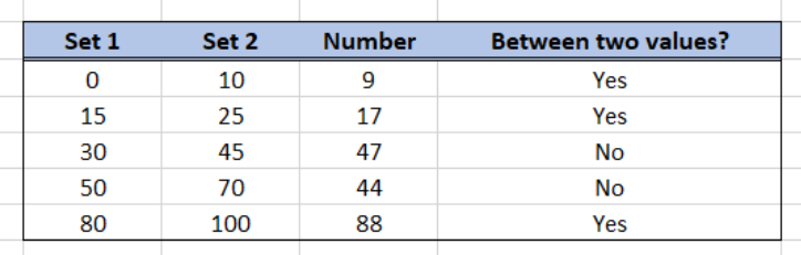 Figure 1. Final result: If number is between two values
Syntax of AND
=AND(logical1, [logical2], ...)
- Only logical1 is required while succeeding logical tests are optional
- logical1, logical2,…etc. are logical tests that the AND function will evaluate to be either TRUE or FALSE
Check if a number is between two values
In order to check if a number is between two values, we can use the AND function with two logical tests.
- Enter the formula in E4:
=AND(D4>B4,D4<C4)
The first logical test D4>B4 evaluates if the number is greater than the value in Set1, while the second logical test D4<C4 evaluates if the number is less than the value in Set2.
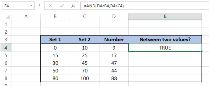 Figure 2. Entering the formula using AND
- Select E4 and drag the formula down to E8
As a result, we have determined that the number in rows 4, 5 and 8 are between the values in Set 1 and Set 2. For example, the number “9” in D4 is between the values 0 and 10. Hence, the AND function returns TRUE.
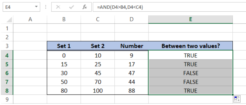 Figure 3. Output: If a number is between two values
However, there are times when the values we are comparing are interchanged and are not arranged in ascending order. Suppose we have below data wherein Set2 values are not always greater than the values in Set1.
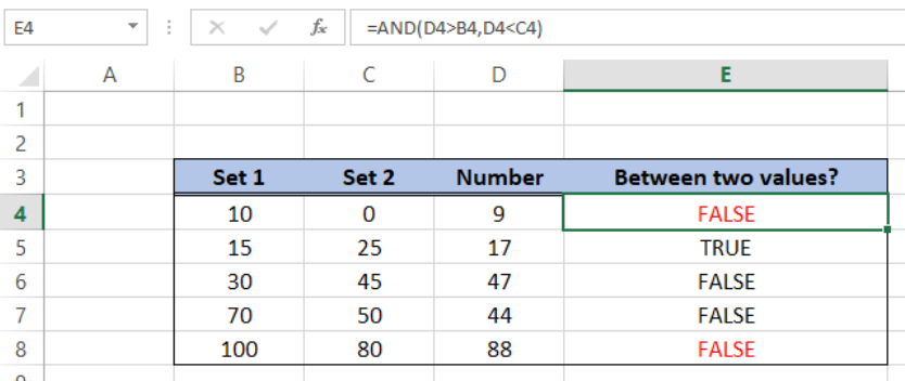 Figure 4. Erroneous results when values are interchanged
Using the same formula will yield erroneous results. Hence, we need to apply a formula that compares if a number is greater than the smaller value, and evaluates if a number is less than the larger value. This time we use the AND function with MIN and MAX.
Check if number is between two values using MIN and MAX
- Enter the formula in E4:
=AND(D4>(MIN(B4,C4)),D4<(MAX(B4,C4)))
- Select E4 and drag the formula down to E8
Our formula first compares the number with the smaller of the two values through the MIN function. Next, it compares the number with the larger of the two sets of values through the MAX function.
Below table shows the correct results when evaluating if a value is between two numbers in Set1 and Set2, regardless of which set contains the smaller or larger number.
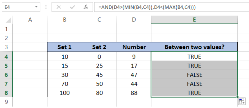 Figure 5. AND formula with MIN and MAX
IF statement between two numbers
We can customize the result when comparing values by using the IF function with the AND function. Suppose we want the formula to return “YES” if a number is between two values, and “NO” if otherwise.
- Enter the formula in E4:
=IF(AND(D4>(MIN(B4,C4)),D4<(MAX(B4,C4))),"Yes","No")
- Select E4 and drag the formula down to E8
We simply wrapped the IF function around the AND formula. As a result, the formula returns “Yes” instead of “TRUE”, and “No” instead of “FALSE”.
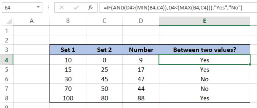 Figure 6. Output: IF statement between two numbers
Instant Connection to an Excel Expert
Most of the time, the problem you will need to solve will be more complex than a simple application of a formula or function. If you want to save hours of research and frustration, try our live Excelchat service! Our Excel Experts are available 24/7 to answer any Excel question you may have. We guarantee a connection within 30 seconds and a customized solution within 20 minutes.
There is no explicit Between formula in Excel, however, we can come up with creative ways to create this functionality. Our goal is to evaluate if a given value is between a range, for example, is 6 between 1 and 10?
We have three possible scenarios:
- Between formula in Excel for Numbers
- Between formula in Excel for Dates
- Between formula in Excel for Text
You can download this Excel Workbook and follow along:
DOWNLOAD EXCEL WORKBOOK
Between formula in Excel for Numbers
OPTION 1:Using a combination of MIN, MAX & AND function
In the example below, you have the start of the range in Column A, end of the range in Column B and the value to be evaluated in Column C.
You need to check whether the number entered in Column C is in between the numbers in Column A & Column B using a creatively formulated BETWEEN formula in Excel.

The function that can be used to determine if the value in cell D7 is in-between values in cell A7 & B7 is
=IF(AND(C7>=MIN(A7,B7),C7<=MAX(A7,B7)), “Yes”, “No”)
Let’s break this formula into parts to understand it better:
- C7 >= MIN(A7, B7) – This expression checks whether the value in cell C7 is greater than (or equal to) the smaller of the two numbers in cell A7 and B7.
- C7 <= MAX(A7, B7) – This expression checks whether the value in cell C7 is smaller than (or equal to) the larger of the two numbers in cell A7 and B7.
- AND( C7 >= MIN(A7, B7), C7 <= MAX(A7, B7)) – AND function simply checks whether the above two conditions are met or not i.e. whether the value in cell C7 is greater than (or equal to) the smaller number and less than (or equal to) the larger number.

OPTION 2:Using a MEDIAN function
You can use a simpler version of this complicated function by creatively using the Median formula:

=IF(C7=MEDIAN(A7:C7), “Yes”, “No”)
In our first example above, the range is 20-60, upon checking the value 50, it is in between this range.
The median formula will return the value in the middle of these 3 values when arranged in increasing order: 20, 50, 60. The median value is 50.
Since it matches the value we are evaluating, then the answer we get is a Yes, this value (50) is in between the range.
Now that you have learned how to use Excel if between two numbers, let’s move forward to dates and text.
Between formula in Excel for Dates
Irrespective of how you format a cell to display a date, Excel always stores it as a number. The number stored for each date actually represents the number of days since 0-Jan-1990.
1st Jan 1990 is stored as 1 (representing 1 day since 0-Jan-1990) and 23rd June 2020 is stored as 44,005 (representing 44005 days since 0-Jan-1990).
So, to check whether a date is in between two mentioned dates, we have the same application as the median formula.
Below is an example of how to use the median function to check dates.

=IF(C10=MEDIAN(A10:C10), “Yes”, “No”)
In our first example above, the range is May 1 – July 1, upon checking the date June 1, it is in between this range.
The median formula will return the value in the middle of these 3 dates when arranged in increasing order: May 1, June 1, July 1. The median value is June 1.
Since it matches the value we are evaluating, then the answer we get is a Yes, this value (June 1) is in between the range.
Between formula in Excel for Text
For text, we are checking if the value is alphabetically in the middle. We will be using the and formula:

=IF(AND(C12>=A12, C12<=B12, “Yes”, “No”)
Interestingly enough, you can compare texts using the >= and <= operators. Excel is able to compare them which goes alphabetically first or last.
In our first example above, the range is Cat – Dog, upon checking the text Cow, it is in between this range. As when arranged alphabetically, it would be: Cat, Cow, Dog.
The And formula checks if Cow >= Cat, and Cow <= Dog. You will see that both of these are true, as Cow is alphabetically later than Cat, while Cow is alphabetically ahead of Dog. Which is why we get a Yes result.
Conclusion
In this tutorial, you have learned how to use Between formula in Excel even when there is no explicit formula available to do this. You can use a combination of various other available function to create Excel if between range functionality.
You can use MIN, MAX, MEDIAN & AND functions to create a creative Between function in Excel for numbers, dates and text.
HELPFUL RESOURCE:

Make sure to download our FREE PDF on the 333 Excel keyboard Shortcuts here:
This tutorial will demonstrate how to highlight cells that contain a value between two other specified values in Excel and Google Sheets.
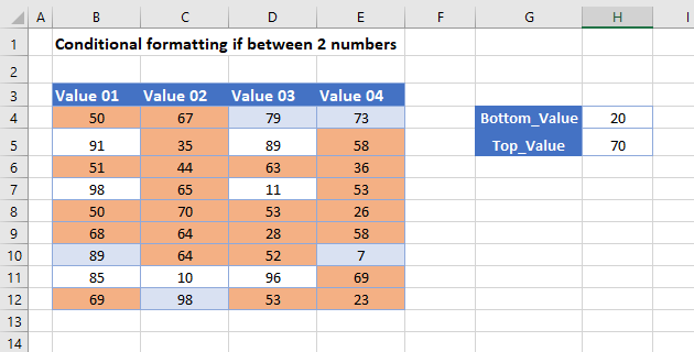
Conditional Formatting if Between Two Numbers
To highlight cells where the value is between a set minimum and maximum (inclusive), you can use one of the built-in Highlight Cell Rules within the Conditional Formatting menu.
- Select the range you want to apply formatting to.
- In the Ribbon, select Home > Conditional Formatting > Highlight Cells Rules > Between…
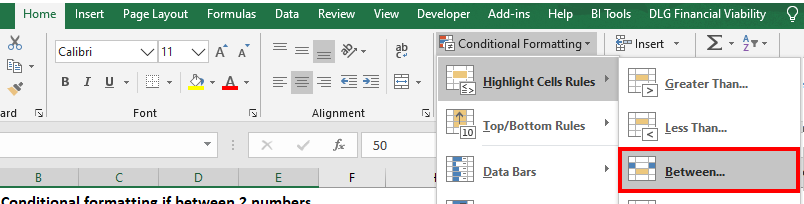
- You can either type in the bottom and top values, or to make the formatting dynamic (i.e., the result will change if you change the cells), click on the cells that contain the bottom and top values. Click OK.
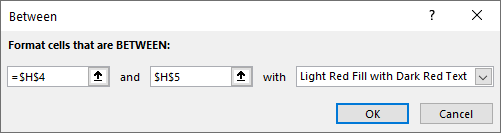
Values between 20 and 70 (inclusive) are highlighted.
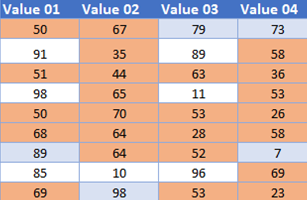
- When you change the two values in Cells H4 and H5, you obtain a different result.
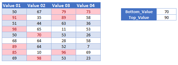
Alternate Method – Custom Formula
You can also highlight cells between two specified numbers by creating a New Rule and selecting Use a formula to determine which cells to format.
- Select New Rule from the Conditional Formatting menu.
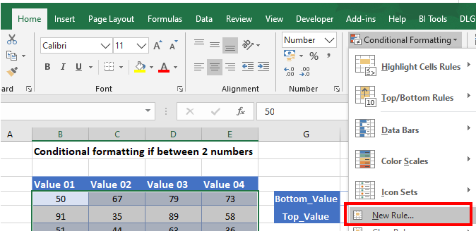
- Select Use a formula to determine which cells to format, and enter the formula (using the AND Function):
=AND(B4>=$H$4, B4<=$H$5)- The reference to cells H3 and H5 need to be locked by making them absolute. You can do this by using the $ sign around the row and column indicators, or by pressing F4 on the keyboard.
To learn more about how symbols are used in Excel, see How to Insert Signs and Symbols. - Click on the Format button.
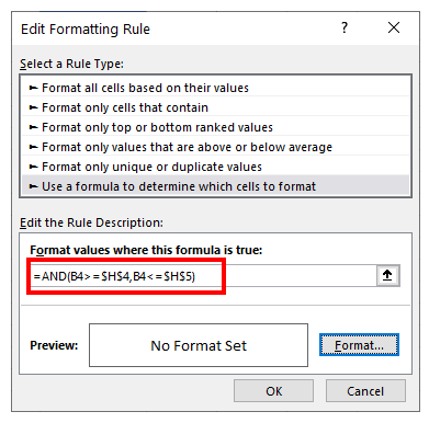
- Choose a fill color for the highlighted cells.
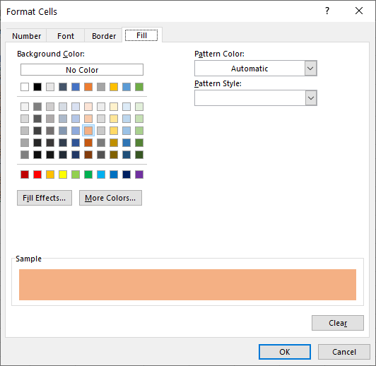
- Click OK, then OK again to return to the Conditional Formatting Rules Manager.
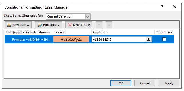
- Click Apply to apply the format to your worksheet.
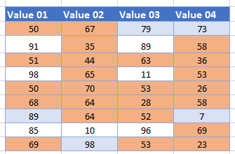
Highlight Cells Between Two Numbers in Google Sheets
Highlighting cells between two numbers in Google Sheets is similar.
- Highlight the cells you wish to format, and then click on Format > Conditional Formatting.
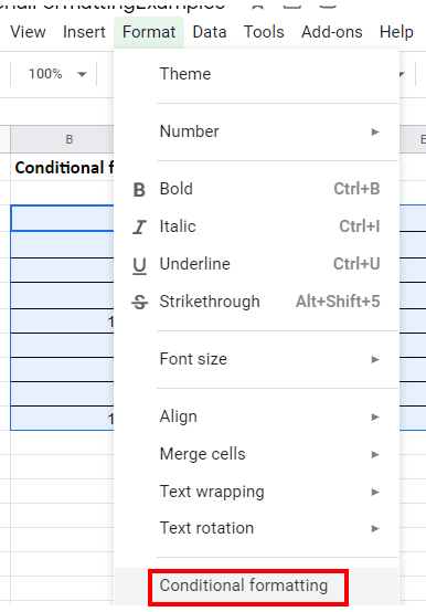
- The Apply to Range section will already be filled in.

- From the Format Rules section, select Is Between from the drop-down list and set the minimum and maximum values.
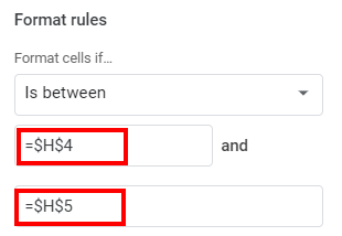
- Once again, you need to use the absolute signs (dollar signs) to lock in the values in Cells H4 and H5.
- Select the fill style for the cells that meet the criteria.
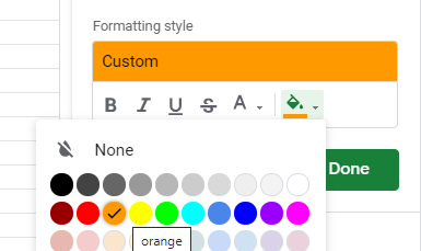
- Click Done to apply the rule.
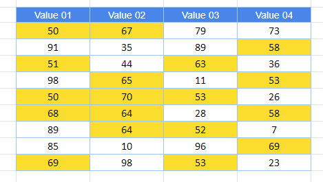
Custom Formula in Google Sheets
- To use a custom formula rather than a built-in rule, select Custom formula is under Format Rules, and type the formula.
=AND(B4>=$H$4, B4<=$H$5)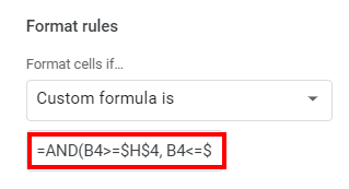
Remember to use $s or the F4 key to make Cells H4 and H5 absolute.
- Select your formatting and click Done.
In this article, we will learn how to check if the value is between the two numbers in Excel.
We have 2 numbers and a value to check that it lies between the given two numbers or not. For this article, we need to satisfy two conditions using AND logic operator. AND logic operator checks multiple conditions and returns TRUE only if all the condition stands TRUE or FALSE otherwise.
The two conditions which needed to check are The value must be smaller than the larger of the number and Greater than the smaller of the numbers. For this we will be using the MIN & MAX function in excel
Syntax:
=AND ( logic_test1, logic_test2,…)
Let’s learn this through an example shown below.
Here we have the two numbers given in Column A and Column B and the value to check in Column C.
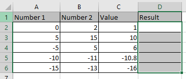
Use the formula
Explanation:
We just need to check 2 condition
- The value is greater than the smaller of the two numbers.
- The value is smaller than the larger of the two numbers.
Here MAX & MIN function returns the maximum and minimum of the two numbers. AND functions test both conditions and returns “True” only if both statements stands True else False.
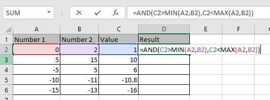
Press Enter and copy the formula in other cells using Ctrl + D shortcut.
As you can see the formula returns True if the value lies between the two numbers else it returns False.
Hope you learned how to check the value lies between the two numbers in Excel. Explore more articles here on Excel Logic_test functions here. Please feel free to state your query or feedback in the comment section below. We will help you.
Related Articles
How to Ignore zero in the Average of numbers in Excel
How to Get Random numbers between two numbers in Excel
How to Calculate a ratio of two numbers in Excel
How to Generate Random Phone Numbers in Excel
Popular Articles
50 Excel Shortcut to Increase Your Productivity
Edit a dropdown list
If with conditional formatting
If with wildcards
Vlookup by date