
Excel for Microsoft 365 Excel for Microsoft 365 for Mac Excel 2021 Excel 2021 for Mac Excel 2019 Excel 2019 for Mac Excel 2016 Excel 2016 for Mac Excel 2013 Excel 2010 Excel 2007 Excel for Mac 2011 More…Less
Sometimes you need to check if a cell is blank, generally because you might not want a formula to display a result without input.

In this case we’re using IF with the ISBLANK function:
-
=IF(ISBLANK(D2),»Blank»,»Not Blank»)
Which says IF(D2 is blank, then return «Blank», otherwise return «Not Blank»). You could just as easily use your own formula for the «Not Blank» condition as well. In the next example we’re using «» instead of ISBLANK. The «» essentially means «nothing».
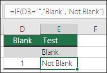
=IF(D3=»»,»Blank»,»Not Blank»)
This formula says IF(D3 is nothing, then return «Blank», otherwise «Not Blank»). Here is an example of a very common method of using «» to prevent a formula from calculating if a dependent cell is blank:
-
=IF(D3=»»,»»,YourFormula())
IF(D3 is nothing, then return nothing, otherwise calculate your formula).
Need more help?
Want more options?
Explore subscription benefits, browse training courses, learn how to secure your device, and more.
Communities help you ask and answer questions, give feedback, and hear from experts with rich knowledge.
Explanation
The COUNTIF function counts cells that meet criteria, returning the number of occurrences found. If no cells meet criteria, COUNTIF returns zero. You can use behavior directly inside an IF statement to mark values that have a zero count (i.e. values that are missing). In the example shown, the formula in G6 is:
=IF(COUNTIF(list,F6),"OK","Missing")
where «list» is a named range that corresponds to the range B6:B11.
The IF function requires a logical test to return TRUE or FALSE. In this case, the COUNTIF function performs the logical test. If the value is found in list, COUNTIF returns a number directly to the IF function. This result could be any number… 1, 2, 3, etc.
The IF function will evaluate any number as TRUE, causing IF to return «OK». If the value is not found in list, COUNTIF returns zero (0), which evaluates as FALSE, and IF returns «Missing».
Alternative with MATCH
You can also test for missing values using the MATCH function. MATCH finds the position of an item in a list and will return the #N/A error when a value is not found. You can use this behavior to build a formula that returns «Missing» or «OK» by testing the result of MATCH with the ISNA function. ISNA returns TRUE only when it receives the #N/A error.
To use MATCH as shown in the example above, the formula is:
=IF(ISNA(MATCH(F6,list,0)),"Missing","OK")

Note that MATCH must be configured for exact match. To do this, make sure the third argument is zero or FALSE.
Alternative with VLOOKUP
Since VLOOKUP also returns an #N/A error when a value isn’t round, you can build a formula with VLOOKUP that works the same as the MATCH option. As with MATCH, you must configure VLOOKUP to use exact match, then test the result with ISNA. Also note that we only give VLOOKUP a single column (column B) for the table array.

Return to Excel Formulas List
Download Example Workbook
Download the example workbook
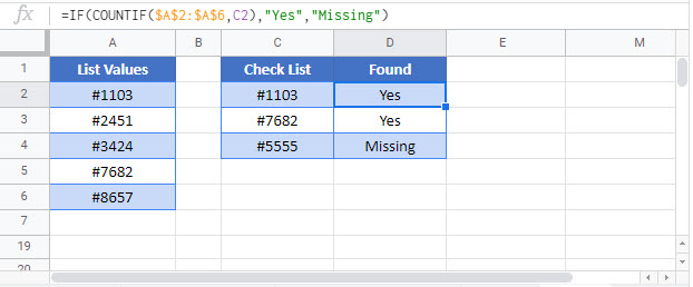
This tutorial will demonstrate how to check whether items are missing within a list in Excel and Google Sheets.
Find Missing Values
There are several ways to check if items are missing from a list.
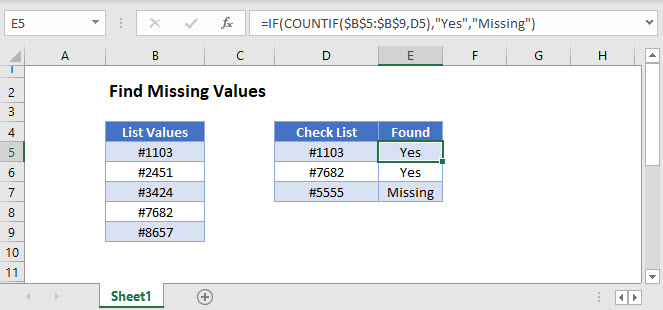
Find Missing Values with COUNTIF
One way to find missing values in a list is to use the COUNTIF Function together with the IF Function.
=IF(COUNTIF(B3:B7,D3),"Yes","Missing")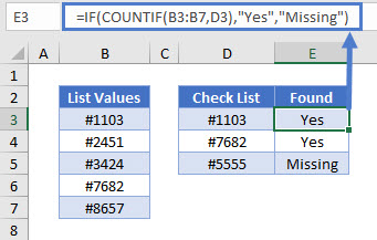
Let’s see how this formula works.
COUNTIF Function
The COUNTIF Function counts the number of cells that meet a given criterion. If no cells meet the condition, it returns zero.
=COUNTIF(B3:B7,D3)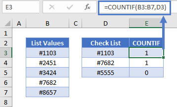
In this example, “#1103” and “#7682” are in Column B, so the formula gives us 1 for each. “#5555” is not in the list, so the formula gives us 0.
IF Function
The IF Function will evaluate any non-zero number as TRUE, and zero as FALSE.
Within the IF Function, we perform our count, then output “Yes” for TRUE and “No” for FALSE. This gives us our original formula of:
=IF(COUNTIF(B3:B7,D3),"Yes","Missing")
Find Missing Values with VLOOKUP
Another way to find missing values in a list is to use the VLOOKUP and ISNA Functions together with the IF Function.
=IF(ISNA(VLOOKUP(D3,B3:B7,1,FALSE)),"Missing","Yes")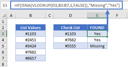
Let’s go through this formula.
VLOOKUP Function
Start by performing an exact-match VLOOKUP (FALSE) for the values in your list.
=VLOOKUP(D3,B3:B7,1,FALSE)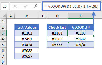
If the item is found, the VLOOKUP Function will return that item, otherwise it will return the #N/A error.
ISNA Function
You can use the ISNA Function to convert the #N/A errors to TRUE, indicating that those values are missing.
=ISNA(E3)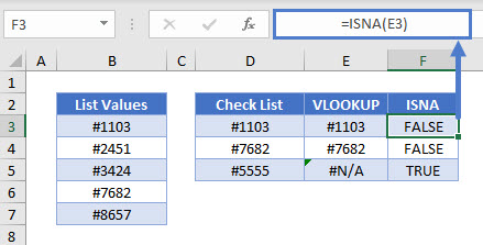
All non-error values result in FALSE.
IF Function
Then convert the results of the ISNA Function to show whether the value is missing. If the VLOOKUP Function gave us an error, the item is “Missing”.
=IF(F3,"Missing","Yes")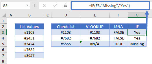
Item in both lists display “Yes”.
Combining these steps gives us the original formula:
=IF(ISNA(VLOOKUP(D3,B3:B7,1,FALSE)),"Missing","Yes")Find Missing Values in Google Sheets
These formulas work exactly the same in Google Sheets as in Excel.
If you want to search for the presence of a certain entry in a list then making a comparison of those entries with that of the list containing the data will be helpful. The formula presented in this article will make use of IF and COUNTIF statements.
Find Missing Values
Missing values from a list can be checked by using the COUNTIF function passed as a logical test to the IF function. After the logical test, if the entry is found then a string “OK” is returned otherwise “Missing” is returned.
Formula
=IF (COUNTIF(list,value),“OK”,“Missing”)
Explanation
To find the missing entries from a list, a conditional COUNT check is made which counts only if the condition passed to it becomes true. If this count check is true then the IF condition covering it intimates about the presence of that certain entry in the list.
How to Find the Missing Values
To find the missing values from a list, define the value to check for and the list to be checked inside a COUNTIF statement. If the value is found in the list then the COUNTIF statement returns the numerical value which represents the number of times the value occurs in that list.
The COUNTIF statement returns the results which play a role as the first argument of IF statement for the logical test to be performed. If the count returned by COUNTIF statement is zero then the IF statement returns that value which is passed when a logical test fails. In the other case, if COUNTIF statement returns some number IF statement is operated with a logical test to be true.
Example 1
An example sheet has been considered which has an array named as “list” containing serial numbers (Sr. No.). A separate search list has been made, which enlists the entries that are needed to be checked in the list. The sample sheet is shown below:
 Figure1. Sample sheet for finding the missing value
To find the missing value in the cell E3, enter the following formula in F3 to check its status.
=IF(COUNTIF(list,E3),"OK","MISSING")
 Figure2. Using the formula in F3 to look for the missing value (in E3) in the list (B3:B8)
The results of this formula can be observed in the snapshot below:
 Figure3. Updated status of missing and available values
It can be seen that the entries 1256 and 1260 are present in the array “list” as its 2nd and 4th entries respectively. Therefore, their status is updated as OK. While the entries 1258 and 1259 are not available and are updated as “MISSING”.
Alternative Formulae to Find Missing Values
Example 2
Missing values can also be found with the help of MATCH function. MATCH will look for the position of a certain item and will generate a #N/A error if the value is not found. This check can be passed as the logical test to the IF statement which will update the status of the entry accordingly. The generic formula for finding the missing values using the MATCH function is written below:
=IF(ISNA(MATCH(value,range,0)),"MISSING","OK")
The results obtained by this function are the same as shown below:
 Figure4. Using the MATCH function with ISNA and IF function to find missing values
Example 3
Missing values can also be found with the help of VLOOKUP function. VLOOKUP returns a #N/A error if a value is not found from the list. In place of MATCH function, VLOOKUP function is used here with ISNA function to find the missing values.
The following figure shows the results with VLOOKUP function with the formula mentioned in it:
 Figure5. Using the VLOOKUP function with ISNA and IF function to find missing values
17 авг. 2022 г.
читать 2 мин
Вы можете использовать следующую формулу в Excel для выполнения какой-либо задачи, если ячейка не пуста:
=IF( A1 <> "" , Value_If_Not_Empty, Value_If_Empty)
Эта конкретная формула проверяет, пуста ли ячейка A1 .
Если он не пустой, то возвращается Value_If_Not_Empty .
Если он пуст, возвращается значение Value_If_Empty .
В следующем примере показано, как использовать эту формулу на практике.
Пример: используйте формулу «Если не пусто» в Excel
Предположим, у нас есть следующий набор данных в Excel, который содержит информацию о различных баскетбольных командах:
![]()
Мы можем использовать следующую формулу, чтобы вернуть значение «Команда существует», если ячейка в столбце A не пуста.
В противном случае мы вернем значение «Не существует»:
=IF( A2 <> "" , "Team Exists", "Does Not Exist")
На следующем снимке экрана показано, как использовать эту формулу на практике:
![]()
Если имя команды не пусто в столбце А, возвращается «Команда существует».
В противном случае возвращается «Не существует».
Если бы мы хотели, мы могли бы также возвращать числовые значения вместо символьных значений.
Например, мы могли бы использовать следующую формулу, чтобы вернуть значение столбца очков, разделенное на два, если ячейка в столбце A не пуста.
В противном случае мы вернем пустое значение:
=IF( A2 <> "" , B2 / 2 , "" )
На следующем снимке экрана показано, как использовать эту формулу на практике:
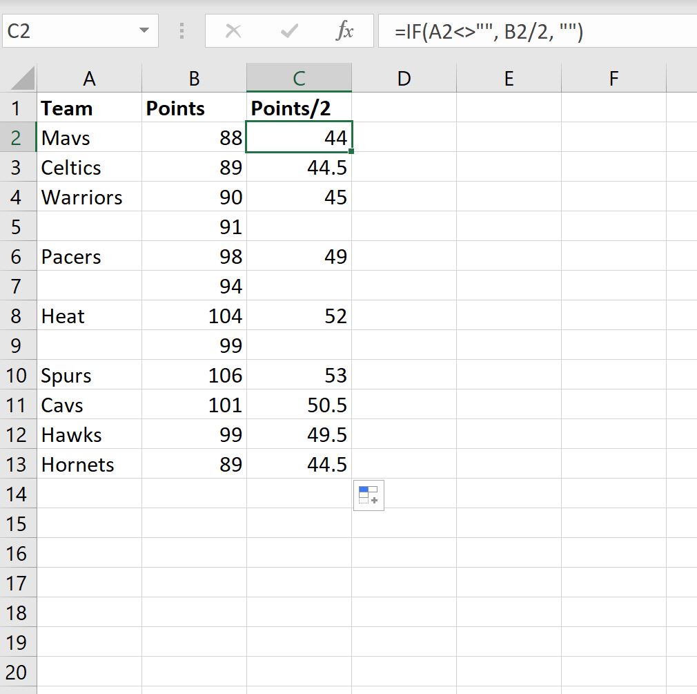
Если название команды не пусто в столбце A, то мы возвращаем значение в столбце очков, умноженное на два.
В противном случае мы возвращаем пустое значение.
Дополнительные ресурсы
В следующих руководствах объясняется, как выполнять другие распространенные задачи в Google Таблицах:
Как отфильтровать ячейки, содержащие текст, в Google Sheets
Как извлечь подстроку в Google Sheets
Как извлечь числа из строки в Google Sheets
Hello, Excellers welcome back for another Excel blog post in my 2020 series where I share my #FormulaFriday #Excel tips. Today let’s look at a really handy Excel formula or a number of formulas that will tell us what numbers are missing in a sequenced data set. Cool huh?. Let’s get writing that formula to find those missing values in Excel.
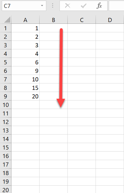
We are going to use a number of Excel formulas. We will begin with the logical IF Function. Here is my sample data set. I can clearly see that some of the numbers from 1 to 20 missing. But just which ones?.
Find The Missing Values In Excel.
Starting With The IF Function.
We start our formula with the IF Function which will test if a condition is met returning one value for TRUE and another for FALSE. We will need to test if we find an error (#N/A) or not. Which is why we first then use the ISNA function which checks if a value is #N/A and returns TRUE or FALSE. So here is the first part of our formula set up.
Bring In The VLOOKUP Function.
Next, we take the VLOOKUP Function to lookup the ROW number that relates to cell A1 (which returns the value 1) in the list of values that are in cells A1 to A20. We are looking to see if the VLOOKUP returns #N/A.

Finishing The IF Function.
We now specify what we need to display in the cell if the row number is not found. This is the ‘value if true’ part of the IF Function. We specify that we find #N/A then Excel must return the row number.
If the result of the VLOOKUP Function is not #N/A and the row number is found then we simply get Excel to return a blank cell using the double quotes ” “.

Dragging The Excel Formula.
So, my final stage of the formula is to simply drag the formula to row 20 to allow Excel to see what rows up to and including 20 are missing. Sweet. How cool is that?. See the results below. Excel has identified exactly which of the values are missing. Have you used this method before or another way?. Share in the comment below. Would you use MATCH Function or how about some Excel VBA code?.
That’s it. A cool way to fill missing values in Excel.
What Next? Want More Excel Tips?

So, if you want more top tips then sign up for my Monthly Newsletter where I share 3 Tips on the first Wednesday of the month and receive my free Ebook, 30 Excel Tips.
A Full list Of Formula Friday Blog Posts


Do You Need Help With An Excel Problem?.
Finally, I am pleased to announce I have teamed up with Excel Rescue, where you can get help FAST.

Проверка переменных и выражений с помощью встроенных функций VBA Excel: IsArray, IsDate, IsEmpty, IsError, IsMissing, IsNull, IsNumeric, IsObject.
Проверка переменных и выражений
Встроенные функции VBA Excel — IsArray, IsDate, IsEmpty, IsError, IsMissing, IsNull, IsNumeric, IsObject — проверяют значения переменных и выражений на соответствие определенному типу данных или специальному значению.
Синтаксис функций для проверки переменных и выражений:
Expression — выражение, переменная или необязательный аргумент для IsMissing.
Все функции VBA Excel для проверки переменных и выражений являются логическими и возвращают значение типа Boolean — True или False.
Функция IsArray
Описание функции
Функция IsArray возвращает значение типа Boolean, указывающее, является ли переменная массивом:
- True — переменная является массивом;
- False — переменная не является массивом.
Пример с IsArray
|
Sub Primer1() Dim arr1(), arr2(1 To 10), arr3 Debug.Print IsArray(arr1) ‘Результат: True Debug.Print IsArray(arr2) ‘Результат: True Debug.Print IsArray(arr3) ‘Результат: False arr3 = Array(1, 2, 3, 4, 5) Debug.Print IsArray(arr3) ‘Результат: True End Sub |
Как показывает пример, функция IsArray возвращает True и в том случае, если переменная только объявлена как массив, но еще не содержит значений.
Функция IsDate
Описание функции
Функция IsDate возвращает логическое значение, указывающее, содержит ли переменная значение, которое можно интерпретировать как дату:
- True — переменная содержит дату, выражение возвращает дату, переменная объявлена с типом As Date;
- False — в иных случаях.
Пример с IsDate
|
Sub Primer2() Dim d1 As String, d2 As Date Debug.Print IsDate(d1) ‘Результат: False Debug.Print IsDate(d2) ‘Результат: True d1 = «14.01.2023» Debug.Print IsDate(d1) ‘Результат: True Debug.Print IsDate(Now) ‘Результат: True End Sub |
Функция IsEmpty
Описание функции
Функция IsEmpty возвращает значение типа Boolean, указывающее, содержит ли переменная общего типа (As Variant) значение Empty:
- True — переменная содержит значение Empty;
- False — переменной присвоено значение, отличное от Empty.
Пример с IsEmpty
|
Sub Primer3() Dim s As String, v As Variant Debug.Print IsEmpty(s) ‘Результат: False Debug.Print IsEmpty(v) ‘Результат: True v = 125 Debug.Print IsEmpty(v) ‘Результат: False Range(«A1»).Clear Debug.Print IsEmpty(Range(«A1»)) ‘Результат: True Range(«A1») = 123 Debug.Print IsEmpty(Range(«A1»)) ‘Результат: False End Sub |
Как видно из примера, функцию IsEmpty можно использовать для проверки ячеек на содержание значения Empty (пустая ячейка общего формата).
Функция IsError
Описание функции
Функция IsError возвращает логическое значение, указывающее, является ли аргумент функции значением ошибки, определенной пользователем:
- True — аргумент функции является значением ошибки, определенной пользователем;
- False — в иных случаях.
Пользователь может определить одну или несколько ошибок для своей процедуры или функции с рекомендациями действий по ее (их) исправлению. Возвращается номер ошибки с помощью функции CVErr.
Пример с IsError
Допустим, пользователь определил, что ошибка №25 означает несоответствие аргумента функции Vkuba числовому формату:
|
Function Vkuba(x) If IsNumeric(x) Then Vkuba = x ^ 3 Else Vkuba = CVErr(25) End If End Function Sub Primer4() Debug.Print Vkuba(5) ‘Результат: 125 Debug.Print IsError(Vkuba(5)) ‘Результат: False Debug.Print Vkuba(«пять») ‘Результат: Error 25 Debug.Print IsError(Vkuba(«пять»)) ‘Результат: True End Sub |
Функция IsMissing
Описание функции
Функция IsMissing возвращает значение типа Boolean, указывающее, был ли необязательный аргумент типа данных Variant передан процедуре:
- True — если в процедуру не было передано значение для необязательного аргумента;
- False — значение для необязательного аргумента было передано в процедуру.
Пример с IsMissing
|
Function Scepka(x, Optional y) If Not IsMissing(y) Then Scepka = x & y Else Scepka = x & » (а необязательный аргумент не подставлен)» End If End Function Sub Primer5() Debug.Print Scepka(«Тропинка», » в лесу») ‘Результат: Тропинка в лесу Debug.Print Scepka(«Тропинка») ‘Результат: Тропинка (а необязательный аргумент не подставлен) End Sub |
Функция IsNull
Описание функции
Функция IsNull возвращает логическое значение, указывающее, является ли Null значением переменной или выражения:
- True — значением переменной или выражения является Null;
- False — в иных случаях.
Пример с IsNull
Функция IsNull особенно необходима из-за того, что любое условие с выражением, в которое входит ключевое слово Null, возвращает значение False:
|
Sub Primer6() Dim Var Var = Null If Var = Null Then Debug.Print Var ‘Результат: «» If Var <> Null Then Debug.Print Var ‘Результат: «» If IsNull(Var) Then Debug.Print Var ‘Результат: Null End Sub |
Функция IsNumeric
Описание функции
Функция IsNumeric возвращает значение типа Boolean, указывающее, можно ли значение выражения или переменной рассматривать как число:
- True — если аргумент функции может рассматриваться как число;
- False — в иных случаях.
Пример с IsNumeric
|
Sub Primer7() Debug.Print IsNumeric(«3,14») ‘Результат: True Debug.Print IsNumeric(«четыре») ‘Результат: False End Sub |
Функция IsObject
Описание функции
Функция IsObject возвращает логическое значение, указывающее, является ли переменная объектной:
- True — переменная содержит ссылку на объект или значение Nothing;
- False — в иных случаях.
Функция IsObject актуальна для переменных типа Variant, которые могут содержать как ссылки на объекты, так и значения других типов данных.
Пример с IsObject
|
Sub Primer8() Dim myObj As Object, myVar As Variant Debug.Print IsObject(myObj) ‘Результат: True Debug.Print IsObject(myVar) ‘Результат: False Set myVar = ActiveSheet Debug.Print IsObject(myVar) ‘Результат: True End Sub |
I’ve got a range (A3:A10) that contains names, and I’d like to check if the contents of another cell (D1) matches one of the names in my list.
I’ve named the range A3:A10 ‘some_names’, and I’d like an excel formula that will give me True/False or 1/0 depending on the contents.
asked May 29, 2013 at 20:43
![]()
joseph.hainlinejoseph.hainline
2,0523 gold badges16 silver badges16 bronze badges
=COUNTIF(some_names,D1)
should work (1 if the name is present — more if more than one instance).
answered May 29, 2013 at 20:47
![]()
1
My preferred answer (modified from Ian’s) is:
=COUNTIF(some_names,D1)>0
which returns TRUE if D1 is found in the range some_names at least once, or FALSE otherwise.
(COUNTIF returns an integer of how many times the criterion is found in the range)
![]()
pnuts
6,0623 gold badges27 silver badges41 bronze badges
answered Jun 6, 2013 at 20:40
![]()
joseph.hainlinejoseph.hainline
2,0523 gold badges16 silver badges16 bronze badges
0
I know the OP specifically stated that the list came from a range of cells, but others might stumble upon this while looking for a specific range of values.
You can also look up on specific values, rather than a range using the MATCH function. This will give you the number where this matches (in this case, the second spot, so 2). It will return #N/A if there is no match.
=MATCH(4,{2,4,6,8},0)
You could also replace the first four with a cell. Put a 4 in cell A1 and type this into any other cell.
=MATCH(A1,{2,4,6,8},0)
![]()
answered Nov 10, 2014 at 22:57
![]()
RPh_CoderRPh_Coder
4784 silver badges4 bronze badges
6
If you want to turn the countif into some other output (like boolean) you could also do:
=IF(COUNTIF(some_names,D1)>0, TRUE, FALSE)
Enjoy!
answered May 29, 2013 at 21:09
![]()
1
For variety you can use MATCH, e.g.
=ISNUMBER(MATCH(D1,A3:A10,0))
answered May 29, 2013 at 23:28
![]()
barry houdinibarry houdini
10.8k1 gold badge20 silver badges25 bronze badges
there is a nifty little trick returning Boolean in case range some_names could be specified explicitly such in "purple","red","blue","green","orange":
=OR("Red"={"purple","red","blue","green","orange"})
Note this is NOT an array formula
answered Jul 11, 2018 at 22:06
![]()
gregVgregV
2042 silver badges4 bronze badges
1
You can nest --([range]=[cell]) in an IF, SUMIFS, or COUNTIFS argument. For example, IF(--($N$2:$N$23=D2),"in the list!","not in the list"). I believe this might use memory more efficiently.
Alternatively, you can wrap an ISERROR around a VLOOKUP, all wrapped around an IF statement. Like, IF( ISERROR ( VLOOKUP() ) , "not in the list" , "in the list!" ).
answered Dec 5, 2013 at 19:33
![]()
0
In situations like this, I only want to be alerted to possible errors, so I would solve the situation this way …
=if(countif(some_names,D1)>0,"","MISSING")
Then I’d copy this formula from E1 to E100. If a value in the D column is not in the list, I’ll get the message MISSING but if the value exists, I get an empty cell. That makes the missing values stand out much more.
![]()
answered Aug 24, 2013 at 11:59
![]()
0
Array Formula version (enter with Ctrl + Shift + Enter):
=OR(A3:A10=D1)
answered Dec 8, 2016 at 12:38
![]()
SlaiSlai
1195 bronze badges
1
There are many ways to force excel for calculating a formula only if given cell/s are not blank. In this article, we will explore all the methods of calculating only «if not blank» condition.
So to demonstrate all the cases, I have prepared below data

In row 4, I want the difference of months of years 2109 and 2018. For that, I will subtract 2018’s month’s data from 2019’s month’s data. The condition is, if either cell is blank, there should be no calculation. Let’s explore in how many ways you can force excel, if cell is not blank.
Calculate If Not Blank using IF function with OR Function.
The first function we think of is IF function, when it comes to conditional output. In this example, we will use IF and OR function together.
So if you want to calculate if all cells are non blank then use below formula.
Write this formula in cell B4 and fill right (CTRL+R).
=IF(OR(B3=»»,B2=»»),»»,B2-B3)
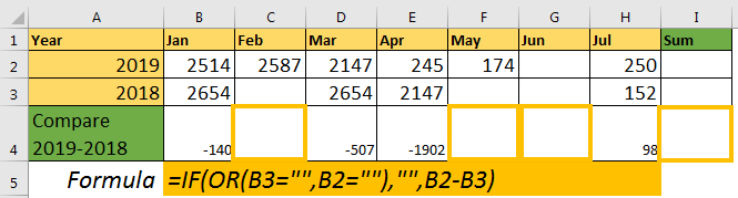
How Does It work?
The OR function checks if B3 and B2 are blank or not. If either of the cell is blank, it returns TRUE. Now, for True, IF is printing “” (nothing/blank) and for False, it is printing the calculation.
The same thing can be done using IF with AND function, we just need to switch places of True Output and False Output.
=IF(AND(B3<>»»,B2<>»»),B2-B3,»»)
In this case, if any of the cells is blank, AND function returns false. And then you know how IF treats the false output.
Using the ISBLANK function
In the above formula, we are using cell=”” to check if the cell is blank or not. Well, the same thing can be done using the ISBLANK function.
=IF(OR(ISBLANK(B3),ISBLANK(B2)),””,B2-B3)
It does the same “if not blank then calculate” thing as above. It’s just uses a formula to check if cell is blank or not.
Calculate If Cell is Not Blank Using COUNTBLANK
In above example, we had only two cells to check. But what if we want a long-range to sum, and if the range has any blank cell, it should not perform calculation. In this case we can use COUNTBLANK function.
=IF(COUNTBLANK(B2:H2),»»,SUM(B2:H2))
Here, count blank returns the count blank cells in range(B2:H2). In excel, any value grater then 0 is treated as TRUE. So, if ISBLANK function finds a any blank cell, it returns a positive value. IF gets its check value as TRUE. According to the above formula, if prints nothing, if there is at least one blank cell in the range. Otherwise, the SUM function is executed.
Using the COUNTA function
If you know, how many nonblank cells there should be to perform an operation, then COUNTA function can also be used.
For example, in range B2:H2, I want to do SUM if none of the cells are blank.
So there is 7 cell in B2:H2. To do calculation only if no cells are blank, I will write below formula.
=IF(COUNTA(B3:H3)=7,SUM(B3:H3),»»)
As we know, COUNTA function returns a number of nonblank cells in the given range. Here we check the non-blank cell are 7. If they are no blank cells, the calculation takes place otherwise not.
This function works with all kinds of values. But if you want to do operation only if the cells have numeric values only, then use COUNT Function instead.
So, as you can see that there are many ways to achieve this. There’s never only one path. Choose the path that fits for you. If you have any queries regarding this article, feel free to ask in the comments section below.
Related Articles:
How to Calculate Only If Cell is Not Blank in Excel
Adjusting a Formula to Return a Blank
Checking Whether Cells in a Range are Blank, and Counting the Blank Cells
SUMIF with non-blank cells
Only Return Results from Non-Blank Cells
Popular Articles
50 Excel Shortcut to Increase Your Productivity : Get faster at your task. These 50 shortcuts will make you work even faster on Excel.
How to use the VLOOKUP Function in Excel : This is one of the most used and popular functions of excel that is used to lookup value from different ranges and sheets.
How to use the COUNTIF function in Excel : Count values with conditions using this amazing function. You don’t need to filter your data to count specific values. Countif function is essential to prepare your dashboard.
How to use the SUMIF Function in Excel : This is another dashboard essential function. This helps you sum up values on specific conditions.