If not isna excel - Word и Excel - помощь в работе с программами

Excel for Microsoft 365 Excel for Microsoft 365 for Mac Excel for the web Excel 2021 Excel 2021 for Mac Excel 2019 Excel 2019 for Mac Excel 2016 Excel 2016 for Mac Excel 2013 Excel Web App Excel 2010 Excel 2007 Excel for Mac 2011 Excel Starter 2010 More…Less

Description

Each of these functions, referred to collectively as the IS functions, checks the specified value and returns TRUE or FALSE depending on the outcome. For example, the ISBLANK function returns the logical value TRUE if the value argument is a reference to an empty cell; otherwise it returns FALSE.

You can use an IS function to get information about a value before performing a calculation or other action with it. For example, you can use the ISERROR function in conjunction with the IF function to perform a different action if an error occurs:

=
IF(
ISERROR(A1), «An error occurred.», A1 * 2)

This formula checks to see if an error condition exists in A1. If so, the IF function returns the message «An error occurred.» If no error exists, the IF function performs the calculation A1*2.

Syntax

ISBLANK(value)

ISERR(value)

ISERROR(value)

ISLOGICAL(value)

ISNA(value)

ISNONTEXT(value)

ISNUMBER(value)

ISREF(value)

ISTEXT(value)

The IS function syntax has the following argument:

value Required. The value that you want tested. The value argument can be a blank (empty cell), error, logical value, text, number, or reference value, or a name referring to any of these.

Function	Returns TRUE if
ISBLANK	Value refers to an empty cell.
ISERR	Value refers to any error value except #N/A.
ISERROR	Value refers to any error value (#N/A, #VALUE!, #REF!, #DIV/0!, #NUM!, #NAME?, or #NULL!).
ISLOGICAL	Value refers to a logical value.
ISNA	Value refers to the #N/A (value not available) error value.
ISNONTEXT	Value refers to any item that is not text. (Note that this function returns TRUE if the value refers to a blank cell.)
ISNUMBER	Value refers to a number.
ISREF	Value refers to a reference.
ISTEXT	Value refers to text.

Remarks

The value arguments of the IS functions are not converted. Any numeric values that are enclosed in double quotation marks are treated as text. For example, in most other functions where a number is required, the text value «19» is converted to the number 19. However, in the formula ISNUMBER(«19»), «19» is not converted from a text value to a number value, and the ISNUMBER function returns FALSE.
The IS functions are useful in formulas for testing the outcome of a calculation. When combined with the IF function, these functions provide a method for locating errors in formulas (see the following examples).

Examples

Example 1

Copy the example data in the following table, and paste it in cell A1 of a new Excel worksheet. For formulas to show results, select them, press F2, and then press Enter. If you need to, you can adjust the column widths to see all the data.

Formula	Description	Result
=ISLOGICAL(TRUE)	Checks whether TRUE is a logical value	TRUE
=ISLOGICAL(«TRUE»)	Checks whether «TRUE» is a logical value	FALSE
=ISNUMBER(4)	Checks whether 4 is a number	TRUE
=ISREF(G8)	Checks whether G8 is a valid reference	TRUE
=ISREF(XYZ1)	Checks whether XYZ1 is a valid reference	FALSE

Example 2

Data
Gold
Region1
#REF!
330.92
#N/A
Formula	Description	Result
=ISBLANK(A2)	Checks whether cell A2 is blank.	FALSE
=ISERROR(A4)	Checks whether the value in cell A4, #REF!, is an error.	TRUE
=ISNA(A4)	Checks whether the value in cell A4, #REF!, is the #N/A error.	FALSE
=ISNA(A6)	Checks whether the value in cell A6, #N/A, is the #N/A error.	TRUE
=ISERR(A6)	Checks whether the value in cell A6, #N/A, is an error.	FALSE
=ISNUMBER(A5)	Checks whether the value in cell A5, 330.92, is a number.	TRUE
=ISTEXT(A3)	Checks whether the value in cell A3, Region1, is text.	TRUE

Need more help?

Источник

Return value

A logical value (TRUE or FALSE)

Usage notes

The ISNA function returns TRUE when a cell contains the #N/A error and FALSE for any other value, or any other error type. The ISNA function takes one argument, value, which is typically a cell reference.

Examples

If A1 contains the #N/A error, ISNA returns TRUE:

=ISNA(A1) // returns TRUE

ISNA returns FALSE for other values and errors:

=ISNA(100) // returns FALSE
=ISNA(5/0) // returns FALSE

You can use the ISNA function with the IF function test for #N/A and display a friendly message if the error occurs. For example, to display a message if A1 contains #N/A and the value of A1 if not:

=IF(ISNA(A1),"message",A1)

The IFNA function is a more efficient way to trap the #N/A error. See VLOOKUP without NA error for an example.

Return #N/A

To explicitly return the #N/A error in a formula, you can use the NA function:

=NA() // returns #N/A error

The following will return true:

=ISNA(NA()) // returns TRUE

Count #N/A errors

To count cells in a range that contain #N/A errors, you can use the SUMPRODUCT function like this:

=SUMPRODUCT(--ISNA(range))

The double negative coerces the TRUE and FALSE results from ISNA into 1s and 0s and SUMPRODUCT sums the result.

Notes

The IFNA function is a more efficient way to trap and handle the #N/A error.

Источник

Date yes Add (Subtract) Days to a Date Concatenate Dates Convert Date to Number Convert Date to Text Month Name to Number Create Date Range from Dates Day Number of Year Month Name from Date First Day of Month Add (Subtract) Weeks to a Date If Functions with Dates Max Date Number of Days Between Dates Number of Days in a Month Number of Weeks Between Dates Number of Years Between Dates Split Date & Time into Separate Cells Countdown Remaining Days Insert Dates Random Date Generator Using Dynamic Ranges — Year to Date Values Add (Subtract) Years to a Date Date Formula Examples Extract Day from Date Get Day Name from Date Count Days Left in Month / Year Count Workdays Left in Month / Year Get Last Day of Month Last Business Day of Month / Year Number of Work / Business Days in Month Weekday Abbreviations Auto Populate Dates Number of Months Between Dates Quarter from a Date Years of Service Change Date Format Compare Dates Time yes Add (Subtract) Hours to Time Add (Subtract) Minutes to Time Add (Subtract) Seconds to Time Add Up time (Total Time) Time Differences Change Time Format Convert Minutes to Hours Convert Time to Decimal Convert Time to Hours Convert Time to Minutes Convert Time to Seconds Military Time Round Time to Nearest 15 Minutes Overtime Calculator Number of Hours Between Times Convert Seconds to Minutes, Hours, or Time Count Hours Worked Time Differences Time Format — Show Minutes Seconds Text yes Add Commas to Cells Get First Word from Text Capitalize First Letter Clean & Format Phone #s Remove Extra Trailing / Leading Spaces Add Spaces to Cell Assign Number Value to Text Combine Cells with Comma Combine First and Last Names Convert Text String to Date Convert Text to Number Extract Text From Cell Get Last Word Remove Unwated Characters Extract Text Before or After Character How to Split Text String by Space, Comma, & More Remove Special Characters Remove First Characters from Left Substitute Multiple Values Switch First & Last Names w/ Commas Remove Specific Text from a Cell Extract Text Between Characters (Ex. Parenthesis) Add Leading Zeros to a Number Remove Line Breaks from Text Remove all Numbers from Text Reverse Text Remove Non-Numeric Characters Remove Last Character(s) From Right Separate First and Last Names Separate Text & Numbers Round yes Round Formulas Round Price to Nearest Dollar or Cent Round to Nearest 10, 100, or 1000 Round to Nearest 5 or .5 Round Percentages Round to Significant Figures Count yes Count Blank and Non-blank Cells Count Cells Between Two Numbers Count Cells not Equal to Count if Cells are in Range Count Times Word Appears in Cell Count Words in Cell Count Specific Characters in Column Count Total Number of Characters in Column Count Cells that Equal one of two Results Count Cells that do not Contain Count Cells that Contain Specific Text Count Unique Values in Range Countif — Multiple Criteria Count Total Number of Cells in Range Count Cells with Any Text Count Total Cells in a Table Lookup yes Two Dimensional VLOOKUP VLOOKUP Simple Example Vlookup — Multiple Matches Case Sensitive Lookup Case Sensitive VLOOKUP Sum if — VLOOKUP Case Sensitive Lookup Case Sensitive VLOOKUP Find Duplicates w/ VLOOKUP or MATCH INDEX MATCH MATCH Lookup — Return Cell Address (Not Value) Lookup Last Value in Column or Row Reverse VLOOKUP (Right to Left) Risk Score Bucket with VLOOKUP Sum with a VLOOKUP Function VLOOKUP & INDIRECT VLOOKUP Concatenate VLOOKUP Contains (Partial Match) 17 Reasons Why Your XLOOKUP is Not Working Double (Nested) XLOOKUP — Dynamic Columns IFERROR (& IFNA) XLOOKUP Lookup Min / Max Value Nested VLOOKUP Top 11 Alternatives to VLOOKUP (Updated 2022!) VLOOKUP – Dynamic Column Reference VLOOKUP – Fix #N/A Error VLOOKUP – Multiple Sheets at Once VLOOKUP & HLOOKUP Combined VLOOKUP & MATCH Combined VLOOKUP Between Worksheets or Spreadsheets VLOOKUP Duplicate Values VLOOKUP Letter Grades VLOOKUP Return Multiple Columns VLOOKUP Returns 0? Return Blank Instead VLOOKUP w/o #N/A Error XLOOKUP Multiple Sheets at Once XLOOKUP Between Worksheets or Spreadsheets XLOOKUP by Date XLOOKUP Duplicate Values XLOOKUP Multiple Criteria XLOOKUP Return Multiple Columns XLOOKUP Returns 0? Return Blank Instead XLOOKUP Text XLOOKUP with IF XLOOKUP With If Statement Misc. yes Sort Multiple Columns Use Cell Value in Formula Percentage Change Between Numbers Percentage Breakdown Rank Values Add Spaces to Cell CAGR Formula Average Time Decimal Part of Number Integer Part of a Number Compare Items in a List Dealing with NA() Errors Get Worksheet Name Wildcard Characters Hyperlink to Current Folder Compound Interest Formula Percentage Increase Create Random Groups Sort with the Small and Large Functions Non-volatile Function Alternatives Decrease a Number by a Percentage Calculate Percent Variance Profit Margin Calculator Convert Column Number to Letter Get Full Address of Named Range Insert File Name Insert Path Latitute / Longitude Functions Replace Negative Values Reverse List Range Convert State Name to Abbreviation Create Dynamic Hyperlinks Custom Sort List with Formula Data Validation — Custom Formulas Dynamic Sheet Reference (INDIRECT) Reference Cell in Another Sheet or Workbook Get Cell Value by Address Get Worksheet Name Increment Cell Reference List Sheet Names List Skipped Numbers in Sequence Return Address of Max Value in Range Search by Keywords Select Every Other (or Every nth) Row Basics yes Cell Reference Basics — A1, R1C1, 3d, etc. Add Up (Sum) Entire Column or Row Into to Dynamic Array Formulas Conversions yes Convert Time Zones Convert Celsius to Fahrenheit Convert Pounds to Kilograms Convert Time to Unix Time Convert Feet to Meters Convert Centimeters to Inches Convert Kilometers to Miles Convert Inches to Feet Convert Date to Julian Format Convert Column Letter to Number Tests yes Test if a Range Contains any Text Test if any Cell in Range is Number Test if a Cell Contains a Specific Value Test if Cell Contains Any Number Test if Cell Contains Specific Number Test if Cell is Number or Text If yes Percentile If Subtotal If Sumproduct If Large If and Small If Median If Concatentate If Max If Rank If TEXTJOIN If Sum yes Sum if — Begins With / Ends With Sum if — Month or Year to Date Sum if — By Year Sum if — Blank / Non-Blank Sum if — Horizontal Sum Count / Sum If — Cell Color INDIRECT Sum Sum If — Across Multiple Sheets Sum If — By Month Sum If — Cells Not Equal To Sum If — Not Blank Sum if — Between Values Sum If — Week Number Sum Text Sum if — By Category or Group Sum if — Cell Contains Specific Text (Wildcards) Sum if — Date Rnage Sum if — Dates Equal Sum if — Day of Week Sum if — Greater Than Sum if — Less Than Average yes Average Non-Zero Values Average If — Not Blank Average — Ignore 0 Average — Ignore Errors Math yes Multiplication Table Cube Roots nth Roots Square Numbers Square Roots Calculations yes Calculate a Ratio Calculate Age KILLLLLLL Calculate Loan Payments GPA Formula Calculate VAT Tax How to Grade Formulas Find yes Find a Number in a Column / Workbook Find Most Frequent Numbers Find Smallest n Values Find nth Occurance of Character in Text Find and Extract Number from String Find Earliest or Latest Date Based on Criteria Find First Cell with Any Value Find Last Row Find Last Row with Data Find Missing Values Find Largest n Values Most Frequent Number Conditional Formatting yes Conditional Format — Dates & Times Conditional Format — Highlight Blank Cells New Functions XLOOKUP Replaces VLOOKUP, HLOOKUP, and INDEX / MATCH Logical yes AND Checks whether all conditions are met. TRUE/FALSE IF If condition is met, do something, if not, do something else. IFERROR If result is an error then do something else. NOT Changes TRUE to FALSE and FALSE to TRUE. OR Checks whether any conditions are met. TRUE/FALSE XOR Checks whether one and only one condition is met. TRUE/FALSE Lookup & Reference yes FALSE The logical value: FALSE. TRUE The logical value: TRUE. ADDRESS Returns a cell address as text. AREAS Returns the number of areas in a reference. CHOOSE Chooses a value from a list based on it’s position number. COLUMN Returns the column number of a cell reference. COLUMNS Returns the number of columns in an array. HLOOKUP Lookup a value in the first row and return a value. HYPERLINK Creates a clickable link. INDEX Returns a value based on it’s column and row numbers. INDIRECT Creates a cell reference from text. LOOKUP Looks up values either horizontally or vertically. MATCH Searches for a value in a list and returns its position. OFFSET Creates a reference offset from a starting point. ROW Returns the row number of a cell reference. ROWS Returns the number of rows in an array. TRANSPOSE Flips the oriention of a range of cells. VLOOKUP Lookup a value in the first column and return a value. Date & Time yes DATE Returns a date from year, month, and day. DATEDIF Number of days, months or years between two dates. DATEVALUE Converts a date stored as text into a valid date DAY Returns the day as a number (1-31). DAYS Returns the number of days between two dates. DAYS360 Returns days between 2 dates in a 360 day year. EDATE Returns a date, n months away from a start date. EOMONTH Returns the last day of the month, n months away date. HOUR Returns the hour as a number (0-23). MINUTE Returns the minute as a number (0-59). MONTH Returns the month as a number (1-12). NETWORKDAYS Number of working days between 2 dates. NETWORKDAYS.INTL Working days between 2 dates, custom weekends. NOW Returns the current date and time. SECOND Returns the second as a number (0-59) TIME Returns the time from a hour, minute, and second. TIMEVALUE Converts a time stored as text into a valid time. TODAY Returns the current date. WEEKDAY Returns the day of the week as a number (1-7). WEEKNUM Returns the week number in a year (1-52). WORKDAY The date n working days from a date. WORKDAY.INTL The date n working days from a date, custom weekends. YEAR Returns the year. YEARFRAC Returns the fraction of a year between 2 dates. Engineering yes CONVERT Convert number from one unit to another. Financial yes FV Calculates the future value. PV Calculates the present value. NPER Calculates the total number of payment periods. PMT Calculates the payment amount. RATE Calculates the interest Rate. NPV Calculates the net present value. IRR The internal rate of return for a set of periodic CFs. XIRR The internal rate of return for a set of non-periodic CFs. PRICE Calculates the price of a bond. YIELD Calculates the bond yield. INTRATE The interest rate of a fully invested security. Information yes CELL Returns information about a cell. ERROR.TYPE Returns a value representing the cell error. ISBLANK Test if cell is blank. TRUE/FALSE ISERR Test if cell value is an error, ignores #N/A. TRUE/FALSE ISERROR Test if cell value is an error. TRUE/FALSE ISEVEN Test if cell value is even. TRUE/FALSE ISFORMULA Test if cell is a formula. TRUE/FALSE ISLOGICAL Test if cell is logical (TRUE or FALSE). TRUE/FALSE ISNA Test if cell value is #N/A. TRUE/FALSE ISNONTEXT Test if cell is not text (blank cells are not text). TRUE/FALSE ISNUMBER Test if cell is a number. TRUE/FALSE ISODD Test if cell value is odd. TRUE/FALSE ISREF Test if cell value is a reference. TRUE/FALSE ISTEXT Test if cell is text. TRUE/FALSE N Converts a value to a number. NA Returns the error: #N/A. TYPE Returns the type of value in a cell. Math yes ABS Calculates the absolute value of a number. AGGREGATE Define and perform calculations for a database or a list. CEILING Rounds a number up, to the nearest specified multiple. COS Returns the cosine of an angle. DEGREES Converts radians to degrees. DSUM Sums database records that meet certain criteria. EVEN Rounds to the nearest even integer. EXP Calculates the exponential value for a given number. FACT Returns the factorial. FLOOR Rounds a number down, to the nearest specified multiple. GCD Returns the greatest common divisor. INT Rounds a number down to the nearest integer. LCM Returns the least common multiple. LN Returns the natural logarithm of a number. LOG Returns the logarithm of a number to a specified base. LOG10 Returns the base-10 logarithm of a number. MOD Returns the remainder after dividing. MROUND Rounds a number to a specified multiple. ODD Rounds to the nearest odd integer. PI The value of PI. POWER Calculates a number raised to a power. PRODUCT Multiplies an array of numbers. QUOTIENT Returns the integer result of division. RADIANS Converts an angle into radians. RAND Calculates a random number between 0 and 1. RANDBETWEEN Calculates a random number between two numbers. ROUND Rounds a number to a specified number of digits. ROUNDDOWN Rounds a number down (towards zero). ROUNDUP Rounds a number up (away from zero). SIGN Returns the sign of a number. SIN Returns the sine of an angle. SQRT Calculates the square root of a number. SUBTOTAL Returns a summary statistic for a series of data. SUM Adds numbers together. SUMIF Sums numbers that meet a criteria. SUMIFS Sums numbers that meet multiple criteria. SUMPRODUCT Multiplies arrays of numbers and sums the resultant array. TAN Returns the tangent of an angle. TRUNC Truncates a number to a specific number of digits. Stats yes AVERAGE Averages numbers. AVERAGEA Averages numbers. Includes text & FALSE =0, TRUE =1. AVERAGEIF Averages numbers that meet a criteria. AVERAGEIFS Averages numbers that meet multiple criteria. CORREL Calculates the correlation of two series. COUNT Counts cells that contain a number. COUNTA Count cells that are non-blank. COUNTBLANK Counts cells that are blank. COUNTIF Counts cells that meet a criteria. COUNTIFS Counts cells that meet multiple criteria. FORECAST Predict future y-values from linear trend line. FREQUENCY Counts values that fall within specified ranges. GROWTH Calculates Y values based on exponential growth. INTERCEPT Calculates the Y intercept for a best-fit line. LARGE Returns the kth largest value. LINEST Returns statistics about a trendline. MAX Returns the largest number. MEDIAN Returns the median number. MIN Returns the smallest number. MODE Returns the most common number. PERCENTILE Returns the kth percentile. PERCENTILE.INC Returns the kth percentile. Where k is inclusive. PERCENTILE.EXC Returns the kth percentile. Where k is exclusive. QUARTILE Returns the specified quartile value. QUARTILE.INC Returns the specified quartile value. Inclusive. QUARTILE.EXC Returns the specified quartile value. Exclusive. RANK Rank of a number within a series. RANK.AVG Rank of a number within a series. Averages. RANK.EQ Rank of a number within a series. Top Rank. SLOPE Calculates the slope from linear regression. SMALL Returns the kth smallest value. STDEV Calculates the standard deviation. STDEV.P Calculates the SD of an entire population. STDEV.S Calculates the SD of a sample. STDEVP Calculates the SD of an entire population TREND Calculates Y values based on a trendline. Text yes CHAR Returns a character specified by a code. CLEAN Removes all non-printable characters. CODE Returns the numeric code for a character. CONCATENATE Combines text together. DOLLAR Converts a number to text in currency format. EXACT Test if cells are exactly equal. Case-sensitive. TRUE/FALSE FIND Locates position of text within a cell.Case-sensitive. LEFT Truncates text a number of characters from the left. LEN Counts number of characters in text. LOWER Converts text to lower case. MID Extracts text from the middle of a cell. PROPER Converts text to proper case. REPLACE Replaces text based on it’s location. REPT Repeats text a number of times. RIGHT Truncates text a number of characters from the right. SEARCH Locates position of text within a cell.Not Case-sensitive. SUBSTITUTE Finds and replaces text. Case-sensitive. TEXT Converts a value into text with a specific number format. TRIM Removes all extra spaces from text. UPPER Converts text to upper case. VALUE Converts a number stored as text into a number.

Источник

In this Excel IFERROR, ISERROR, ISERR, IFNA and ISNA Tutorial, you learn how to use the IFERROR, ISERROR, ISERR, IFNA and ISNA functions in your worksheet formulas for the following:

Identify errors, including the #N/A error.
Handle errors, including the #N/A error, and return a specific:
- Value;
- Formula;
- Expression; or
- Reference.
Carry out VLookups that handle errors, including the #N/A error, and return a specific:
- Value;
- Formula;
- Expression; or
- Reference.
Check whether a specific value exists in a list or compare 2 columns.

This Excel IFERROR, ISERROR, ISERR, IFNA and ISNA Tutorial is accompanied by an Excel workbook containing the data and formulas I use in the examples below. You can get immediate free access to this example workbook by subscribing to the Power Spreadsheets Newsletter.

Use the following Table of Contents to navigate to the section you’re interested in.

Related Excel Tutorials
#1: IFERROR
- IFERROR formula
- IFERROR process
- IFERROR formula explanation
- IFERROR formula example
- Effects of using IFERROR formula example
#2: IFERROR then 0
- IFERROR then 0 formula
- IFERROR then 0 process
- IFERROR then 0 formula explanation
- IFERROR then 0 formula example
- Effects of using IFERROR then 0 formula example
#3: IFERROR then blank
- IFERROR then blank formula
- IFERROR then blank process
- IFERROR then blank formula explanation
- IFERROR then blank formula example
- Effects of using IFERROR then blank formula example
#4: IFERROR VLOOKUP
- IFERROR VLOOKUP formula
- IFERROR VLOOKUP process
- IFERROR VLOOKUP formula explanation
- IFERROR VLOOKUP formula example
- Effects of using IFERROR VLOOKUP formula example
#5: ISERROR
- ISERROR formula
- ISERROR process
- ISERROR formula explanation
- ISERROR formula example
- Effects of using ISERROR formula example
#6: IF ISERROR
- IF ISERROR formula
- IF ISERROR process
- IF ISERROR formula explanation
- IF ISERROR formula example
- Effects of using IF ISERROR formula example
#7: IF ISERROR VLOOKUP
- IF ISERROR VLOOKUP formula
- IF ISERROR VLOOKUP process
- IF ISERROR VLOOKUP formula explanation
- IF ISERROR VLOOKUP formula example
- Effects of using IF ISERROR VLOOKUP formula example
#8: ISERR
- ISERR formula
- ISERR process
- ISERR formula explanation
- ISERR formula example
- Effects of using ISERR formula example
#9: IFNA VLOOKUP
- IFNA VLOOKUP formula
- IFNA VLOOKUP process
- IFNA VLOOKUP formula explanation
- IFNA VLOOKUP formula example
- Effects of using IFNA VLOOKUP formula example
#10: IFNA then 0
- IFNA then 0 formula
- IFNA then 0 process
- IFNA then 0 formula explanation
- IFNA then 0 formula example
- Effects of using IFNA then 0 formula example
#11: IFNA then blank
- IFNA then blank formula
- IFNA then blank process
- IFNA then blank formula explanation
- IFNA then blank formula example
- Effects of using IFNA then blank formula example
#12: ISNA
- ISNA formula
- ISNA process
- ISNA formula explanation
- ISNA formula example
- Effects of using ISNA formula example
#13: IF ISNA VLOOKUP
- IF ISNA VLOOKUP formula
- IF ISNA VLOOKUP process
- IF ISNA VLOOKUP formula explanation
- IF ISNA VLOOKUP formula example
- Effects of using IF ISNA VLOOKUP formula example
#14: ISNA MATCH
- ISNA MATCH formula
- ISNA MATCH process
- ISNA MATCH formula explanation
- ISNA MATCH formula example
- Effects of using ISNA MATCH formula example
Workbook example used in this Excel IFERROR, ISERROR, ISERR, IFNA and ISNA Tutorial

#2: IFERROR then 0

IFERROR then 0 formula

To return 0 if an expression returns an error (with the IFERROR function), use a formula with the following structure:

IFERROR then 0 process

To return 0 if an expression returns an error (with the IFERROR function), follow these steps:

Specify the expression you want to check for errors (Value).
Specify that, if Value returns an error (IFERROR), 0 (0) is returned.

IFERROR then 0 formula explanation

Item: IFERROR

The IFERROR function:

Returns the value you specify (0) if an expression (Value) returns an error; and
Returns the result of that expression (Value) otherwise.

In other words, IFERROR does the following:

Checks an expression (Value).
If Value returns an error, IFERROR returns the value you specify (0).
If Value doesn’t return an error, IFERROR returns the result of that expression.

Therefore, you usually use IFERROR to trap and handle errors in worksheet formulas. The IFERROR function deals with the following errors:

#N/A.
#VALUE!
#REF!
#DIV/0!
#NUM!
#NAME?
#NULL!

Item: Value

The value argument of the IFERROR function (Value) is a value, formula, expression or reference that Excel checks for errors.

If Value doesn’t return an error, IFERROR returns the result of that expression.

Item: 0

The value_if_error argument of the IFERROR function (0) is the value, formula, expression or reference that Excel returns if the value argument of the IFERROR function (Value) evaluates to an error.

To return 0 if an expression (Value) returns an error, set value_if_error to 0.

IFERROR then 0 formula example

The worksheet formulas below return 0 if an expression returns an error (with the IFERROR function), where Value is the quotient obtained by dividing:

The value specified in column G (G22 to G26); by
The value specified in column F (F22 to F26).

No.	IFERROR then 0 formula
1	`=IFERROR(G22/F22,0)`
2	`=IFERROR(G23/F23,0)`
3	`=IFERROR(G24/F24,0)`
4	`=IFERROR(G25/F25,0)`
5	`=IFERROR(G26/F26,0)`

Effects of using IFERROR then 0 formula example

The following image illustrates the results returned by the IFERROR formula that handles possible errors by returning 0. As expected, the formulas (in cells H22 to H26):

Check an expression (Value) for errors; and
Return the following:
1. If Value returns an error: 0.
2. If Value doesn’t return an error: Value itself.

Notice the difference between the result returned by the IFERROR formula that handles errors by returning 0 in cell H26 and the result returned by the regular formula (without IFERROR then 0) in cell H21.

#3: IFERROR then blank

IFERROR then blank formula

To return a blank if an expression returns an error (with the IFERROR function), use a formula with the following structure:

IFERROR then blank process

To return a blank if an expression returns an error (with the IFERROR function), follow these steps:

Specify the expression you want to check for errors (Value).
Specify that, if Value returns an error (IFERROR), a zero-length string (“”) is returned.

IFERROR then blank formula explanation

Item: IFERROR

The IFERROR function:

Returns the value you specify (“”) if an expression (Value) returns an error; and
Returns the result of that expression (Value) otherwise.

In other words, IFERROR does the following:

Checks an expression (Value).
If Value returns an error, IFERROR returns the value you specify (“”).
If Value doesn’t return an error, IFERROR returns the result of that expression.

Therefore, you usually use IFERROR to trap and handle errors in worksheet formulas. The IFERROR function deals with the following errors:

#N/A.
#VALUE!
#REF!
#DIV/0!
#NUM!
#NAME?
#NULL!

Item: Value

The value argument of the IFERROR function (Value) is a value, formula, expression or reference that Excel checks for errors.

If Value doesn’t return an error, IFERROR returns the result of that expression.

Item: “”

The value_if_error argument of the IFERROR function (“”) is the value, formula, expression or reference that Excel returns if the value argument of the IFERROR function (Value) evaluates to an error.

To return a blank if an expression (Value) returns an error, set value_if_error to a zero-length string (“”).

IFERROR then blank formula example

The worksheet formulas below return a blank if an expression returns an error (with the IFERROR function), where Value is the quotient obtained by dividing:

The value specified in column G (G32 to G36); by
The value specified in column F (F32 to F36).

No.	IFERROR then blank formula
1	`=IFERROR(G32/F32,"")`
2	`=IFERROR(G33/F33,"")`
3	`=IFERROR(G34/F34,"")`
4	`=IFERROR(G35/F35,"")`
5	`=IFERROR(G36/F36,"")`

Effects of using IFERROR then blank formula example

The following image illustrates the results returned by the IFERROR formula that handles possible errors by returning a blank (“”). As expected, the formulas (in cells H32 to H36):

Check an expression (Value) for errors; and
Return the following:
1. If Value returns an error: A zero-length string (“”).
2. If Value doesn’t return an error: Value itself.

Notice the difference between the result returned by the IFERROR formula that handles errors by returning a blank in cell H36 and the result returned by the regular formula (without IFERROR then blank) in cell H31.

#4: IFERROR VLOOKUP

IFERROR VLOOKUP formula

To carry out a VLookup that handles possible errors (with IFERROR vs. IFNA), use a formula with the following structure:

=IFERROR(VLOOKUP(LookupValue,LookupTable,ColumnIndex,RangeLookup),ValueIfError)

IFERROR VLOOKUP process

To carry out a VLookup that handles possible errors (with IFERROR vs. IFNA), follow these steps:

Specify the value you want to look up (LookupValue) in the first (leftmost) column of a table (LookupTable).
Identify the cell range (a table array) containing the lookup table (LookupTable).
Specify the index number of the column (within LookupTable) from which you want to obtain a value (ColumnIndex).
Specify whether VLOOKUP searches for an exact or approximate match (RangeLookup).
Specify that, if VLOOKUP returns an error (IFERROR), another value (ValueIfError) is returned.

IFERROR VLOOKUP formula explanation

Formula #1: VLOOKUP(LookupValue,LookupTable,ColumnIndex,RangeLookup)

Item: VLOOKUP

The VLOOKUP function does the following:

Looks for a value (LookupValue) in the first (leftmost) column of a table (LookupTable); and
Returns a value in the same row but from another column you specify (ColumnIndex).

Item: LookupValue

The lookup_value argument of the VLOOKUP function (LookupValue) is the value you look up in the first (leftmost) column of LookupTable. In other words, LookupValue must usually be in the first column of the cell range you specify as LookupTable.

If VLOOKUP doesn’t find LookupValue in the first column of LookupTable, it usually returns the #N/A error.

You can specify LookupValue as either:

A value;
A text string; or
A cell reference.

Item: LookupTable

The table_array argument of the VLOOKUP function (LookupTable) is the cell range in which VLOOKUP searches for the following:

The LookupValue in the first column of LookupTable; and
The value to return in the column you specify (ColumnIndex).

Therefore, the cell range you specify as LookupTable must usually include both of the following columns:

The first column, which must contain the LookupValue; and
The column from which VLOOKUP should return a value.

If VLOOKUP doesn’t find LookupValue in the first column of LookupTable, it usually returns the #N/A error.

Item: ColumnIndex

The col_index_num argument of the VLOOKUP function (ColumnIndex) is the column number within the LookupTable from which VLOOKUP returns a value, as follows:

Column	ColumnIndex	Comments
First	1	Must usually contain the LookupValue. Otherwise, VLOOKUP usually returns the #N/A error.
Second	2
Third	3
…	…
#th	#

Item: RangeLookup

The range_lookup argument of the VLOOKUP function (RangeLookup) specifies whether VLOOKUP searches for an approximate or an exact match for LookupValue in the first column of LookupTable.

Set RangeLookup to TRUE when searching for an approximate match.
Set RangeLookup to FALSE when searching for an exact match.

Formula #2: IFERROR(VLOOKUP(…),ValueIfError)

Item: IFERROR

The IFERROR function:

Returns the value you specify (ValueIfError) if an expression (VLOOKUP(…)) returns an error; and
Returns the result of that expression (VLOOKUP(…)) otherwise.

In other words, IFERROR does the following:

Checks an expression (VLOOKUP(…)).
If VLOOKUP(…) returns an error, IFERROR returns the value you specify (ValueIfError).
If VLOOKUP(…) doesn’t return an error, IFERROR returns the result of that formula.

Item: VLOOKUP(…)

The value argument of the IFERROR function (VLOOKUP(…)) is a value, formula, expression or reference that Excel checks for errors.

If VLOOKUP(….) doesn’t return an error, IFERROR returns the result of that formula. For the explanation of this VLOOKUP function, please refer to the appropriate section in this Tutorial.

One of the most common errors returned by the VLOOKUP function is #N/A. The VLOOKUP function usually returns an #N/A error when you either:

Give an inappropriate value (including a value that isn’t found in the first column of LookupTable) for the lookup_value argument (LookupValue); or
Use the function to locate a value in a table (LookupTable) that isn’t properly sorted.

Item: ValueIfError

IFERROR VLOOKUP formula example

The worksheet formula below carries out an exact match VLookup and handles possible errors (with IFERROR vs. IFNA), as follows:

LookupValue: The value specified in cell M8 ($M$8).
LookupTable: The lookup table in cells A8 to E57 ($A$8:$E$57).
ColumnIndex: The column number specified in column K (K10).
RangeLookup: FALSE.
ValueIfError: The string “Sales Manager not found” (“Sales Manager not found”).

=IFERROR(VLOOKUP($M$8,$A$8:$E$57,K10,FALSE),"Sales Manager not found")

Effects of using IFERROR VLOOKUP formula example

The following images illustrate the results returned by the IFERROR VLOOKUP formula that carries out a VLookup that handles possible errors (with IFERROR vs. IFNA).

The image below displays the LookupTable.

The image below displays the results returned by IFERROR VLOOKUP. As expected, the formula in cell M10 does the following:

Looks for the value (LookupValue) specified in cell M8 (Shawn Brooks) in the first column (column A) of the lookup table (LookupTable).
The LookupValue (Shawn Brooks) isn’t found in the first column of LookupTable. Therefore, the IFERROR VLOOKUP formula returns “Sales Manager not found”.

Notice the difference between the result returned by the IFERROR VLOOKUP formula that handles errors (cell M10) and the result returned by the regular VLOOKUP formula in cell M9 (#N/A).

#5: ISERROR

ISERROR formula

To check whether an expression returns an error (with the ISERROR function), use a formula with the following structure:

ISERROR process

To check whether an expression returns an error (with the ISERROR function), specify the expression you want to check for errors (Value).

ISERROR formula explanation

Item: ISERROR

The ISERROR function:

Tests whether an expression (Value) returns an error; and
Returns:
- TRUE if Value returns an error; or
- FALSE otherwise.

The ISERROR function identifies the following errors:

#N/A.
#VALUE!
#REF!
#DIV/0!
#NUM!
#NAME?
#NULL!

Item: Value

The value argument of the ISERROR function (Value) is a value, formula, expression or reference that Excel checks for errors.

ISERROR formula example

The worksheet formulas below check whether an expression returns an error (with the ISERROR function), where Value is the quotient obtained by dividing:

The value specified in column G (G42 to G46); by
The value specified in column F (F42 to F46).

No.	ISERROR formula
1	`=ISERROR(G42/F42)`
2	`=ISERROR(G43/F43)`
3	`=ISERROR(G44/F44)`
4	`=ISERROR(G45/F45)`
5	`=ISERROR(G46/F46)`

Effects of using ISERROR formula example

The following image illustrates the results returned by the ISERROR formula that checks whether an expression returns an error. As expected, the formulas (in cells H42 to H46):

Check an expression (Value) for errors; and
Return the following:
1. TRUE: If Value returns an error.
2. FALSE: If Value doesn’t return an error.

Notice the difference between the result returned by the ISERROR formula that checks whether an expression returns an error in cell H46 and the result returned by the regular formula (without ISERROR) in cell H41.

#6: IF ISERROR

IF ISERROR formula

To handle possible errors (with IF ISERROR vs. IFERROR), use a formula with the following structure:

=IF(ISERROR(Value),ValueIfError,Value)

IF ISERROR process

To handle possible errors (with IF ISERROR vs. IFERROR), follow these steps:

Specify the expression you want to check for errors (Value).
Test whether Value returns an error (ISERROR) and specify (IF) that:
1. If Value returns an error, another value (ValueIfError) is returned; and
2. If Value doesn’t return an error, Value itself is returned.

IF ISERROR formula explanation

Formula #1: ISERROR(Value)

Item: ISERROR

The ISERROR function:

Tests whether an expression (Value) returns an error; and
Returns:
- TRUE if Value returns an error; or
- FALSE otherwise.

The ISERROR function identifies the following errors:

#N/A.
#VALUE!
#REF!
#DIV/0!
#NUM!
#NAME?
#NULL!

Item: Value

The value argument of the ISERROR function (Value) is a value, formula, expression or reference that Excel checks for errors.

If Value doesn’t return an error, IF returns the result of that expression. For the explanation of this IF function, please refer to the appropriate section in this Tutorial.

Formula #2: IF(ISERROR(…),ValueIfError,Value)

Item: IF

The IF function:

Tests whether a condition (ISERROR(…)) is met; and
Returns:
- One value (ValueIfError) if the condition (ISERROR(…)) is met and returns TRUE; and
- Another value (Value) if the condition (ISERROR(…)) isn’t met and returns FALSE.

Item: ISERROR(…)

The logical_test argument of the IF function (ISERROR(…)) is the condition Excel tests and evaluates to either:

TRUE; or
FALSE.

For the explanation of this ISERROR function, please refer to the appropriate section in this Tutorial.

Item: ValueIfError

The value_if_true argument of the IF function (ValueIfError) is the value, formula, expression or reference that Excel returns if ISERROR(…) returns TRUE.

In other words, ValueIfError is the value, formula, expression or reference that Excel returns if the value argument of the ISERROR function (Value) returns an error.

Item: Value

The value_if_false argument of the IF function (Value) is the value, formula, expression or reference that Excel returns if ISERROR(…) returns FALSE.

In other words, Value is the value, formula, expression or reference that Excel returns if the value argument of the ISERROR function (Value itself) doesn’t return an error.

IF ISERROR formula example

The worksheet formulas below handle possible errors (with IF ISERROR vs. IFERROR), as follows:

Value: The quotient obtained by dividing:
- The value specified in column G (G52 to G56); by
- The value specified in column F (F52 to F56).
ValueIfError: The string “Total Sales are $ 0” (“Total Sales are $ 0”).

No.	IF ISERROR formula
1	`=IF(ISERROR(G52/F52),"Total Sales are $ 0",G52/F52)`
2	`=IF(ISERROR(G53/F53),"Total Sales are $ 0",G53/F53)`
3	`=IF(ISERROR(G54/F54),"Total Sales are $ 0",G54/F54)`
4	`=IF(ISERROR(G55/F55),"Total Sales are $ 0",G55/F55)`
5	`=IF(ISERROR(G56/F56),"Total Sales are $ 0",G56/F56)`

Effects of using IF ISERROR formula example

The following image illustrates the results returned by the IF ISERROR formula that handles possible errors (with IF ISERROR vs. IFERROR). As expected, the formulas (in cells H52 to H56):

Check an expression (Value) for errors; and
Return the following:
1. If Value returns an error: The string “Total Sales are $ 0” (ValueIfError).
2. If Value doesn’t return an error: Value itself.

Notice the difference between the result returned by the IF ISERROR formula that handles errors in cell H56 and the result returned by the regular formula (without IF ISERROR) in cell H51.

#7: IF ISERROR VLOOKUP

IF ISERROR VLOOKUP formula

To carry out a VLookup that handles possible errors (with IF ISERROR vs. IFERROR), use a formula with the following structure:

=IF(ISERROR(VLOOKUP(LookupValue,LookupTable,ColumnIndex,RangeLookup)),ValueIfError,VLOOKUP(LookupValue,LookupTable,ColumnIndex,RangeLookup))

IF ISERROR VLOOKUP process

To carry out a VLookup that handles possible errors (with IF ISERROR vs. IFERROR), follow these steps:

Specify the value you want to look up (LookupValue) in the first (leftmost) column of a table (LookupTable).
Identify the cell range (a table array) containing the lookup table (LookupTable).
Specify the index number of the column (within LookupTable) from which you want to obtain a value (ColumnIndex).
Specify whether VLOOKUP searches for an exact or approximate match (RangeLookup).
Test whether VLOOKUP returns an error (ISERROR) and specify (IF) that:
1. If VLOOKUP returns an error, another value (ValueIfError) is returned; and
2. If VLOOKUP doesn’t return an error, the result of VLOOKUP is returned.

IF ISERROR VLOOKUP formula explanation

Formula #1: VLOOKUP(LookupValue,LookupTable,ColumnIndex,RangeLookup)

Item: VLOOKUP

The VLOOKUP function does the following:

Looks for a value (LookupValue) in the first (leftmost) column of a table (LookupTable); and
Returns a value in the same row but from another column you specify (ColumnIndex).

Item: LookupValue

If VLOOKUP doesn’t find LookupValue in the first column of LookupTable, it usually returns the #N/A error.

You can specify LookupValue as either:

A value;
A text string; or
A cell reference.

Item: LookupTable

The table_array argument of the VLOOKUP function (LookupTable) is the cell range in which VLOOKUP searches for the following:

The LookupValue in the first column of LookupTable; and
The value to return in the column you specify (ColumnIndex).

Therefore, the cell range you specify as LookupTable must usually include both of the following columns:

The first column, which must contain the LookupValue; and
The column from which VLOOKUP should return a value.

If VLOOKUP doesn’t find LookupValue in the first column of LookupTable, it usually returns the #N/A error.

Item: ColumnIndex

The col_index_num argument of the VLOOKUP function (ColumnIndex) is the column number within the LookupTable from which VLOOKUP returns a value, as follows:

Column	ColumnIndex	Comments
First	1	Must usually contain the LookupValue. Otherwise, VLOOKUP usually returns the #N/A error.
Second	2
Third	3
…	…
#th	#

Item: RangeLookup

The range_lookup argument of the VLOOKUP function (RangeLookup) specifies whether VLOOKUP searches for an approximate or an exact match for LookupValue in the first column of LookupTable.

Set RangeLookup to TRUE when searching for an approximate match.
Set RangeLookup to FALSE when searching for an exact match.

Formula #2: ISERROR(VLOOKUP(…))

Item: ISERROR

The ISERROR function:

Tests whether an expression (VLOOKUP(…)) returns an error; and
Returns:
- TRUE if VLOOKUP(…) returns an error; or
- FALSE otherwise.

The ISERROR function identifies the following errors:

#N/A.
#VALUE!
#REF!
#DIV/0!
#NUM!
#NAME?
#NULL!

Item: VLOOKUP(…)

The value argument of the ISERROR function (VLOOKUP(…)) is a value, formula, expression or reference that Excel checks for errors.

If VLOOKUP(…) doesn’t return an error, IF returns the result of that formula. For the explanation of these IF and VLOOKUP functions, please refer to the appropriate sections in this Tutorial.

One of the most common errors returned by the VLOOKUP function is #N/A. The VLOOKUP function usually returns an #N/A error when you either:

Give an inappropriate value (including a value that isn’t found in the first column of LookupTable) for the lookup_value argument (LookupValue); or
Use the function to locate a value in a table (LookupTable) that isn’t properly sorted.

Formula #3: IF(ISERROR(…),ValueIfError,VLOOKUP(…))

Item: IF

The IF function:

Tests whether a condition (ISERROR(…)) is met; and
Returns:
- One value (ValueIfError) if the condition (ISERROR(…)) is met and returns TRUE; and
- Another value (VLOOKUP(…)) if the condition (ISERROR(…)) isn’t met and returns FALSE.

Item: ISERROR(…)

The logical_test argument of the IF function (ISERROR(…)) is the condition Excel tests and evaluates to either:

TRUE; or
FALSE.

For the explanation of this ISERROR function, please refer to the appropriate section in this Tutorial.

Item: ValueIfError

The value_if_true argument of the IF function (ValueIfError) is the value, formula, expression or reference that Excel returns if ISERROR(…) returns TRUE. For the explanation of this ISERROR function, please refer to the appropriate section in this Tutorial.

Item: VLOOKUP(…)

The value_if_false argument of the IF function (VLOOKUP(…)) is the value, formula, expression or reference that Excel returns if ISERROR(…) returns FALSE.

In other words, if VLOOKUP(…) doesn’t return an error, IF returns the result of that formula. For the explanation of these IF and VLOOKUP functions, please refer to the appropriate sections in this Tutorial.

IF ISERROR VLOOKUP formula example

The worksheet formula below carries out a VLookup that handles possible errors (with IF ISERROR vs. IFERROR), as follows:

LookupValue: The value specified in cell M8 ($M$8).
LookupTable: The lookup table in cells A8 to E57 ($A$8:$E$57).
ColumnIndex: The column number specified in column K (K11).
RangeLookup: FALSE.
ValueIfError: The string “Sales Manager not found” (“Sales Manager not found”).

=IF(ISERROR(VLOOKUP($M$8,$A$8:$E$57,K11,FALSE)),"Sales Manager not found",VLOOKUP($M$8,$A$8:$E$57,K11,FALSE))

Effects of using IF ISERROR VLOOKUP formula example

The following images illustrate the results returned by the IF ISERROR VLOOKUP formula that carries out a VLookup that handles possible errors (with IF ISERROR vs. IFERROR).

The image below displays the LookupTable.

The image below displays the results returned by IF ISERROR VLOOKUP. As expected, the formula in cell M11 does the following:

Looks for the value (LookupValue) specified in cell M8 (Shawn Brooks) in the first column (column A) of the lookup table (LookupTable).
The LookupValue (Shawn Brooks) isn’t found in the first column of LookupTable. Therefore, the IF ISERROR VLOOKUP formula returns “Sales Manager not found”.

Notice the difference between the result returned by the IFERROR VLOOKUP formula that handles errors (cell M11) and the result returned by the regular VLOOKUP formula in cell M9 (#N/A).

#8: ISERR

ISERR formula

To check whether an expression returns an error other than #N/A (with ISERR vs. ISERROR), use a formula with the following structure:

ISERR process

To check whether an expression returns an error other than #N/A (with ISERR vs. ISERROR), specify the expression (Value) you want to check for errors (other than #N/A).

ISERR formula explanation

Item: ISERR

The ISERR function:

Tests whether an expression (Value) returns an error (other than the #N/A error); and
Returns:
- TRUE if Value returns an error (other than the #N/A error); or
- FALSE otherwise.

The ISERR function identifies the following errors:

#VALUE!
#REF!
#DIV/0!
#NUM!
#NAME?
#NULL!

ISERR doesn’t identify the #N/A error.

Item: Value

The value argument of the ISERR function (Value) is a value, formula, expression or reference that Excel checks for errors (other than the #N/A error).

ISERR formula example

The worksheet formulas below check whether an expression returns an error other than #N/A (with ISERR vs. ISERROR). Value is the value specified in column H (H8 to H57) or N (N9 to N12).

Table	No.	ISERR formula
1	1	`=ISERR(H8)`
1	2	`=ISERR(H9)`
1	3	`=ISERR(H10)`
1	4	`=ISERR(H11)`
1	5	`=ISERR(H12)`
1	…	…
1	50	`=ISERR(H57)`
2	1	`=ISERR(N9)`
2	2	`=ISERR(N10)`
2	3	`=ISERR(N11)`
2	4	`=ISERR(N12)`

Effects of using ISERR formula example

The following images illustrate the results returned by the ISERR formula that checks whether an expression returns an error other than #N/A (with ISERR vs. ISERROR).

As expected, the formulas:

Check an expression (Value) for errors (other than #N/A); and
Return the following:
1. TRUE: If Value returns an error other than #N/A.
2. FALSE: If Value:
  1. Doesn’t return an error; or
  2. Returns #N/A.

The image below displays a table containing certain #DIV/0! errors. Notice that, when Value returns such errors (cells H12 and H22), the ISERR formula returns TRUE (cells I12 and I22).

The image below displays a table containing certain #N/A errors. Notice that, when Value returns such errors (cells N9 to N12), the ISERR formula continues to return FALSE (cells O9 to O12).

#9: IFNA VLOOKUP

IFNA VLOOKUP formula

To carry out a VLookup that handles possible #N/A errors (with IFNA vs. IFERROR), use a formula with the following structure:

=IFNA(VLOOKUP(LookupValue,LookupTable,ColumnIndex,RangeLookup),ValueIfNa)

IFNA VLOOKUP process

To carry out a VLookup that handles possible #N/A errors (with IFNA vs. IFERROR), follow these steps:

Specify the value you want to look up (LookupValue) in the first (leftmost) column of a table (LookupTable).
Identify the cell range (a table array) containing the lookup table (LookupTable).
Specify the index number of the column (within LookupTable) from which you want to obtain a value (ColumnIndex).
Specify whether VLOOKUP searches for an exact or approximate match (RangeLookup).
Specify that, if VLOOKUP returns the #N/A error (IFNA), another value (ValueIfNa) is returned.

IFNA VLOOKUP formula explanation

Formula #1: VLOOKUP(LookupValue,LookupTable,ColumnIndex,RangeLookup)

Item: VLOOKUP

The VLOOKUP function does the following:

Looks for a value (LookupValue) in the first (leftmost) column of a table (LookupTable); and
Returns a value in the same row but from another column you specify (ColumnIndex).

Item: LookupValue

If VLOOKUP doesn’t find LookupValue in the first column of LookupTable, it usually returns the #N/A error.

You can specify LookupValue as either:

A value;
A text string; or
A cell reference.

Item: LookupTable

The table_array argument of the VLOOKUP function (LookupTable) is the cell range in which VLOOKUP searches for the following:

The LookupValue in the first column of LookupTable; and
The value to return in the column you specify (ColumnIndex).

Therefore, the cell range you specify as LookupTable must usually include both of the following columns:

The first column, which must contain the LookupValue; and
The column from which VLOOKUP should return a value.

If VLOOKUP doesn’t find LookupValue in the first column of LookupTable, it usually returns the #N/A error.

Item: ColumnIndex

The col_index_num argument of the VLOOKUP function (ColumnIndex) is the column number within the LookupTable from which VLOOKUP returns a value, as follows:

Column	ColumnIndex	Comments
First	1	Must usually contain the LookupValue. Otherwise, VLOOKUP usually returns the #N/A error.
Second	2
Third	3
…	…
#th	#

Item: RangeLookup

The range_lookup argument of the VLOOKUP function (RangeLookup) specifies whether VLOOKUP searches for an approximate or an exact match for LookupValue in the first column of LookupTable.

Set RangeLookup to TRUE when searching for an approximate match.
Set RangeLookup to FALSE when searching for an exact match.

Formula #2: IFNA(VLOOKUP(…),ValueIfNa)

Item: IFNA

The IFNA function:

Returns the value you specify (ValueIfNa) if a formula or expression (VLOOKUP(…)) returns the #N/A error; and
Returns the result of that formula (VLOOKUP(…)) otherwise.

In other words, IFNA does the following:

Checks a formula (VLOOKUP(…)).
If VLOOKUP(…) returns the #N/A error, IFNA returns a value you specify (ValueIfNa).
If VLOOKUP(…) doesn’t return the #N/A error, IFNA returns the result of that formula.

Item: VLOOKUP(…)

The value argument of the IFNA function (VLOOKUP(…)) is a value, formula, expression or reference that Excel checks for the #N/A error.

If VLOOKUP(….) doesn’t return the #N/A error, IFNA returns the result of that formula. For the explanation of this VLOOKUP function, please refer to the appropriate section in this Tutorial.

The VLOOKUP function usually returns an #N/A error when you either:

Give an inappropriate value (including a value that isn’t found in the first column of LookupTable) for the lookup_value argument (LookupValue); or
Use the function to locate a value in a table (LookupTable) that isn’t properly sorted.

Item: ValueIfNa

The value_if_na argument of the IFNA function (ValueIfNa) is the value, formula, expression or reference that Excel returns if the value argument of the IFNA function (VLOOKUP(…)) evaluates to #N/A.

IFNA VLOOKUP formula example

The worksheet formula below carries out a VLookup that handles possible #N/A errors (with IFNA vs. IFERROR), as follows:

LookupValue: The value specified in cell M8 ($M$8).
LookupTable: The lookup table in cells A8 to E57 ($A$8:$E$57).
ColumnIndex: The column number specified in column K (K12).
RangeLookup: FALSE.
ValueIfNa: The string “Sales Manager not found” (“Sales Manager not found”).

=IFNA(VLOOKUP($M$8,$A$8:$E$57,K12,FALSE),"Sales Manager not found")

Effects of using IFNA VLOOKUP formula example

The following images illustrate the results returned by the IFNA VLOOKUP formula that carries out a VLookup and handles possible #N/A errors (with IFNA vs. IFERROR).

The image below displays the LookupTable.

The image below displays the results returned by IFNA VLOOKUP. As expected, the formula in cell M12 does the following:

Looks for the value (LookupValue) specified in cell M8 (Shawn Brooks) in the first column (column A) of the lookup table (LookupTable).
The LookupValue (Shawn Brooks) isn’t found in the first column of LookupTable. Therefore, the IFNA VLOOKUP formula returns “Sales Manager not found”.

Notice the difference between the result returned by the IFNA VLOOKUP formula that replaces the #N/A error (cell M12) and the result returned by the regular VLOOKUP formula in cell M9 (#N/A).

#10: IFNA then 0

IFNA then 0 formula

To return 0 if an expression returns the #N/A error (with IFNA vs. IFERROR), use a formula with the following structure:

IFNA then 0 process

To return 0 if an expression returns the #N/A error (with IFNA vs. IFERROR), follow these steps:

Specify the expression you want to check for the #N/A error (Value).
Specify that, if Value returns #N/A (IFNA), 0 (0) is returned.

IFNA then 0 formula explanation

Item: IFNA

The IFNA function:

Returns the value you specify (0) if an expression (Value) returns the #N/A error; and
Returns the result of that expression (Value) otherwise.

In other words, IFNA does the following:

Checks an expression (Value).
If Value returns the #N/A error, IFNA returns a value you specify (0).
If Value doesn’t return the #N/A error, IFNA returns the result of that expression.

Item: Value

The value argument of the IFNA function (Value) is a value, formula, expression or reference that Excel checks for the #N/A error.

If Value doesn’t return the #N/A error, IFNA returns the result of that expression.

Item: 0

The value_if_na argument of the IFNA function (0) is the value, formula, expression or reference that Excel returns if the value argument of the IFNA function (Value) evaluates to #N/A.

To return 0 if an expression (Value) returns the #N/A error, set value_if_na to 0.

IFNA then 0 formula example

The worksheet formula below carries out an exact match VLookup and returns 0 if the VLOOKUP function returns the #N/A error (with IFNA vs. IFERROR). Value is the result returned by a VLOOKUP function with the following arguments:

lookup_value: The value specified in cell M8 ($M$8).
table_array: The lookup table in cells A8 to E57 ($A$8:$E$57).
col_index_num: The column number specified in column K (K13).
range_lookup: FALSE.

=IFNA(VLOOKUP($M$8,$A$8:$E$57,K13,FALSE),0)

Effects of using IFNA then 0 formula example

The following images illustrate the results returned by the IFNA VLOOKUP formula that carries out an exact match VLookup and returns 0 if the VLOOKUP function returns the #N/A error (with IFNA vs. IFERROR).

The image below displays the LookupTable.

The image below displays the results returned by IFNA VLOOKUP. As expected, the formula in cell M13 does the following:

Looks for the value (lookup_value) specified in cell M8 (Shawn Brooks) in the first column (column A) of the lookup table (table_array).
The lookup value (Shawn Brooks) isn’t found in the first column of table_array. Therefore, the IFNA VLOOKUP formula returns 0.

Notice the difference between the result returned by the IFNA VLOOKUP formula that handles the #N/A error by returning 0 (cell M13) and the result returned by the regular VLOOKUP formula in cell M9 (#N/A).

#11: IFNA then blank

IFNA then blank formula

To return a blank if an expression returns the #N/A error (with IFNA vs. IFERROR), use a formula with the following structure:

IFNA then blank process

To return a blank if an expression returns the #N/A error (with IFNA vs. IFERROR), follow these steps:

Specify the expression you want to check for the #N/A error (Value).
Specify that, if Value returns #N/A (IFNA), a zero-length string (“”) is returned.

IFNA then blank formula explanation

Item: IFNA

The IFNA function:

Returns the value you specify (“”) if an expression (Value) returns the #N/A error; and
Returns the result of that expression (Value) otherwise.

In other words, IFNA does the following:

Checks an expression (Value).
If Value returns the #N/A error, IFNA returns a value you specify (“”).
If Value doesn’t return the #N/A error, IFNA returns the result of that expression.

Item: Value

The value argument of the IFNA function (Value) is a value, formula, expression or reference that Excel checks for the #N/A error.

If Value doesn’t return the #N/A error, IFNA returns the result of that expression.

Item: “”

The value_if_na argument of the IFNA function (“”) is the value, formula, expression or reference that Excel returns if the value argument of the IFNA function (Value) evaluates to #N/A.

To return a blank if an expression (Value) returns the #N/A error, set value_if_na to a zero-length string (“”).

IFNA then blank formula example

The worksheet formula below carries out an exact match VLookup and returns a blank if the VLOOKUP function returns the #N/A error (with IFNA vs. IFERROR). Value is the result returned by a VLOOKUP function with the following arguments:

lookup_value: The value specified in cell M8 ($M$8).
table_array: The lookup table in cells A8 to E57 ($A$8:$E$57).
col_index_num: The column number specified in column K (K14).
range_lookup: FALSE.

=IFNA(VLOOKUP($M$8,$A$8:$E$57,K14,FALSE),"")

Effects of using IFNA then blank formula example

The following images illustrate the results returned by the IFNA VLOOKUP formula that carries out an exact match VLookup and returns a blank if the VLOOKUP function returns the #N/A error (with IFNA vs. IFERROR).

The image below displays the LookupTable.

The image below displays the results returned by IFNA VLOOKUP. As expected, the formula in cell M14 does the following:

Looks for the value (lookup_value) specified in cell M8 (Shawn Brooks) in the first column (column A) of the lookup table (table_array).
The lookup value (Shawn Brooks) isn’t found in the first column of table_array. Therefore, the IFNA VLOOKUP formula returns a zero-length string (“”).

Notice the difference between the result returned by the IFNA VLOOKUP formula that handles the #N/A error by returning a blank (cell M14) and the result returned by the regular VLOOKUP formula in cell M9 (#N/A).

#12: ISNA

ISNA formula

To check whether an expression returns #N/A (with ISNA vs. ISERROR), use a formula with the following structure:

ISNA process

To check whether an expression returns #N/A (with ISNA vs. ISERROR), specify the expression (Value) you want to check for the #N/A error.

ISNA formula explanation

Item: ISNA

The ISNA function:

Tests whether an expression (Value) returns the #N/A error; and
Returns:
- TRUE, if Value returns the #N/A error; or
- FALSE otherwise.

Item: Value

The value argument of the ISNA function (Value) is a value, formula, expression or reference that Excel checks for the #N/A error.

ISNA formula example

The worksheet formula below carries out an exact match VLookup and checks whether the VLOOKUP function returns #N/A (with ISNA vs. ISERROR). Value is the result returned by a VLOOKUP function with the following arguments:

lookup_value: The value specified in cell M8 ($M$8).
table_array: The lookup table in cells A8 to E57 ($A$8:$E$57).
col_index_num: The column number specified in column K (K15).
range_lookup: FALSE.

=ISNA(VLOOKUP($M$8,$A$8:$E$57,K15,FALSE))

Effects of using ISNA formula example

The following images illustrate the results returned by the ISNA VLOOKUP formula that carries out an exact match VLookup and checks whether the VLOOKUP function returns #N/A (with ISNA vs. ISERROR).

The image below displays the LookupTable.

The image below displays the results returned by ISNA VLOOKUP. As expected, the formula in cell M15 does the following:

Looks for the value (lookup_value) specified in cell M8 (Shawn Brooks) in the first column (column A) of the lookup table (table_array).
The lookup value (Shawn Brooks) isn’t found in the first column of table_array. Therefore, the ISNA VLOOKUP formula returns TRUE.

Notice the difference between the result returned by the ISNA VLOOKUP formula that identifies #N/A errors (cell M15) and the result returned by the regular VLOOKUP formula in cell M9 (#N/A).

#13: IF ISNA VLOOKUP

IF ISNA VLOOKUP formula

To carry out a VLookup that handles possible #N/A errors (with IF ISNA vs. IFNA), use a formula with the following structure:

=IF(ISNA(VLOOKUP(LookupValue,LookupTable,ColumnIndex,RangeLookup)),ValueIfNa,VLOOKUP(LookupValue,LookupTable,ColumnIndex,RangeLookup))

IF ISNA VLOOKUP process

To carry out a VLookup that handles possible #N/A errors (with IF ISNA vs. IFNA), follow these steps:

Specify the value you want to look up (LookupValue) in the first (leftmost) column of a table (LookupTable).
Identify the cell range (a table array) containing the lookup table (LookupTable).
Specify the index number of the column (within LookupTable) from which you want to obtain a value (ColumnIndex).
Specify whether VLOOKUP searches for an exact or approximate match (RangeLookup).
Test whether VLOOKUP returns the #N/A error (ISNA) and specify (IF) that:
1. If VLOOKUP returns the #N/A error, another value (ValueIfNa) is returned; and
2. If VLOOKUP doesn’t return the #N/A error, the result of VLOOKUP is returned.

IF ISNA VLOOKUP formula explanation

Formula #1: VLOOKUP(LookupValue,LookupTable,ColumnIndex,RangeLookup)

Item: VLOOKUP

The VLOOKUP function does the following:

Looks for a value (LookupValue) in the first (leftmost) column of a table (LookupTable); and
Returns a value in the same row but from another column you specify (ColumnIndex).

Item: LookupValue

If VLOOKUP doesn’t find LookupValue in the first column of LookupTable, it usually returns the #N/A error.

You can specify LookupValue as either:

A value;
A text string; or
A cell reference.

Item: LookupTable

The table_array argument of the VLOOKUP function (LookupTable) is the cell range in which VLOOKUP searches for the following:

The LookupValue in the first column of LookupTable; and
The value to return in the column you specify (ColumnIndex).

Therefore, the cell range you specify as LookupTable must usually include both of the following columns:

The first column, which must contain the LookupValue; and
The column from which VLOOKUP should return a value.

If VLOOKUP doesn’t find LookupValue in the first column of LookupTable, it usually returns the #N/A error.

Item: ColumnIndex

The col_index_num argument of the VLOOKUP function (ColumnIndex) is the column number within the LookupTable from which VLOOKUP returns a value, as follows:

Column	ColumnIndex	Comments
First	1	Must usually contain the LookupValue. Otherwise, VLOOKUP usually returns the #N/A error.
Second	2
Third	3
…	…
#th	#

Item: RangeLookup

The range_lookup argument of the VLOOKUP function (RangeLookup) specifies whether VLOOKUP searches for an approximate or an exact match for LookupValue in the first column of LookupTable.

Set RangeLookup to TRUE when searching for an approximate match.
Set RangeLookup to FALSE when searching for an exact match.

Formula #2: ISNA(VLOOKUP(…))

Item: ISNA

The ISNA function:

Tests whether an expression (VLOOKUP(…)) returns the #N/A error; and
Returns:
- TRUE, if Value returns the #N/A error; or
- FALSE otherwise.

Item: VLOOKUP(…)

The value argument of the ISNA function (VLOOKUP(…)) is a value, formula, expression or reference that Excel checks for the #N/A error.

If VLOOKUP(…) doesn’t return the #N/A error, the IF function returns the result of that formula. For the explanation of these IF and VLOOKUP functions, please refer to the appropriate sections in this Tutorial.

The VLOOKUP function usually returns an #N/A error when you either:

Give an inappropriate value (including a value that isn’t found in the first column of LookupTable) for the lookup_value argument (LookupValue); or
Use the function to locate a value in a table (LookupTable) that isn’t properly sorted.

Formula #3: IF(ISNA(…),ValueIfNa,VLOOKUP(…))

Item: IF

The IF function:

Tests whether a condition (ISNA(…)) is met; and
Returns:
- One value (ValueIfNa) if the condition (ISNA(…)) is met and returns TRUE; and
- Another value (VLOOKUP(…)) if the condition (ISNA(…)) isn’t met and returns FALSE.

Item: ISNA

The logical_test argument of the IF function (ISNA(…)) is the condition Excel tests and evaluates to either:

TRUE; or
FALSE.

For the explanation of this ISNA function, please refer to the appropriate section in this Tutorial.

Item: ValueIfNa

The value_if_true argument of the IF function (ValueIfNa) is the value, formula, expression or reference that Excel returns if ISNA(…) returns TRUE. For the explanation of this ISNA function, please refer to the appropriate section in this Tutorial.

Item: VLOOKUP(…)

The value_if_false argument of the IF function (VLOOKUP(…)) is the value, formula, expression or reference that Excel returns if ISNA(…) returns FALSE.

In other words, if VLOOKUP(…) doesn’t return the #N/A error, IF returns the result of that formula. For the explanation of these IF and VLOOKUP functions, please refer to the appropriate sections in this Tutorial.

IF ISNA VLOOKUP formula example

The worksheet formula below carries out an exact match VLookup and handles possible #N/A errors (with IF ISNA vs. IFNA), as follows:

LookupValue: The value specified in cell M8 ($M$8).
LookupTable: The lookup table in cells A8 to E57 ($A$8:$E$57).
ColumnIndex: The column number specified in column K (K16).
RangeLookup: FALSE.
ValueIfNa: The string “Sales Manager not found” (“Sales Manager not found”).

=IF(ISNA(VLOOKUP($M$8,$A$8:$E$57,K16,FALSE)),"Sales Manager not found",VLOOKUP($M$8,$A$8:$E$57,K16,FALSE))

Effects of using IF ISNA VLOOKUP formula example

The following images illustrate the results returned by the IF ISNA VLOOKUP formula that carries out a VLookup and handles possible #N/A errors (with IF ISNA vs. IFNA).

The image below displays the LookupTable.

The image below displays the results returned by IF ISNA VLOOKUP. As expected, the formula in cell M16 does the following:

Looks for the value (LookupValue) specified in cell M8 (Shawn Brooks) in the first column (column A) of the lookup table (LookupTable).
The LookupValue (Shawn Brooks) isn’t found in the first column of LookupTable. Therefore, the IF ISNA VLOOKUP formula returns “Sales Manager not found”.

Notice the difference between the result returned by the IF ISNA VLOOKUP formula that replaces the #N/A error (cell M16) and the result returned by the regular VLOOKUP formula in cell M9 (#N/A).

#14: ISNA MATCH

ISNA MATCH formula

To check whether a specific value exists in a list or compare 2 columns (with ISNA MATCH), use a formula with the following structure:

=ISNA(MATCH(IndividualValue,EntireList,0))

ISNA MATCH process

To check whether a specific value exists in a list or compare 2 columns (with ISNA MATCH), follow these steps:

Specify the value you want to find (IndividualValue) in the column you use as basis for comparison.
Identify the cell range containing the column you use as basis for comparison (EntireList).
Search EntireList for the first value that is exactly equal to IndividualValue (0).
Test whether MATCH returns the #N/A error because it doesn’t find IndividualValue in EntireList (ISNA).

ISNA MATCH formula explanation

Formula #1: MATCH(IndividualValue,EntireList,0)

Item: MATCH

The MATCH function does the following:

Searches for an item (IndividualValue) in a cell range (EntireList); and
Returns the relative position of that item (IndividualValue) within the cell range (EntireList).

If MATCH doesn’t find IndividualValue in EntireList, it returns the #N/A error. In other words, if IndividualValue isn’t in EntireList, MATCH returns #N/A.

Item: IndividualValue

The lookup_value argument of the MATCH function (IndividualValue) is the value you look for in the column you use as basis for comparison (EntireList). In other words, IndividualValue is the value you want to find (and confirm that it exists) in EntireList.

You can specify IndividualValue as either:

A value;
A text string; or
A cell reference.

Item: EntireList

The lookup_array argument of the MATCH function (EntireList) is the cell range in which MATCH searches for IndividualValue. In other words, EntireList is the column you use as basis for comparison.

Item: 0

The match_type argument of the MATCH function (0) specifies how the MATCH function matches IndividualValue with the values in EntireList.

Set the match_type argument to 0 when comparing 2 columns with ISNA MATCH. This results in the MATCH function finding the first value that is exactly equal to IndividualValue.

Formula #2: ISNA(MATCH(…))

Item: ISNA

The ISNA function:

Tests whether an expression (MATCH(…)) returns the #N/A error; and
Returns:
- TRUE, if MATCH(…) returns the #N/A error; or
- FALSE otherwise.

In other words, ISNA does the following:

Checks a formula (MATCH(…)).
If MATCH(…) returns the #N/A error, ISNA returns TRUE.
If MATCH(…) doesn’t return the #N/A error, ISNA returns FALSE.

Item: MATCH(…)

The value argument of the ISNA function (MATCH(…)) is a value, formula, expression or reference that Excel checks for the #N/A error.

The MATCH function returns an #N/A error when IndividualValue isn’t found in EntireList. For the explanation of this MATCH function, please refer to the appropriate section in this Tutorial.

ISNA MATCH formula example

The worksheet formulas below check whether a specific value exists in a list or compare 2 columns (with ISNA MATCH), as follows:

IndividualValue: The value specified in column G (G7 to G56).
EntireList: The list/column in cells A7 to A48 ($A$7:$A$48).

No.	ISNA MATCH formula
1	`=ISNA(MATCH(G7,$A$7:$A$48,0))`
2	`=ISNA(MATCH(G8,$A$7:$A$48,0))`
3	`=ISNA(MATCH(G9,$A$7:$A$48,0))`
4	`=ISNA(MATCH(G10,$A$7:$A$48,0))`
5	`=ISNA(MATCH(G11,$A$7:$A$48,0))`
…	…
50	`=ISNA(MATCH(G56,$A$7:$A$48,0))`

Effects of using ISNA MATCH formula example

The following image illustrates the results returned by the ISNA MATCH formula that checks whether a value exists in a list or compares 2 columns. As expected, the formulas (in cells L7 to L18):

Check whether the value in column G (IndividualValue) is in column A (EntireList).
Return the following:
1. TRUE: If IndividualValue isn’t found in EntireList.
2. FALSE: If IndividualValue is found in EntireList.

Notice that, when IndividualValue isn’t found in EntireList (cells G12 and G18), the ISNA MATCH formula returns TRUE (cells L12 and L18).

Workbook example used in this Excel IFERROR, ISERROR, ISERR, IFNA and ISNA Tutorial

You can get immediate free access to the example workbook that accompany this Excel IFERROR, ISERROR, ISERR, IFNA and ISNA Tutorial by subscribing to the Power Spreadsheets Newsletter.

Источник

The Excel ISNA function checks whether a value is #N/A or not. The function only returns TRUE upon finding the #N/A error. It returns FALSE for all other values or errors. The objective of the ISNA function is to solely recognize and handle #N/A errors and return TRUE when an #N/A error is found and FALSE for everything else.

By #N/A here, we mean ‘not available’ and ISNA literally means ‘Is not available?’. Now with the emergence of newer functions, there are more refined ways of dealing with #N/A errors but since the ISNA function has been around since Excel 2003, it has served as a decent method of identified #N/A errors.

In this tutorial we will show you how the ISNA function works, its synergy effects with other functions, and where it stands against similar error handling functions.

Syntax

The syntax of the ISNA function is as follows:

=ISNA(value)

Arguments:

value – The value or expression to be tested for #N/A error.

Important Characteristics of ISNA Function in Excel

The ISNA function only deals with #N/A errors
When the function comes across an #N/A error it returns TRUE otherwise it returns FALSE
ISNA is generally used along with the IF function to handle #N/A errors
If the formula has any typos or misspelling, the function returns a #NAME?

Examples of ISNA Function

Now would be a good time to look into some examples to understand the ISNA function.

Example 1 – Simple ISNA function

Let’s take a look at ISNA in its simplest form.

We are checking column A for #N/A errors using the ISNA function in its simplest form:

=ISNA(A2)

The ISNA function finds an #N/A error in «A2» and hence returns a «TRUE». For all other errors and values, ISNA returns «FALSE». This implies that the ISNA function only singles out #N/A errors.

This is a very basic application of the ISNA function. Let’s move onto more practical examples.

Example 2 – ISNA function with VLOOKUP function

While looking up a value from a set of data, there is of course the possibility of not finding it. When trying to find that missing value using a lookup function (including VLOOKUP, HLOOKUP, XLOOKUP), the result is #N/A since the value is not available.

For example, we have a list of dry cake mixes used for baking and their prices.

We are trying to find the prices of a chocolate cake mix and a marble cake mix. Let’s use the VLOOKUP function to find them:

=VLOOKUP(E6,$B$2:$C$11,2,0)

The list of cake mixes doesn’t have «Marble cake» which is why VLOOKUP has returned an «#N/A» error.

Let’s have a look at the results after adding the ISNA function.

We have added the ISNA function to the VLOOKUP function:

=ISNA(VLOOKUP(E6,$B$2:$C$11,2,0))

All this is doing right now is telling us whether there was an #N/A error while finding the mentioned cake mixes or not.

Was there a ‘not available’ error finding «Chocolate cake» mix? – FALSE. Chocolate cake mix is present in our dataset.

Was there a ‘not available’ error finding «Marble cake» mix? – TRUE. Marble cake mix is not present in our dataset.

Our objective here is to find the prices of the cake mixes which the ISNA function isn’t doing alone. We will have to add the IF function to get the desired results. Let us do that for you.

We have nested the ISNA and VLOOKUP functions in the IF function like so:

=IF(ISNA(VLOOKUP(E6,$B$2:$C$11,2,0)), "Not Available!", (VLOOKUP(E6,$B$2:$C$11,2,0)))

This formula works as follows:

VLOOKUP is told to find the data mentioned in cell «E6» which is «Chocolate cake». The table given to VLOOKUP for searching is within the cell range «B2:C11»; VLOOKUP must find «E6» in the 1^st column (column B) of the given table and return the corresponding value from the 2^nd column (column C). «0» indicates that VLOOKUP must find an exact match.

Since «Chocolate cake» is enlisted in the range of cake mixes, VLOOKUP finds it, picks up the corresponding price from the 2^nd column, and returns the value «$3.21».

The result «$3.21» is passed to ISNA where ISNA checks it for an #N/A error. It doesn’t find an #N/A error and results in «FALSE». The result FALSE is passed to the IF function, which then displays the original result of the VLOOKUP function and so the result «$3.21» is displayed.

In the next case, we will now try to find the price of a «Marble cake» mix. Since the «Marble cake» mix is not listed in our data set so the VLOOKUP is not able to find it in column B and results in an #N/A error. The result is handed over to ISNA and it turns «#N/A» into TRUE. The result TRUE is passed to the IF function, which shows the message «Not Available!» as the final output of the formula.

ISNA vs IFNA

Stepping out of the IS functions family a bit, the IFNA function returns the value specified if the expression resolves to #N/A, otherwise it returns the result of the expression. This would be particularly useful against the ISNA function as we get the same result from IFNA without having to nest ISNA and VLOOKUP functions into the IF function.

Let us show you how the same outcome can be easily achieved by the IFNA function.

Take note that we have attained the exact same results as in the previous example by lesser work using the formula:

=IFNA(VLOOKUP(E6,$B$2:$C$11,2,0),"Not Available!")

Since «Chocolate cake» was available in our set of data, the VLOOKUP function did its work and returned the value «$3.21». No work for IFNA here.

For the next instance, VLOOKUP could not find «Marble cake» in column B and results in an #N/A error. The result is handed over to IFNA and it turns «#N/A» into «Not available» and returns that as the result.

That was fairly uncomplicated compared to using IF, ISNA, and VLOOKUP functions together.

How to Choose Between ISNA & IFNA

The ISNA function may be a suitable tool where the results are needed as TRUE/FALSE but if you’re going for a specified result where you want to have control over the outcome, ISNA will have to be used with the IF function whereas IFNA alone would do the same thing.

ISNA vs ISERROR

Quite like ISNA but as the name suggests, ISERROR (is error?) deals with a larger amount of Excel errors and returns TRUE if any error is detected and FALSE otherwise. While this may seem to be the answer to more problems, it will be hard to pinpoint what error has been detected by the function. Upon using ISERROR with VLOOKUP and IF, ISERROR will cover up the underlying problem and return the custom result instead.

Let’s refer to the previous example and see how this applies.

If you notice, «Chocolate cake» is available in the dataset. Here, we have used the ISERROR function instead of the ISNA function and made a spelling error in the name of the formula (VLOOKUP is misspelled as VLOOKP). The formula:

=IF(ISERROR(VLOOKP(E6,$B$2:$C$11,2,0)), "Not Available!", (VLOOKP(E6,$B$2:$C$11,2,0))) //Incorrect Formula

The result of the VLOOKUP function results in a #NAME? error due to incorrect spelling. The result is passed onto the ISERROR function which results in TRUE as it has found a #NAME? error. IF function is commanded to return the custom text «Not available» which has covered up the #NAME? error and it appears as if the chocolate cake mix data is not available.

This doesn’t truly reflect the scenario since the chocolate cake mix and its price is listed in the table. Let’s see what happens when we try to pass the same error through the ISNA function.

Making the same typo with ISNA would result in a #NAME? error. Hence, a truer representation comes from the ISNA function here which only works for #N/A errors and shows the underlying problem which is the #NAME? error, indicating a spelling error.

Quite useful, ISERROR best serves the need to cover up more errors, affirming whether there are any errors or not.

How to Choose Between ISNA & ISERROR

In most cases, it would be more prudent to use the ISNA function as it would display other errors indicating the relevant issue with the data or formula.

On the other hand, the ISERROR function would work better where more errors need to be handled. It will deal with a greater number of errors including the #N/A error and will confirm whether there are any errors in the data or not.

Recommended Reading: IFERROR Function In Excel

ISNA vs ISERR

The ISERR function is the same as its ISERROR brother but it returns TRUE for all errors other than the #N/A error and FALSE otherwise. While it will be helpful using ISERR so there is one less error to think about, it will not work for #N/A errors like in the previous example. Let us demonstrate:

It’s nearly the end of the tutorial and we are well aware that there’s going to be no marble cake tonight. As apparent, the ISERR function has resulted in an #N/A error as VLOOKUP could not find «Marble cake» in the dataset despite the command to return «Not Available!».

How to Choose Between ISNA & ISERR

When in need of narrowing down the errors to be checked, ISERR will work for covering up all errors excluding the #N/A error. It is the exact flip of the ISNA function which will be convenient to deal only with #N/A errors. Both result in TRUE/FALSE upon finding the respective errors.

That’s all ISNA has to say about itself but we still have a little riddle for you:

What kind of career would a spider excel in?

Web design

See you with another chip from the Excel block!

Источник

В этом руководстве рассматриваются различные способы использования функции ISNA в Excel для обработки ошибок #N/A.

Когда Excel не может найти запрошенное, в ячейке появляется ошибка #Н/Д. Для перехвата и обработки таких ошибок можно использовать функцию ISNA. Какая от этого практическая польза? По сути, это помогает сделать ваши формулы более удобными для пользователя, а ваши рабочие листы — более привлекательными.

Функция Excel ISNA используется для проверки ячеек или формул на наличие ошибок #Н/Д. Результатом является логическое значение: TRUE, если обнаружена ошибка #N/A, FALSE в противном случае.

Эта функция доступна во всех версиях Excel 2000–2021 и Excel 365.

Синтаксис функции ISNA максимально прост:

ИСНА(значение)

Где ценность — это значение ячейки или формула, которую вы хотите проверить на наличие ошибок #Н/Д.

Чтобы создать формулу ISNA в ее базовой форме, укажите ссылку на ячейку в качестве ее единственного аргумента:

=ИСНА(A2)

Если указанная ячейка содержит ошибку #Н/Д, вы получите значение ИСТИНА. В случае любой другой ошибки, значения или пустой ячейки вы получите ЛОЖЬ:
Функция Excel ISNA

Как использовать ISNA в Excel

Использование функции ISNA в чистом виде имеет мало практического смысла. Чаще она используется вместе с другими функциями для оценки результата определенной формулы. Для этого просто поместите эту другую формулу в ценность аргумент ИСНА:

ИСНА(ваша_формула())

В приведенном ниже наборе данных предположим, что вы хотите сравнить два списка (столбцы A и D) и определить имена, которые присутствуют в обоих списках, и те, которые появляются только в списке 1.

Чтобы сравнить имя в A3 с каждым именем в столбце D, используйте следующую формулу:

=ПОИСКПОЗ(A3, $D$2:$D$9, 0)

Если значение поиска найдено, функция ПОИСКПОЗ возвращает его относительное положение в массиве поиска, в противном случае возникает ошибка #Н/Д. Чтобы проверить результат MATCH, мы вкладываем его в ISNA:

=ISNA(ПОИСКПОЗ(A3, $D$2:$D$9, 0))

Эта формула идет в ячейку B3, а затем копируется в ячейку B14.

Теперь вы можете четко видеть, какие учащиеся прошли все тесты (имя недоступно в столбце D > ПОИСКПОЗ возвращает #Н/Д > ISNA возвращает ИСТИНА) и у кого есть хотя бы один непройденный тест (имя появляется в столбце D > нет ошибки > ISNA возвращает ЛОЖЬ).
Использование формулы ISNA в Excel

Кончик. В Excel 365 и Excel 2021 вы можете использовать более современную функцию XMATCH. вместо ПОИСКПОЗ.

Формула ЕСЛИ ISNA в Excel

По замыслу функция ISNA может возвращать только два логических значения. Чтобы отобразить ваши пользовательские сообщения, используйте его в сочетании с функцией ЕСЛИ:

ЕСЛИ(ИСНА(…), «text_if_error«, «text_if_no_error«)

Немного уточнив наш пример, давайте выясним, какие ученики из группы А не провалили ни одного теста, и вернём для них «Нет проваленных тестов». Для оставшихся студентов мы вернем «Failed». Для этого в логическую проверку ЕСЛИ вставьте формулу ПОИСКПОЗ ISNA, чтобы ЕСЛИ стала самой внешней функцией:

=ЕСЛИ(ИСНА(ПОИСКПОЗ(A3,$D$2:$D$9,0)), «Нет неудачных тестов», «Ошибка»)

Теперь результаты выглядят намного лучше и интуитивно понятны, согласны?
ЕСЛИ НЕ формула

Как использовать ISNA в Excel с функцией ВПР

Комбинация IF ISNA — это универсальное решение, которое можно использовать с любой функцией, которая ищет что-то в наборе данных и возвращает ошибку #Н/Д, когда искомое значение не найдено.

Синтаксис функции ISNA с функцией ВПР следующий:

ЕСЛИ(ИСНА(ВПР(…), «custom_text«, ВПР(…))

В переводе на человеческий язык это говорит: если функция ВПР приводит к ошибке #Н/Д, вернуть пользовательский текст, в противном случае вернуть результат ВПР.

В нашей примерной таблице предположим, что вы хотите вернуть предметы, по которым учащиеся не прошли тесты. Для тех, кто успешно прошел все тесты, будет отображаться «Нет неудачных тестов».

Чтобы искать предметы, мы создаем эту классическую формулу ВПР:

=ВПР(A3, $D$3:$E$9, 2, ЛОЖЬ)

А затем вложите его в общую формулу IF ISNA, описанную выше:

=ЕСЛИ(ISNA(ВПР(A3, $D$3:$E$9, 2, ЛОЖЬ)), «Нет неудачных тестов», ВПР(A3, $D$3:$E$9, 2, ЛОЖЬ))
Использование функции ISNA с функцией ВПР

В Excel 2013 и более поздних версиях вы можете использовать функцию IFNA для обнаружения и обработки ошибок #N/A. Это делает вашу формулу короче и легче для чтения.

Например, мы заменяем ошибки #N/A на тире («-«) и получаем такое изящное решение:

=ЕСЛИНА(ВПР(A3, $D$3:$E$9, 2, ЛОЖЬ), «-«)
Использование функции IFNA с функцией VLOOKUP

Пользователям Excel 365 и 2021 вообще не нужны никакие функции-оболочки, поскольку современный преемник функции ВПР, функция КСПР, может изначально обрабатывать ошибки #Н/Д:

=XLOOKUP(A3, $D$3:$D$9, $E$3:$E$9, «-«)

Результат будет точно таким же, как показано на скриншоте выше.

Формула SUMPRODUCT ISNA для подсчета ошибок #N/A

Чтобы подсчитать ошибки #Н/Д в определенном диапазоне, используйте функцию ЕСНА вместе с СУММПРОИЗВ следующим образом:

СУММПРОИЗВ(—ИСНА(диапазон))

Здесь ISNA возвращает массив значений TRUE и FALSE, двойное отрицание (—) преобразует логические значения в 1 и 0, а СУММПРОИЗВ суммирует результат.

Например, чтобы узнать, сколько учащихся успешно прошли все тесты, измените формулу ПОИСКПОЗ для диапазона значений поиска (A3:A14) и вложите ее в ISNA:

=СУММПРОИЗВ(—ИСНА(ПОИСКПОЗ(A3:A14, D2:D9, 0)))

Формула определяет, что у 9 учащихся нет непройденных тестов, т.е. функция ПОИСКПОЗ возвращает 9 ошибок #Н/Д:
Подсчет #N/A ошибок

Вот как создавать и использовать формулы ISNA в Excel. Я благодарю вас за чтение и с нетерпением жду встречи с вами в нашем блоге на следующей неделе!

Доступные загрузки

Примеры формул ISNA (файл .xlsx)

Вас также могут заинтересовать

Источник

Excel ISNA Function Guide: How and When to Use (2023)

So you have taken all your time to write a lookup function. But as you hit Enter, instead of the desired value, all that you get in return is the #N/A error.

Duhh… 🥴

A function or a formula returns the #N/A error in Excel when it fails to find the value it has been asked for. No matter how distasteful it looks, you will face the #N/A function in Excel very often. Especially if you use the lookup functions 🙈

But that’s alright – We have the ISNA function in Excel to handle the #N/A errors. To know all about the ISNA function of Excel, jump straight into the guide below.

And yeah, download our free sample workbook here to tag along with the guide.

How to use the ISNA function in Excel

Using the ISNA function in Excel is literally the easiest. You only need to write the ISNA function and refer to the cell or the formula that you want to be checked for the #N/A error.

For example, check here.

The above image has a list of values. Some are error values, and others are formulas or values.

You can use the ISNA function to check each of these cells – do they contain the N/A error? Let’s do it together here 👇

In the first cell, write the ISNA function as follows:

= ISNA (A2)

Hit Enter, and that’s it.

Drag and drop the same formula to the whole list. Here come the results:

For all those cells that have the #N/A error, we get TRUE. And for all the cells with any other value, the ISNA function returns FALSE.

Using the ISNA function alone in Excel makes little sense. However, it becomes super useful when used together with other functions of Excel to evaluate a formula.

Excel ISNA VLOOKUP formula example

The VLOOKUP function is one of Excel’s most commonly known (and used) lookup functions 🔍

It looks for a given lookup value in the first column of a lookup range and returns the corresponding value from any row of that range.

For example, here:

The image above has a list of age records extracted from the national database (let’s assume that 😜).

Below, we have a list of people (on the right) whose ages we want to extract from the list on the left.

For that, write the VLOOKUP function as follows:

=VLOOKUP(D2,$A$2:$B$8,2,0)

D2 contains the lookup value (Charles). The person whose age is sought.
$A$2:$B$8 contains the table array from where the lookup value is sought.
2 tells the column number in the table array from where this value is sought. We need the age, so we have referred to column 2 (Ages).
0 represents the exact match mode. We do not want VLOOKUP to return approximate matches.

Note that we have turned the table array reference into an absolute one ($A$2:$B$8). This is because we will drag drown this formula to the whole list later👀

And we don’t want Excel to change the cell reference for the table array when we do that.

Kasper Langmann, Microsoft Office Specialist

All good? Hit Enter to get the results as follows:

We get the age of Charles from the table array – that’s 30. But some names in the list (on the right side), might not be present in the list (on the left side) 🤔

How will the VLOOKUP function find the ages for such names? Let’s see that below.

Drag and drop the same formula to the entire list of names.

There are the results. For the names present in the list (on the left side), the VLOOKUP returns the age of the people 🧓

But for the names missing from there, we get the #N/A error. Is there some way we can avoid this error?

The ISNA function can help you do that. For that:

Wrap the VLOOKUP function in the ISNA function as follows:

=ISNA(VLOOKUP(D2,$A$2:$B$8,2,0))

Hit Enter to see the results for yourself.

ISNA function evaluates the VLOOKUP function

Drag and drop the same to the whole list as follows:

What has the ISNA function done? It evaluates the VLOOKUP function for the #N/A error. If the VLOOKUP function results in an error – the ISNA returns TRUE ✅

And if not, the ISNA function returns FALSE.

This can help you know which name would return an #N/A error beforehand. Accordingly, you can amend your function to prevent the #N/A error.

Excel IF ISNA formula Example

Using the ISNA function with other functions can help you evaluate an #N/A error. But how can you fix this error?

For that, you need to use the IF function together with ISNA. How? Check it out here 🚀

In the example above, we have the TRUE and FALSE values for where there is or there is not an #N/A error. But now we want to replace them with results.

So what do we exactly want to do?

We want the VLOOKUP function to return the age where the name exists in the table array.
And if the name doesn’t exist in the table array, we want the value “No Record Found” returned.

To do this, we need to use the ISNA and IF functions together as below 📌

Wrap the VLOOKUP function in the ISNA function.

=ISNA(VLOOKUP(D2,$A$2:$B$8,2,0))

Wrap the above function in the IF Function as follows:

= IF ( ISNA ( VLOOKUP ( D2, $A$2:$B$8, 2,0 ) ),

Until now, we have only nested the above formula in the IF function 🎁

Write the value_if_true argument for the IF function.

= IF ( ISNA ( VLOOKUP ( D2, $A$2:$B$8, 2,0 ) ), “No Record Found”

The IF function returns the value_if_true if the answer of the ISNA function comes out TRUE. And the ISNA function would return TRUE when the VLOOKUP function returns the #N/A error 📍

This means the #N/A error to be posed by the VLOOKUP function would now be replaced by the value “No Record Found”.

Write the value_if_false argument for the IF function.

=IF(ISNA(VLOOKUP(D2,$A$2:$B$8,2,0)),”No Record”,VLOOKUP(D2,$A$2:$B$8,2,0))

So at this stage, here’s the summary of what would happen📝

The above function would return:

“No Record Found” if the VLOOKUP fails to find the given name in the table array; and

The age of the person if the VLOOKUP finds the given name in the table array.

Kasper Langmann, Microsoft Office Specialist

Hit Enter, and that’s it.

Drag and drop the same to the whole list.

Yay! We no more have any unpleasant #N/A errors on our list. Either we have the age of the given person or the value specified by us 🏆

That’s it – Now what

And here the ISNA function comes to an end. It is one of the simplest functions of Excel that only performs a logical test and returns a Boolean value (True or False).

The ISNA function can become all the more useful if used together with other functions from the super big functions library of Excel 💪

While all the functions of Excel are equally useful, there are some functions that one must master. Like the VLOOKUP, SUMIF, and IF functions.

Don’t worry if you’re not good at them already. My 30-minute free email course will take you through them all. To enroll, click here now.

Frequently asked questions

The ISNA function performs a logical test in Excel. It checks a given cell or a formula for the #N/A error. If the cell contains or the formula returns the #N/A error, the ISNA function would return TRUE, or FALSE if vice versa.

It is often used together with other functions (like the IF or the VLOOKUP function).

No. There’s no isnotblank function in Excel.

However, Excel offers an ISBLANK function that you can use to check if a cell is not blank. To check if a cell (Say A1) is not blank, you can use the IF function as follows:

= IF (A2<>””, “Not Blank”, “Blank”)

If A1 is not blank, the IF function would return “Not Blank”.

Kasper Langmann2023-02-23T14:52:50+00:00

Page load link

Источник

Содержание

Using IF with AND, OR and NOT functions
Examples
Using AND, OR and NOT with Conditional Formatting
Need more help?
See also
ISNA Function
Related functions
Summary
Purpose
Return value
Arguments
Syntax
Usage notes
Examples
Return #N/A
Count #N/A errors
ISNA Function in Excel
What is ISNA Function in Excel?
Syntax
Parameters
Purpose of ISNA Function in Excel
How to Use the ISNA Function in Excel? (with Examples)
Example #1
Example #2
Example #3
Example #4
Frequently Asked Questions
Key Takeaways
Recommended Articles
Excel ISNA Function – How To Use
Syntax
Important Characteristics of ISNA Function in Excel
Examples of ISNA Function
Example 1 – Simple ISNA function
Example 2 – ISNA function with VLOOKUP function
ISNA vs IFNA
How to Choose Between ISNA & IFNA
ISNA vs ISERROR
How to Choose Between ISNA & ISERROR
ISNA vs ISERR
How to Choose Between ISNA & ISERR

Using IF with AND, OR and NOT functions

The IF function allows you to make a logical comparison between a value and what you expect by testing for a condition and returning a result if that condition is True or False.

=IF(Something is True, then do something, otherwise do something else)

But what if you need to test multiple conditions, where let’s say all conditions need to be True or False ( AND), or only one condition needs to be True or False ( OR), or if you want to check if a condition does NOT meet your criteria? All 3 functions can be used on their own, but it’s much more common to see them paired with IF functions.

Use the IF function along with AND, OR and NOT to perform multiple evaluations if conditions are True or False.

IF(AND()) — IF(AND(logical1, [logical2], . ), value_if_true, [value_if_false]))

IF(OR()) — IF(OR(logical1, [logical2], . ), value_if_true, [value_if_false]))

IF(NOT()) — IF(NOT(logical1), value_if_true, [value_if_false]))

The condition you want to test.

The value that you want returned if the result of logical_test is TRUE.

The value that you want returned if the result of logical_test is FALSE.

Here are overviews of how to structure AND, OR and NOT functions individually. When you combine each one of them with an IF statement, they read like this:

AND – =IF(AND(Something is True, Something else is True), Value if True, Value if False)

OR – =IF(OR(Something is True, Something else is True), Value if True, Value if False)

NOT – =IF(NOT(Something is True), Value if True, Value if False)

Examples

Following are examples of some common nested IF(AND()), IF(OR()) and IF(NOT()) statements. The AND and OR functions can support up to 255 individual conditions, but it’s not good practice to use more than a few because complex, nested formulas can get very difficult to build, test and maintain. The NOT function only takes one condition.

Here are the formulas spelled out according to their logic:

=IF(AND(A2>0,B2 0,B4 50),TRUE,FALSE)

IF A6 (25) is NOT greater than 50, then return TRUE, otherwise return FALSE. In this case 25 is not greater than 50, so the formula returns TRUE.

IF A7 (“Blue”) is NOT equal to “Red”, then return TRUE, otherwise return FALSE.

Note that all of the examples have a closing parenthesis after their respective conditions are entered. The remaining True/False arguments are then left as part of the outer IF statement. You can also substitute Text or Numeric values for the TRUE/FALSE values to be returned in the examples.

Here are some examples of using AND, OR and NOT to evaluate dates.

Here are the formulas spelled out according to their logic:

IF A2 is greater than B2, return TRUE, otherwise return FALSE. 03/12/14 is greater than 01/01/14, so the formula returns TRUE.

=IF(AND(A3>B2,A3 B2,A4 B2),TRUE,FALSE)

IF A5 is not greater than B2, then return TRUE, otherwise return FALSE. In this case, A5 is greater than B2, so the formula returns FALSE.

Using AND, OR and NOT with Conditional Formatting

You can also use AND, OR and NOT to set Conditional Formatting criteria with the formula option. When you do this you can omit the IF function and use AND, OR and NOT on their own.

From the Home tab, click Conditional Formatting > New Rule. Next, select the “ Use a formula to determine which cells to format” option, enter your formula and apply the format of your choice.

Edit Rule dialog showing the Formula method» loading=»lazy»>

Using the earlier Dates example, here is what the formulas would be.

If A2 is greater than B2, format the cell, otherwise do nothing.

=AND(A3>B2,A3 B2,A4 B2)

If A5 is NOT greater than B2, format the cell, otherwise do nothing. In this case A5 is greater than B2, so the result will return FALSE. If you were to change the formula to =NOT(B2>A5) it would return TRUE and the cell would be formatted.

Note: A common error is to enter your formula into Conditional Formatting without the equals sign (=). If you do this you’ll see that the Conditional Formatting dialog will add the equals sign and quotes to the formula — =»OR(A4>B2,A4

Need more help?

ISNA Function

Summary

The Excel ISNA function returns TRUE when a cell contains the #N/A error and FALSE for any other value, or any other error type. You can use the ISNA function with the IF function test for #N/A and display a friendly message if the error occurs.

Purpose

Return value

Arguments

value — The value to check if #N/A.

Syntax

Usage notes

Examples

If A1 contains the #N/A error, ISNA returns TRUE:

ISNA returns FALSE for other values and errors:

You can use the ISNA function with the IF function test for #N/A and display a friendly message if the error occurs. For example, to display a message if A1 contains #N/A and the value of A1 if not:

The IFNA function is a more efficient way to trap the #N/A error. See VLOOKUP without NA error for an example.

Return #N/A

To explicitly return the #N/A error in a formula, you can use the NA function:

The following will return true:

Count #N/A errors

To count cells in a range that contain #N/A errors, you can use the SUMPRODUCT function like this:

The double negative coerces the TRUE and FALSE results from ISNA into 1s and 0s and SUMPRODUCT sums the result.

Источник

ISNA Function in Excel

What is ISNA Function in Excel?

The ISNA function is a type of error handling function in Excel. It helps to find out whether any cell has “#N/A error” or not. This function returns the value “true” if “#N/A error” is identified. It returns “false” if there is any value other than “#N/A error.”

The ISNA function is a part of the IS functions. It helps in handling “#N/A errors,” analyzing data, and making comparisons.

Syntax

You are free to use this image on your website, templates, etc., Please provide us with an attribution link How to Provide Attribution? Article Link to be Hyperlinked
For eg:
Source: ISNA Function in Excel (wallstreetmojo.com)

Parameters

It is clear from the preceding syntax that the ISNA formula in Excel has only one parameter. It is explained as follows:

Value: The value can be another function, formula, cell, or value that needs to be tested. It is a very flexible parameter.

The ISNA function in Excel returns the following values:

True: If the “value” parameter returns “#N/A error” or,
False: If the “value” parameter does not return “#N/A error”

The examples given in the subsequent section will further explain the ISNA function.

Purpose of ISNA Function in Excel

The goal of the ISNA function is to identify whether “#N/A error” exists in any cell, formula, value or not. “#N/A error” is more common in the formulas which require Excel to find something. If a formula looks for any value that does not exist, the system returns “#N/A error.”

It returns “true” or “false” based on the existence of “#N/A error.” This function helps Excel users deal with the “#N/A error” by replacing it with another value.

How to Use the ISNA Function in Excel? (with Examples)

This section will explain the uses of the ISNA function with the help of examples containing actual data. As stated earlier, it uses only one mandatory parameter.

Example #1

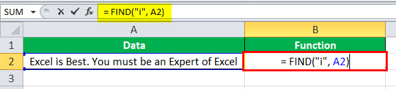
So, the output of the FIND function is 7.

Now, let us pass the previous FIND function as a parameter.

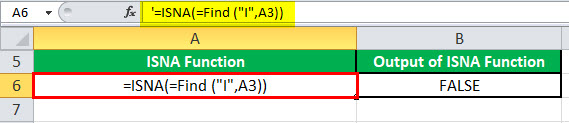
Here, we have used the FIND function in the parameter which returns the output “7”. ISNA function returns “false” because the output of the value parameter is not “#N/A error.”

Example #2

Let us pass “#N/A” directly as a parameter to the ISNA formula in Excel.

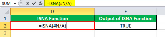
On directly passing “#N/A” as a parameter to the ISNA function, it returns the value “true.” This proves that ISNA detects “#N/A error” present in any cell.

Example #3

Let us pass “#VALUE!” as a parameter to the ISNA formula in Excel.

The “#VALUE!” parameter is also a data missing error. ISNA returns the value “false” because it does not detect any error other than “#N/A error.”

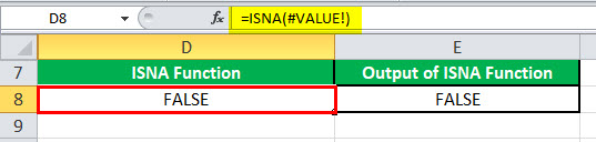
Example #4

In this example, we use the lookup function as a parameter of the ISNA function.

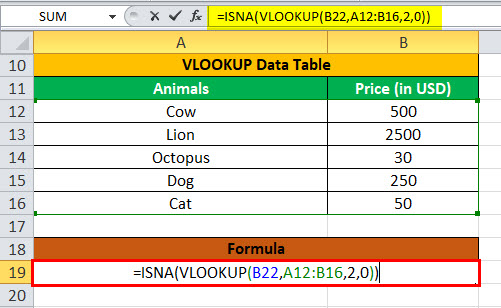
Here, the output that we get is “true.”

Frequently Asked Questions

It helps the Excel user in the following ways:

– It detects “#N/A errors.”
– It helps handle “#N/A errors” by returning a particular value, reference, message or formula.
– It helps replace the “#N/A error” with a text of your choice when combined with VLOOKUP and IF function.
– It finds whether a certain value exists in a column or not when combined with the MATCH function MATCH Function The MATCH function looks for a specific value and returns its relative position in a given range of cells. The output is the first position found for the given value. Being a lookup and reference function, it works for both an exact and approximate match. For example, if the range A11:A15 consists of the numbers 2, 9, 8, 14, 32, the formula “MATCH(8,A11:A15,0)” returns 3. This is because the number 8 is at the third position. read more .
– It facilitates comparison between two columns when combined with the MATCH function.
– It helps analyze results, especially when working with groups of formulas.

The syntax for the ISNA function with VLOOKUP is “=ISNA(VLOOKUP(Argument)).” The VLOOKUP returns “#N/A error” when it is unable to find the value it was looking for. For example, while searching for item X in the lookup table Lookup Table Lookup tables are simply named tables that are used in combination with the VLOOKUP function to find any data in a large data set. We can select the table and name it, and then type the table’s name instead of the reference to look up the value. read more that does not exist, the VLOOKUP will return “#N/A error.”

The ISNA function is combined with VLOOKUP to find out whether the “#N/A error” exists in the data source or not. The IF-ISNA combination can be used with VLOOKUP to return a customized text in place of the “#N/A error.”

The opposite of the ISNA function is “NOT(ISNA(yourformula)).”

If “yourformula” gives “#N/A error,” the ISNA function will return the value “true.” If “yourformula” has no errors, the ISNA function will return the value “false.”

Key Takeaways

The ISNA function is an error handling function in Excel that helps to identify “#N/A error” in a cell.
The ISNA function, used as a worksheet function, has only one parameter.
The value parameter can be another function, formula, cell, or value that needs to be tested.
It returns a Boolean value (true or false).
The value “true” is returned if “#N/A error” is found and “false” is returned if “#N/A error” is not found.

Excel ISNA Function – How To Use

In this tutorial we will show you how the ISNA function works, its synergy effects with other functions, and where it stands against similar error handling functions.

Table of Contents

Syntax

The syntax of the ISNA function is as follows:

Arguments:

value – The value or expression to be tested for #N/A error.

Important Characteristics of ISNA Function in Excel

The ISNA function only deals with #N/A errors
When the function comes across an #N/A error it returns TRUE otherwise it returns FALSE
ISNA is generally used along with the IF function to handle #N/A errors
If the formula has any typos or misspelling, the function returns a #NAME?

Examples of ISNA Function

Now would be a good time to look into some examples to understand the ISNA function.

Example 1 – Simple ISNA function

Let’s take a look at ISNA in its simplest form.

We are checking column A for #N/A errors using the ISNA function in its simplest form:

This is a very basic application of the ISNA function. Let’s move onto more practical examples.

Example 2 – ISNA function with VLOOKUP function

For example, we have a list of dry cake mixes used for baking and their prices.

We are trying to find the prices of a chocolate cake mix and a marble cake mix. Let’s use the VLOOKUP function to find them:

The list of cake mixes doesn’t have «Marble cake» which is why VLOOKUP has returned an «#N/A» error.

Let’s have a look at the results after adding the ISNA function.

We have added the ISNA function to the VLOOKUP function:

All this is doing right now is telling us whether there was an #N/A error while finding the mentioned cake mixes or not.

Was there a ‘not available’ error finding «Chocolate cake» mix? – FALSE. Chocolate cake mix is present in our dataset.

Was there a ‘not available’ error finding «Marble cake» mix? – TRUE. Marble cake mix is not present in our dataset.

Our objective here is to find the prices of the cake mixes which the ISNA function isn’t doing alone. We will have to add the IF function to get the desired results. Let us do that for you.

We have nested the ISNA and VLOOKUP functions in the IF function like so:

This formula works as follows:

VLOOKUP is told to find the data mentioned in cell «E6» which is «Chocolate cake». The table given to VLOOKUP for searching is within the cell range «B2:C11»; VLOOKUP must find «E6» in the 1 st column (column B) of the given table and return the corresponding value from the 2 nd column (column C). «0» indicates that VLOOKUP must find an exact match.

Since «Chocolate cake» is enlisted in the range of cake mixes, VLOOKUP finds it, picks up the corresponding price from the 2 nd column, and returns the value «$3.21».

ISNA vs IFNA

Let us show you how the same outcome can be easily achieved by the IFNA function.

Take note that we have attained the exact same results as in the previous example by lesser work using the formula:

Since «Chocolate cake» was available in our set of data, the VLOOKUP function did its work and returned the value «$3.21». No work for IFNA here.

That was fairly uncomplicated compared to using IF, ISNA, and VLOOKUP functions together.

How to Choose Between ISNA & IFNA

ISNA vs ISERROR

Let’s refer to the previous example and see how this applies.

This doesn’t truly reflect the scenario since the chocolate cake mix and its price is listed in the table. Let’s see what happens when we try to pass the same error through the ISNA function.

Quite useful, ISERROR best serves the need to cover up more errors, affirming whether there are any errors or not.

How to Choose Between ISNA & ISERROR

In most cases, it would be more prudent to use the ISNA function as it would display other errors indicating the relevant issue with the data or formula.

ISNA vs ISERR

How to Choose Between ISNA & ISERR

That’s all ISNA has to say about itself but we still have a little riddle for you:

What kind of career would a spider excel in?

See you with another chip from the Excel block!

Источник

I often need a formula to not return an error value (e.g., «#NA») because it throws off my formulas and pivot tables, so I often find myself throwing an «IF(ISNA» into my formulas to return a custom value or to do another formula in the case of an error otherwise being returned.

But when I have a lot of conditions, this «ISNA» logic gets long and complex so I’d rather use the inverse: «IFNotISNA» a/k/a «IfTrue». Does such an inverse to ISNA exist?

Example: I want to look something up, but if an error is returned I want to look elsewhere — below is how I write these things now (using «IF(ISNA»‘s). This is fine for a few conditionals, but when I want to add a bunch of error-conditional stuff using the «IF(ISNA» the formula gets really clunky and hard to follow.

If(ISNA(Vlookup(Sheet1!A1,Sheet2!X1:Z99,2,false)),Vlookup(Sheet1!A1,Sheet3!X1:Z99,2,false),Vlookup(Sheet1!A1,Sheet2!X1:Z99,2,false)

Thanks!
Jeff

Lock one reference in a formula

Need 1 part of a formula to always point to the same range? use $ signs: $V$2:$Z$99 will always point to V2:Z99, even after copying

You can use:

=IF(NOT(ISNA(YourFormula)),YourFormula,»»)

Within an IF if you want a True returned for a non-ISNA result you could use the following construct:

=IF(1-ISNA(term),Value If Not ISNA, Value if ISNA)

This works because if ISNA() returns True then 1-True = 0 (ie False argument returned), else 1-False=0 (True argument returned).

Thanks so much for the quick help guys! The quick solutions found on this forum never ceases to surprise me!

«If(Not» opens up a lot of doors for me!

Thanks!
Jeff

I often need a formula to not return an error value (e.g., «#NA») because it throws off my formulas and pivot tables, so I often find myself throwing an «IF(ISNA» into my formulas to return a custom value or to do another formula in the case of an error otherwise being returned.

But when I have a lot of conditions, this «ISNA» logic gets long and complex so I’d rather use the inverse: «IFNotISNA» a/k/a «IfTrue». Does such an inverse to ISNA exist?

Example: I want to look something up, but if an error is returned I want to look elsewhere — below is how I write these things now (using «IF(ISNA»‘s). This is fine for a few conditionals, but when I want to add a bunch of error-conditional stuff using the «IF(ISNA» the formula gets really clunky and hard to follow.

If(ISNA(Vlookup(Sheet1!A1,Sheet2!X1:Z99,2,false)),Vlookup(Sheet1!A1,Sheet3!X1:Z99,2,false),Vlookup(Sheet1!A1,Sheet2!X1:Z99,2,false)

Thanks!
Jeff

Another way…

If your lookup formula returns TEXT:

=IF(ISTEXT(your_formula)…

If your lookup formula returns NUMBERS:

=IF(COUNT(your_formula)…

If your lookup formula could return either text or numbers:

=IF(NOT(ISNA(your_formula))…

Источник

No.	IFERROR formula
1	`=IFERROR(G12/F12,"Total Sales are $ 0")`
2	`=IFERROR(G13/F13,"Total Sales are $ 0")`
3	`=IFERROR(G14/F14,"Total Sales are $ 0")`
4	`=IFERROR(G15/F15,"Total Sales are $ 0")`
5	`=IFERROR(G16/F16,"Total Sales are $ 0")`

Description

Syntax

Remarks

Examples

Example 1

Need more help?

Return value

Usage notes

Examples

Return #N/A

Count #N/A errors

Notes

Related Excel Tutorials

IFERROR formula

IFERROR process

IFERROR formula explanation

Item: IFERROR

Item: Value

Item: ValueIfError

IFERROR formula example

Effects of using IFERROR formula example

#2: IFERROR then 0

IFERROR then 0 formula

IFERROR then 0 process

IFERROR then 0 formula explanation

Item: IFERROR

Item: Value

Item: 0

IFERROR then 0 formula example

Effects of using IFERROR then 0 formula example

#3: IFERROR then blank

IFERROR then blank formula

IFERROR then blank process

IFERROR then blank formula explanation

Item: IFERROR

Item: Value

Item: “”

IFERROR then blank formula example

Effects of using IFERROR then blank formula example

#4: IFERROR VLOOKUP

IFERROR VLOOKUP formula

IFERROR VLOOKUP process

IFERROR VLOOKUP formula explanation

Formula #1: VLOOKUP(LookupValue,LookupTable,ColumnIndex,RangeLookup)

Item: VLOOKUP

Item: LookupValue

Item: LookupTable

Item: ColumnIndex

Item: RangeLookup

Formula #2: IFERROR(VLOOKUP(…),ValueIfError)

Item: IFERROR

Item: VLOOKUP(…)

Item: ValueIfError

IFERROR VLOOKUP formula example

Effects of using IFERROR VLOOKUP formula example

#5: ISERROR

ISERROR formula

ISERROR process

ISERROR formula explanation

Item: ISERROR

Item: Value

ISERROR formula example

Effects of using ISERROR formula example

#6: IF ISERROR

IF ISERROR formula

IF ISERROR process

IF ISERROR formula explanation

Formula #1: ISERROR(Value)

Item: ISERROR

Item: Value

Formula #2: IF(ISERROR(…),ValueIfError,Value)

Item: IF

Item: ISERROR(…)

Item: ValueIfError

Item: Value

IF ISERROR formula example

Effects of using IF ISERROR formula example

#7: IF ISERROR VLOOKUP

IF ISERROR VLOOKUP formula

IF ISERROR VLOOKUP process