
Excel for Microsoft 365 Excel for Microsoft 365 for Mac Excel for the web Excel 2021 Excel 2021 for Mac Excel 2019 Excel 2019 for Mac Excel 2016 Excel 2016 for Mac Excel 2013 Excel Web App Excel 2010 Excel 2007 Excel for Mac 2011 Excel Starter 2010 More…Less
You can use the IFERROR function to trap and handle errors in a formula. IFERROR returns a value you specify if a formula evaluates to an error; otherwise, it returns the result of the formula.
Syntax
IFERROR(value, value_if_error)
The IFERROR function syntax has the following arguments:
-
value Required. The argument that is checked for an error.
-
value_if_error Required. The value to return if the formula evaluates to an error. The following error types are evaluated: #N/A, #VALUE!, #REF!, #DIV/0!, #NUM!, #NAME?, or #NULL!.
Remarks
-
If value or value_if_error is an empty cell, IFERROR treats it as an empty string value («»).
-
If value is an array formula, IFERROR returns an array of results for each cell in the range specified in value. See the second example below.
Examples
Copy the example data in the following table, and paste it in cell A1 of a new Excel worksheet. For formulas to show results, select them, press F2, and then press Enter.
|
Quota |
Units Sold |
|
|---|---|---|
|
210 |
35 |
|
|
55 |
0 |
|
|
23 |
||
|
Formula |
Description |
Result |
|
=IFERROR(A2/B2, «Error in calculation») |
Checks for an error in the formula in the first argument (divide 210 by 35), finds no error, and then returns the results of the formula |
6 |
|
=IFERROR(A3/B3, «Error in calculation») |
Checks for an error in the formula in the first argument (divide 55 by 0), finds a division by 0 error, and then returns value_if_error |
Error in calculation |
|
=IFERROR(A4/B4, «Error in calculation») |
Checks for an error in the formula in the first argument (divide «» by 23), finds no error, and then returns the results of the formula. |
0 |
Example 2
|
Quota |
Units Sold |
Ratio |
|---|---|---|
|
210 |
35 |
6 |
|
55 |
0 |
Error in calculation |
|
23 |
0 |
|
|
Formula |
Description |
Result |
|
=C2 |
Checks for an error in the formula in the first argument in the first element of the array (A2/B2 or divide 210 by 35), finds no error, and then returns the result of the formula |
6 |
|
=C3 |
Checks for an error in the formula in the first argument in the second element of the array (A3/B3 or divide 55 by 0), finds a division by 0 error, and then returns value_if_error |
Error in calculation |
|
=C4 |
Checks for an error in the formula in the first argument in the third element of the array (A4/B4 or divide «» by 23), finds no error, and then returns the result of the formula |
0 |
|
Note: If you have a current version of Microsoft 365, then you can input the formula in the top-left-cell of the output range, then press ENTER to confirm the formula as a dynamic array formula. Otherwise, the formula must be entered as a legacy array formula by first selecting the output range, input the formula in the top-left-cell of the output range, then press CTRL+SHIFT+ENTER to confirm it. Excel inserts curly brackets at the beginning and end of the formula for you. For more information on array formulas, see Guidelines and examples of array formulas. |
Need more help?
You can always ask an expert in the Excel Tech Community or get support in the Answers community.
Need more help?
Want more options?
Explore subscription benefits, browse training courses, learn how to secure your device, and more.
Communities help you ask and answer questions, give feedback, and hear from experts with rich knowledge.
Return value
The value you specify for error conditions.
Usage notes
The IFERROR function is used to catch errors and return a more friendly result or message when an error is detected. When a formula returns a normal result, the IFERROR function returns that result. When a formula returns an error, IFERROR returns an alternative result. IFERROR is an elegant way to trap and manage errors. The IFERROR function is a modern alternative to the ISERROR function.
Use the IFERROR function to trap and handle errors produced by other formulas or functions. IFERROR checks for the following errors: #N/A, #VALUE!, #REF!, #DIV/0!, #NUM!, #NAME?, or #NULL!.
Example #1
In the example shown, the formula in E5 copied down is:
=IFERROR(C5/D5,0)
This formula catches the #DIV/0! error that occurs when Qty is empty or zero, and replaces it with zero.
Example #2
For example, if A1 contains 10, B1 is blank, and C1 contains the formula =A1/B1, the following formula will catch the #DIV/0! error that results from dividing A1 by B1:
=IFERROR (A1/B1,"Please enter a value in B1")
As long as B1 is empty, C1 will display the message «Please enter a value in B1» if B1 is blank or zero. When a number is entered in B1, the formula will return the result of A1/B1.
Example #3
You can also use the IFERROR function to catch the #N/A error thrown by VLOOKUP when a lookup value isn’t found. The syntax looks like this:
=IFERROR(VLOOKUP(value,data,column,0),"Not found")
In this example, when VLOOKUP returns a result, IFERROR functions that result. If VLOOKUP returns #N/A error because a lookup value isn’t found, IFERROR returns «Not Found».
IFERROR or IFNA?
The IFERROR function is a useful function, but it is a blunt instrument since it will trap many kinds of errors. For example, if there’s a typo in a formula, Excel may return the #NAME? error, but IFERROR will suppress the error and return the alternative result. This can obscure an important problem. In many cases, it makes more sense to use the IFNA function, which only traps the #N/A error.
Other error functions
Excel provides a number of error-related functions, each with a different behavior:
- The ISERR function returns TRUE for any error type except the #N/A error.
- The ISERROR function returns TRUE for any error.
- The ISNA function returns TRUE for #N/A errors only.
- The ERROR.TYPE function returns the numeric code for a given error.
- The IFERROR function traps errors and provides an alternative result.
- The IFNA function traps #N/A errors and provides an alternative result.
Notes
- If value is empty, it is evaluated as an empty string («») and not an error.
- If value_if_error is supplied as an empty string («»), no message is displayed when an error is detected.
- In Excel 2013+, you can use the IFNA function to trap and handle #N/A errors specifically.
Функция IFERROR (ЕСЛИОШИБКА) в Excel лучше всего подходит для обработки случаев, когда формулы возвращают ошибку. Используя эту функцию, вы можете указать, какое значение функция должна возвращать вместо ошибки. Если функция в ячейке не возвращает ошибку, то возвращается её собственный результат.
Содержание
- Видеоурок
- Что возвращает функция
- Синтаксис
- Аргументы функции
- Дополнительная информация
- Примеры использования функции IFERROR (ЕСЛИОШИБКА) в Excel
- Пример 1. Заменяем ошибки в ячейке на пустые значения
- Пример 2. Заменяем значения без данных при использовании функции VLOOKUP (ВПР) на “Не найдено”
- Пример 3. Возвращаем значение “0” вместо ошибок формулы
Видеоурок
Что возвращает функция
Указанное вами значение, в случае если в ячейке есть ошибка.
Синтаксис
=IFERROR(value, value_if_error) — английская версия
=ЕСЛИОШИБКА(значение;значение_если_ошибка) — русская версия
Аргументы функции
- value (значение) — это аргумент, который проверяет, есть ли в ячейке ошибка. Обычно, ошибкой может быть результат какого либо вычисления;
- value_if_error (значение_если_ошибка) — это аргумент, который заменяет ошибку в ячейке (в случае её наличия) на указанное вами значение. Ошибки могут выглядеть так: #N/A, #REF!, #DIV/0!, #VALUE!, #NUM!, #NAME?, #NULL! (английская версия Excel) или #ЗНАЧ!, #ДЕЛ/0, #ИМЯ?, #Н/Д, #ССЫЛКА!, #ЧИСЛО!, #ПУСТО! (русская версия Excel).
Дополнительная информация
- Если вы используете кавычки («») в качестве аргумента value_if_error (значение_если_ошибка), ячейка ничего не отображает в случае ошибки.
- Если аргумент value (значение) или value_if_error (значение_если_ошибка) ссылается на пустую ячейку, она рассматривается как пустая.
Примеры использования функции IFERROR (ЕСЛИОШИБКА) в Excel
Пример 1. Заменяем ошибки в ячейке на пустые значения
Если вы используете функции, которые могут возвращать ошибку, вы можете заключить ее в функцию и указать пустое значение, возвращаемое в случае ошибки.
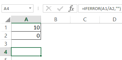
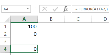
В примере, показанном ниже, результатом ячейки D4 является # DIV/0!.

Для того, чтобы убрать информацию об ошибке в ячейке используйте эту формулу:
=IFERROR(A1/A2,””) — английская версия
=ЕСЛИОШИБКА(A1/A2;»») — русская версия
В данном случае функция проверит, выдает ли формула в ячейке ошибку, и, при её наличии, выдаст пустой результат.
В качестве результата формулы, исправляющей ошибки, вы можете указать любой текст или значение, например, с помощью следующей формулы:
Больше лайфхаков в нашем Telegram Подписаться
=IFERROR(A1/A2,”Error”) — английская версия
=ЕСЛИОШИБКА(A1/A2;»») — русская версия
Если вы пользуетесь версией Excel 2003 или ниже, вы не найдете функцию IFERROR (ЕСЛИОШИБКА). Вместо нее вы можете использовать обычную функцию IF или ISERROR.
Пример 2. Заменяем значения без данных при использовании функции VLOOKUP (ВПР) на “Не найдено”
Когда мы используем функцию VLOOKUP (ВПР), часто сталкиваемся с тем, что при отсутствии данных по каким либо значениям, формула выдает ошибку “#N/A”.
На примере ниже, мы хотим с помощью функции VLOOKUP (ВПР) для выбранных студентов подставить данные из результатов экзамена.
На примере выше, в списке студентов с результатами экзамена нет данных по имени Иван, в результате, при использовании функции VLOOKUP (ВПР), формула нам выдает ошибку.
Как раз в этом случае мы можем воспользоваться функцией IFERROR (ЕСЛИОШИБКА), для того, чтобы результат вычислений выглядел корректно, без ошибок. Добиться этого мы можем с помощью формулы:
=IFERROR(VLOOKUP(D2,$A$2:$B$12,2,0),”Не найдено”) — английская версия
=ЕСЛИОШИБКА(ВПР(D2;$A$2:$B$12;2;0);»Не найдено») — русская версия
Пример 3. Возвращаем значение “0” вместо ошибок формулы
Если у вас нет конкретного значения, которое вы бы хотели использовать для замены ошибок — оставляйте аргумент функции value_if_error (значение_если_ошибка) пустым, как показано на примере ниже и в случае наличия ошибки, функция будет выдавать “0”:
Things will not always be the way we want them to be. The unexpected can happen. For example, let’s say you have to divide numbers. Trying to divide any number by zero (0) gives an error. Logical functions come in handy such cases. In this tutorial, we are going to cover the following topics.
In this tutorial, we are going to cover the following topics.
- What is a Logical Function?
- IF function example
- Excel Logic functions explained
- Nested IF functions
What is a Logical Function?
It is a feature that allows us to introduce decision-making when executing formulas and functions. Functions are used to;
- Check if a condition is true or false
- Combine multiple conditions together
What is a condition and why does it matter?
A condition is an expression that either evaluates to true or false. The expression could be a function that determines if the value entered in a cell is of numeric or text data type, if a value is greater than, equal to or less than a specified value, etc.
IF Function example
We will work with the home supplies budget from this tutorial. We will use the IF function to determine if an item is expensive or not. We will assume that items with a value greater than 6,000 are expensive. Those that are less than 6,000 are less expensive. The following image shows us the dataset that we will work with.
 and conditions in Excel")
- Put the cursor focus in cell F4
- Enter the following formula that uses the IF function
=IF(E4<6000,”Yes”,”No”)
HERE,
- “=IF(…)” calls the IF functions
- “E4<6000” is the condition that the IF function evaluates. It checks the value of cell address E4 (subtotal) is less than 6,000
- “Yes” this is the value that the function will display if the value of E4 is less than 6,000
-
“No” this is the value that the function will display if the value of E4 is greater than 6,000
When you are done press the enter key
You will get the following results
 and conditions in Excel")
Excel Logic functions explained
The following table shows all of the logical functions in Excel
| S/N | FUNCTION | CATEGORY | DESCRIPTION | USAGE |
|---|---|---|---|---|
| 01 | AND | Logical | Checks multiple conditions and returns true if they all the conditions evaluate to true. | =AND(1 > 0,ISNUMBER(1)) The above function returns TRUE because both Condition is True. |
| 02 | FALSE | Logical | Returns the logical value FALSE. It is used to compare the results of a condition or function that either returns true or false | FALSE() |
| 03 | IF | Logical |
Verifies whether a condition is met or not. If the condition is met, it returns true. If the condition is not met, it returns false. =IF(logical_test,[value_if_true],[value_if_false]) |
=IF(ISNUMBER(22),”Yes”, “No”) 22 is Number so that it return Yes. |
| 04 | IFERROR | Logical | Returns the expression value if no error occurs. If an error occurs, it returns the error value | =IFERROR(5/0,”Divide by zero error”) |
| 05 | IFNA | Logical | Returns value if #N/A error does not occur. If #N/A error occurs, it returns NA value. #N/A error means a value if not available to a formula or function. |
=IFNA(D6*E6,0) N.B the above formula returns zero if both or either D6 or E6 is/are empty |
| 06 | NOT | Logical | Returns true if the condition is false and returns false if condition is true |
=NOT(ISTEXT(0)) N.B. the above function returns true. This is because ISTEXT(0) returns false and NOT function converts false to TRUE |
| 07 | OR | Logical | Used when evaluating multiple conditions. Returns true if any or all of the conditions are true. Returns false if all of the conditions are false |
=OR(D8=”admin”,E8=”cashier”) N.B. the above function returns true if either or both D8 and E8 admin or cashier |
| 08 | TRUE | Logical | Returns the logical value TRUE. It is used to compare the results of a condition or function that either returns true or false | TRUE() |
A nested IF function is an IF function within another IF function. Nested if statements come in handy when we have to work with more than two conditions. Let’s say we want to develop a simple program that checks the day of the week. If the day is Saturday we want to display “party well”, if it’s Sunday we want to display “time to rest”, and if it’s any day from Monday to Friday we want to display, remember to complete your to do list.
A nested if function can help us to implement the above example. The following flowchart shows how the nested IF function will be implemented.
 and conditions in Excel")
The formula for the above flowchart is as follows
=IF(B1=”Sunday”,”time to rest”,IF(B1=”Saturday”,”party well”,”to do list”))
HERE,
- “=IF(….)” is the main if function
- “=IF(…,IF(….))” the second IF function is the nested one. It provides further evaluation if the main IF function returned false.
Practical example
 and conditions in Excel")
Create a new workbook and enter the data as shown below
 and conditions in Excel")
- Enter the following formula
=IF(B1=”Sunday”,”time to rest”,IF(B1=”Saturday”,”party well”,”to do list”))
- Enter Saturday in cell address B1
- You will get the following results
 and conditions in Excel")
Download the Excel file used in Tutorial
Summary
Logical functions are used to introduce decision-making when evaluating formulas and functions in Excel.
What is IF Function in Excel?
IF function in Excel evaluates whether a given condition is met and returns a value depending on whether the result is “true” or “false”. It is a conditional function of Excel, which returns the result based on the fulfillment or non-fulfillment of the given criteria.
For example, the IF formula in Excel can be applied as follows:
“=IF(condition A,“value B”,“value C”)”
The IF excel function returns “value B” if condition A is met and returns “value C” if condition A is not met.
It is often used to make logical interpretations which help in decision-making.
Table of contents
- What is IF Function in Excel?
- Syntax of the IF Excel Function
- How to Use IF Function in Excel?
- Example #1
- Example #2
- Example #3
- Example #4
- Example #5
- Guidelines for the Multiple IF Statements
- Frequently Asked Question
- IF Excel Function Video
- Recommended Articles
Syntax of the IF Excel Function
The syntax of the IF function is shown in the following image:

The IF excel function accepts the following arguments:
- Logical_test: It refers to the condition to be evaluated. The condition can be a value or a logical expression.
- Value_if_true: It is the value returned as a result when the condition is “true”.
- Value_if_false: It is the value returned as a result when the condition is “false”.
In the formula, the “logical_test” is a required argument, whereas the “value_if_true” and “value_if_false” are optional arguments.
The IF formula uses logical operators to evaluate the values in a range of cells. The following table shows the different logical operatorsLogical operators in excel are also known as the comparison operators and they are used to compare two or more values, the return output given by these operators are either true or false, we get true value when the conditions match the criteria and false as a result when the conditions do not match the criteria.read more and their meaning.
| Operator | Meaning |
|---|---|
| = | Equal to |
| > | Greater than |
| >= | Greater than or equal to |
| < | Less than |
| <= | Less than or equal to |
| <> | Not equal to |
How to Use IF Function in Excel?
Let us understand the working of the IF function with the help of the following examples in Excel.
You can download this IF Function Excel Template here – IF Function Excel Template
Example #1
If there is no oxygen on a planet, life is impossible. If oxygen is available on a planet, then life is possible. The following table shows a list of planets in column A and the information on the availability of oxygen in column B. We have to find the planets where life is possible, based on the condition of oxygen availability.

Let us apply the IF formula to cell C2 to find out whether life is possible on the planets listed in the table.
The IF formula is stated as follows:
“=IF(B2=“Yes”, “Life is Possible”, “Life is Not Possible”)
The succeeding image shows the IF formula applied to cell C2.

The subsequent image shows how the IF formula is applied to the range of cells C2:C5.

Drag the cells to view the output of all the planets.

The output in the below worksheet shows life is possible on the planet Earth.
Flow Chart of Generic IF Excel Function

The IF Function Flow Chart for Mars (Example #1)

The flow of IF function flowchart for Jupiter and Venus is the same as the IF function flowchart for Mars (Example #1).
The IF Function Flow Chart for Earth

Hence, the IF excel function allows making logical comparisons between values. The modus operandi of the IF function is stated as: If something is true, then do something; otherwise, do something else.
Example #2
The following table shows a list of years. We want to find out if the given year is a leap year or not.
A leap year has 366 days; the extra day is the 29th of February. The criteria for a leap year are stated as follows:
- The year will be exactly divisible by 4 and not exactly be divisible by 100 or
- The year will be exactly divisible by 400.

In this example, we will use the IF function along with the AND, OR, and MOD functions to find the leap years.
We use the MOD function to find a remainder after a dividend is divided by a divisor.
The AND functionThe AND function in Excel is classified as a logical function; it returns TRUE if the specified conditions are met, otherwise it returns FALSE.read more evaluates both the conditions of the leap years for the value “true”. The OR functionThe OR function in Excel is used to test various conditions, allowing you to compare two values or statements in Excel. If at least one of the arguments or conditions evaluates to TRUE, it will return TRUE. Similarly, if all of the arguments or conditions are FALSE, it will return FASLE.read more evaluates either of the condition for the value “true”.
We will apply the MOD function to the conditions as follows:
If MOD(year,4)=0 and MOD(year,100)<>(is not equal to) 0, then the year is a leap year.
or
If MOD(year,400)=0, then the year is a leap year; otherwise, the year is not a leap year.
The IF formula is stated as follows:
“=IF(OR(AND((MOD(year,4)=0),(MOD(year,100)<>0)),(MOD(year,400)=0)),“Leap Year”, “Not A Leap Year”)”
The argument “year” refers to a reference value.
The following images show the output of the IF formula applied in the range of cells.


The following image shows how the IF formula is applied to the range of cells B2:B18.

The succeeding table shows the years 1960, 2028, and 2148 as leap years and the remaining as non-leap years.

The result of the IF excel formula is displayed for the range of cells B2:B18 in the following image.

Example #3
The succeeding table shows a list of drivers and the directions they undertook to reach the destination. It is preceded by an image of the road intersection explaining the turns taken by the drivers and their destinations. The right turn leads to town B, and the left turn leads to town C. Identify the driver’s destination to town B and town C.
Road Intersection Image


Let us apply the IF excel function to find the destination. Here, the condition is mentioned as follows:
- If the driver turns right, he/she reaches town B.
- If the driver turns left, he/she reaches town C.
We use the following IF formula to find the destination:
“=IF(B2=“Left”, “Town C”, “Town B”)”
The succeeding image shows the output of the IF formula applied to cell C2.

Drag the cells to use the formula in the range C2:C11. Finally, we get the destinations of each driver for their turning movements.
The below image displays the IF formula applied to the range.

The output of the IF formula and the destinations are displayed in the succeeding image.

The result shows that six drivers reached town C, and the remaining four have reached town B.
Example #4
The following table shows a list of items and their inventory levels. We want to check if the specific item is available in the inventory or not using the IF function.

Let us list the name of items in column A and the number of items in column B. The list of data to be validated for the entire items list is shown in the cell E2 of the below image.

We use the Excel IF along with the VLOOKUP functionThe VLOOKUP excel function searches for a particular value and returns a corresponding match based on a unique identifier. A unique identifier is uniquely associated with all the records of the database. For instance, employee ID, student roll number, customer contact number, seller email address, etc., are unique identifiers.
read more to check the availability of the items in the inventory.
The VLOOKUP function looks up the values referring to the number of items, and the IF function will check whether the item number is greater than zero or not.
We will apply the following IF formula in the F2 cell:
“=IF(VLOOKUP(E2,A2:B11,2,0)=0, “Item Not Available”,“Item Available”)”
If the lookup value of an item is equal to 0, then the item is not available; else, the item is available.
The succeeding image shows the result of the IF formula in the cell F2.

Select “bat” in the E2 item cell to know whether the item is available or not in the inventory (as shown in the following image).

Example #5
The following table shows the list of students and their marks. The grade criteria are provided based on the marks obtained by the students. We want to find the grade of each student in the list.

We apply the Nested IF in Excel since we have multiple criteria to find and decide each student’s grade.
The Nesting of IF function uses the IF function inside another IF formula when multiple conditions are to be fulfilled.
The syntax of Nesting of IF function is stated as follows:
“=IF( condition1, value_if_true1, IF( condition2, value_if_true2, value_if_false2 ))”
The succeeding table represents the range of scores and the grades, respectively.

Let us apply the multiple IF conditions with AND function in the below-nested formula to find out the grade of the students:
“=IF((B2>=95),“A”,IF(AND(B2>=85,B2<=94),“B”,IF(AND(B2>=75,B2<=84),“C”,IF(AND(B2>=61,B2<=74),“D”,“F”))))”
The IF function checks the logical condition as shown in the formula below:
“=IF(logical_test, [value_if_true],[value_if_false])”
We will split the above-mentioned nested formula and check the IF statements as shown below:
First Logical Test: B2>=95
If the formula returns,
- Value_if_true, execute: “A” (Grade A) else(comma) enter value_if_false
- Value_if_false, then the formula finds another IF condition and enter IF condition
Second Logical Test: B2>=85(logical expression 1) and B2<=94(logical expression 2)
(We use AND function to check the multiple logical expressions as the two given conditions are to be evaluated for “true.”)
If the formula returns,
- Value_if_true, execute: “B” (Grade B) else(comma) enter value_if_false
- Value_if_false, then the formula finds another IF condition and enter IF condition
Third Logical Test: B2>=75(logical expression 1) and B2<=84(logical expression 2)
(We use AND function to check the multiple logical expressions as the two given conditions are to be evaluated for “true.”)
If the formula returns,
- Value_if_true, execute: “C” (Grade C) else(comma) enter value_if_false
- value_if_false, then the formula finds another IF condition and enter IF condition
Fourth Logical Test: B2>=61(logical expression 1) and B2<=74(logical expression 2)
(We use AND function to check the multiple logical expressions as the two given conditions are to be evaluated for “true.”)
If the formula returns,
- Value_if_true, execute: “D” (Grade D) else(comma) enter value_if_false
- Value_if_false, execute: “F” (Grade F)
- Finally, close the parenthesis.
The below image displays the output of the IF formula applied to the range.

The succeeding image shows the IF nested formula applied to the range.

The grades of the students are listed in the following table.

Guidelines for the Multiple IF Statements
The guidelines for the multiple IF statements are listed as follows:
- Use nested IF function to a limited extent as multiple IF statements require a great deal of thought to be accurate.
- Multiple IF statementsIn Excel, multiple IF conditions are IF statements that are contained within another IF statement. They are used to test multiple conditions at the same time and return distinct values. Additional IF statements can be included in the ‘value if true’ and ‘value if false’ arguments of a standard IF formula.read more require multiple parentheses (), which is often difficult to manage. Excel provides a way to check the color of each opening and closing parenthesis to avoid this situation. The last closing parenthesis color will always be black, denoting the end of the formula statement.
- Whenever we pass a string value for the arguments “value_if_true” and “value_if_false” or test a reference against a string value, enclose the string value in double quotes. Passing a string value without quotes will result in “#NAME?” error.
Frequently Asked Question
1. What is the IF function in Excel?
The Excel IF function is a logical function that checks the given criteria and returns one value for a “true” and another value for a “false” result.
The syntax of the IF function is stated as follows:
“=IF(logical_test, [value_if_true], [value_if_false])”
The arguments are as follows:
1. Logical_test – It refers to a value or condition that is tested.
2. Value_if_true – It is the value returned when the condition logical_test is “true.”
3. Value_if_false – It is the value returned when the condition logical_test is “false.”
The “logical_test” is a required argument, whereas the “value_if_true” and “value_if_false” are optional arguments.
2. How to use the IF Excel function with multiple conditions?
The IF Excel statement for multiple conditions is created by using multiple IF functions in a single formula.
The syntax of IF function with multiple conditions is stated as follows:
“=IF (condition 1_“true”, do something, IF (condition 2_“true”, do something, IF (condition 3_ “true”, do something, else do something)))”
3. How to use the function IFERROR in Excel?
IF Excel Function Video
Recommended Articles
This has been a guide to the IF function in Excel. Here we discuss how to use the IF function along with examples and downloadable templates. You may also look at these useful functions –
- What is the Logical Test in Excel?A logical test in Excel results in an analytical output, either true or false. The equals to operator, “=,” is the most commonly used logical test.read more
- “Not Equal to” in Excel“Not Equal to” argument in excel is inserted with the expression <>. The two brackets posing away from each other command excel of the “Not Equal to” argument, and the user then makes excel checks if two values are not equal to each other.read more
- Data Validation ExcelThe data validation in excel helps control the kind of input entered by a user in the worksheet.read more
Skip to content
В статье описано, как использовать функцию ЕСЛИОШИБКА в Excel для обнаружения ошибок и замены их пустой ячейкой, другим значением или определённым сообщением. Покажем примеры, как использовать функцию ЕСЛИОШИБКА с функциями визуального просмотра и сопоставления индексов, а также как она сравнивается с ЕСЛИ ОШИБКА и ЕСНД.
«Дайте мне точку опоры, и я переверну землю», — сказал однажды Архимед. «Дайте мне формулу, и я заставлю ее вернуть ошибку», — сказал бы пользователь Excel. Здесь мы не будем рассматривать, как получить ошибки в Excel. Мы узнаем, как предотвратить их, чтобы ваши таблицы были чистыми, а формулы — понятными и точными.
Итак, вот о чем мы поговорим:
Что означает функция Excel ЕСЛИОШИБКА
Функция ЕСЛИОШИБКА (IFERROR по-английски) предназначена для обнаружения и устранения ошибок в формулах и вычислениях. Это значит, что функция ЕСЛИОШИБКА должна выполнить определенные действия, если видит какую-либо ошибку. Более конкретно, она проверяет формулу и, если вычисление дает ошибку, то она возвращает какое-то другое значение, которое вы ей укажете. Если же всё хорошо, то просто возвращает результат формулы.
Синтаксис функции Excel ЕСЛИОШИБКА следующий:
ЕСЛИОШИБКА(значение; значение_если_ошибка)
Где:
- Значение (обязательно) — что проверять на наличие ошибок. Это может быть формула, выражение или ссылка на ячейку.
- Значение_если_ошибка (обязательно) — что возвращать при обнаружении ошибки. Это может быть пустая строка (получится пустая ячейка), текстовое сообщение, числовое значение, другая формула или вычисление.
Например, при делении двух столбцов чисел можно получить кучу разных ошибок, если в одном из столбцов есть пустые ячейки, нули или текст.
Рассмотрим простой пример:

Чтобы этого не произошло, используйте формулу ЕСЛИОШИБКА, чтобы перехватывать и обрабатывать их нужным вам образом.
Если ошибка, то пусто
Укажите пустую строку (“”) в аргументе значение_если_ошибка, чтобы вернуть пустую ячейку, если обнаружена ошибка:
=ЕСЛИОШИБКА(A4/B4; «»)
Вернемся к нашему примеру и используем ЕСЛИОШИБКА:

Как видите по сравнению с первым скриншотом, вместо стандартных сообщений мы видим просто пустые ячейки.
Если ошибка, то показать сообщение
Вы также можете отобразить собственное сообщение вместо стандартного обозначения ошибок Excel:
=ЕСЛИОШИБКА(A4/B4; «Ошибка в вычислениях»)
Перед вами – третий вариант нашей небольшой таблицы.

5 фактов, которые нужно знать о функции ЕСЛИОШИБКА в Excel
- ЕСЛИОШИБКА в Excel обрабатывает все типы ошибок, включая #ДЕЛ/0!, #Н/Д, #ИМЯ?, #NULL!, #ЧИСЛО!, #ССЫЛКА! и #ЗНАЧ!.
- В зависимости от содержимого аргумента значение_если_ошибка функция может заменить ошибки вашим текстовым сообщением, числом, датой или логическим значением, результатом другой формулы или пустой строкой (пустой ячейкой).
- Если аргумент значение является пустой ячейкой, он обрабатывается как пустая строка (»’), но не как ошибка.
- ЕСЛИОШИБКА появилась в Excel 2007 и доступна во всех последующих версиях Excel 2010, Excel 2013, Excel 2016, Excel 2019, Excel 2021 и Excel 365.
- Чтобы перехватывать ошибки в Excel 2003 и более ранних версиях, используйте функцию ЕОШИБКА в сочетании с функцией ЕСЛИ, например как показано ниже:
=ЕСЛИ(ЕОШИБКА(A4/B4);»Ошибка в вычислениях»;A4/B4)
Далее вы увидите, как можно использовать ЕСЛИОШИБКА в Excel в сочетании с другими функциями для выполнения более сложных задач.
ЕСЛИОШИБКА с функцией ВПР
Часто встречающаяся задача в Excel – поиск нужного значения в таблице в соответствии с определёнными критериями. И не всегда этот поиск бывает успешным. Одним из наиболее распространенных применений функции ЕСЛИОШИБКА является сообщение пользователям, что искомое значение не найдено в базе данных. Для этого вы заключаете формулу ВПР в функцию ЕСЛИОШИБКА примерно следующим образом:
ЕСЛИОШИБКА(ВПР( … );»Не найдено»)
Если искомое значение отсутствует в таблице, которую вы просматриваете, обычная формула ВПР вернет ошибку #Н/Д:

Для лучшего понимания таблицы и улучшения ее внешнего вида, заключите функцию ВПР в ЕСЛИОШИБКА и покажите более понятное для пользователя сообщение:
=ЕСЛИОШИБКА(ВПР(D3; $A$3:$B$5; 2;ЛОЖЬ); «Не найдено»)
На скриншоте ниже показан пример ЕСЛИОШИБКА вместе с ВПР в Excel:

Если вы хотите перехватывать только #Н/Д, но не все подряд ошибки, используйте функцию ЕНД вместо ЕСЛИОШИБКА. Она просто возвращает ИСТИНА или ЛОЖЬ в зависимости от появления ошибки #Н/Д. Поэтому нам здесь еще понадобится функция ЕСЛИ, чтобы обработать эти логические значения:
=ЕСЛИ(ЕНД(ВПР(D3; $A$3:$B$5; 2;ЛОЖЬ)); «Не найдено»;ВПР(D3; $A$3:$B$5; 2;ЛОЖЬ))
Дополнительные примеры формул Excel ЕСЛИОШИБКА ВПР можно также найти в нашей статье Как убрать сообщение #Н/Д в ВПР?
Вложенные функции ЕСЛИОШИБКА для выполнения последовательных ВПР
В ситуациях, когда вам нужно выполнить несколько операций ВПР в зависимости от того, была ли предыдущая ВПР успешной или неудачной, вы можете вложить две или более функции ЕСЛИОШИБКА одну в другую.
Предположим, у вас есть несколько отчетов о продажах из региональных отделений вашей компании, и вы хотите получить сумму по определенному идентификатору заказа. С ячейкой В9 в качестве критерия поиска (номер заказа) и тремя небольшими таблицами поиска (таблица 1, 2 и 3), формула выглядит следующим образом:
=ЕСЛИОШИБКА(ВПР(B9;A3:B6;2;0);ЕСЛИОШИБКА(ВПР(B9;D3:E6;2;0);ЕСЛИОШИБКА(ВПР(B9;G3:H6;2;0);»Не найден»)))
Результат будет выглядеть примерно так, как на рисунке ниже:

То есть, если поиск завершился неудачей (то есть, ошибкой) первой таблице, начинаем искать во второй, и так далее. Если нигде ничего не нашли, получим сообщение «Не найден».
ЕСЛИОШИБКА в формулах массива
Как вы, наверное, знаете, формулы массива в Excel предназначены для выполнения нескольких вычислений внутри одной формулы. Если вы в аргументе значение функции ЕСЛИОШИБКА укажете формулу или выражение, которое возвращает массив, она также обработает и вернет массив значений для каждой ячейки в указанном диапазоне. Пример ниже поможет пояснить это.
Допустим, у вас есть Сумма в столбце B и Цена в столбце C, и вы хотите вычислить Количество. Это можно сделать с помощью следующей формулы массива, которая делит каждую ячейку в диапазоне B2:B4 на соответствующую ячейку в диапазоне C2:C4, а затем суммирует результаты:
=СУММ(($B$2:$B$4/$C$2:$C$4))
Формула работает нормально, пока в диапазоне делителей нет нулей или пустых ячеек. Если есть хотя бы одно значение 0 или пустая строка, то возвращается ошибка: #ДЕЛ/0! Из-за одной некорректной позиции мы не можем получить итоговый результат.

Чтобы исправить эту ситуацию, просто вложите деление внутрь формулы ЕСЛИОШИБКА:
=СУММ(ЕСЛИОШИБКА($B$2:$B$4/$C$2:$C$4;0))

Что делает эта формула? Делит значение в столбце B на значение в столбце C в каждой строке (3500/100, 2000/50 и 0/0) и возвращает массив результатов {35; 40; #ДЕЛ/0!}. Функция ЕСЛИОШИБКА перехватывает все ошибки #ДЕЛ/0! и заменяет их нулями. Затем функция СУММ суммирует значения в итоговом массиве {35; 40; 0} и выводит окончательный результат (35+40=75).
Примечание. Помните, что ввод формулы массива должен быть завершен нажатием комбинации Ctrl + Shift + Enter (если у вас не Office365 или Excel2021 – они понимают формулы массива без дополнительных телодвижений).
ЕСЛИОШИБКА или ЕСЛИ + ЕОШИБКА?
Теперь, когда вы знаете, как использовать функцию ЕСЛИОШИБКА в Excel, вы можете удивиться, почему некоторые люди все еще склоняются к использованию комбинации ЕСЛИ + ЕОШИБКА. Есть ли у этого старого метода преимущества по сравнению с ЕСЛИОШИБКА?
В старые недобрые времена Excel 2003 и более ранних версий, когда ЕСЛИОШИБКА не существовало, совместное использование ЕСЛИ и ЕОШИБКА было единственным возможным способом перехвата ошибок. Это просто немного более сложный способ достижения того же результата.
Например, чтобы отловить ошибки ВПР, вы можете использовать любую из приведенных ниже формул.
В Excel 2007 — Excel 2016:
ЕСЛИОШИБКА(ВПР( … ); «Не найдено»)
Во всех версиях Excel:
ЕСЛИ(ЕОШИБКА(ВПР(…)); «Не найдено»; ВПР(…))
Обратите внимание, что в формуле ЕСЛИ ЕОШИБКА ВПР вам нужно дважды выполнить ВПР. Чтобы лучше понять, расшифруем: если ВПР приводит к ошибке, вернуть «Не найдено», в противном случае вывести результат ВПР.
А вот простой пример формулы Excel ЕСЛИ ЕОШИБКА ВПР:
=ЕСЛИ(ЕОШИБКА(ВПР(D2; A2:B5;2;ЛОЖЬ)); «Не найдено»; ВПР(D2; A2:B5;2;ЛОЖЬ ))

ЕСЛИОШИБКА против ЕСНД
Представленная в Excel 2013, ЕСНД (IFNA в английской версии) — это еще одна функция для проверки формулы на наличие ошибок. Его синтаксис похож на синтаксис ЕСЛИОШИБКА:
ЕСНД(значение; значение_если_НД)
Чем ЕСНД отличается от ЕСЛИОШИБКА? Функция ЕСНД перехватывает только ошибки #Н/Д, тогда как ЕСЛИОШИБКА обрабатывает все типы ошибок.
В каких ситуациях вы можете использовать ЕСНД? Когда нецелесообразно скрывать все ошибки. Например, при работе с важными данными вы можете захотеть получать предупреждения о возможных ошибках в вашем наборе данных (случайном делении на ноль и т.п.), а стандартные сообщения об ошибках Excel с символом «#» могут быть яркими визуальными индикаторами проблем.
Давайте посмотрим, как можно создать формулу, отображающую сообщение «Не найдено» вместо ошибки «Н/Д», которая появляется, когда искомое значение отсутствует в наборе данных, но при этом вы будете видеть все другие ошибки Excel.
Предположим, вы хотите получить Количество из таблицы поиска в таблицу с результатами, как показано на рисунке ниже. Проще всего было бы использовать ЕСЛИОШИБКА с ВПР. Таблица приобрела бы красивый вид, но при этом за надписью «Не найдено» были бы скрыты не только ошибки поиска, но и все другие ошибки. И мы не заметили бы, что в исходной таблице поиска у нас есть ошибка деления на ноль, так как не заполнена цена персиков. Поэтому более разумно использовать ЕСНД, чтобы с ее помощью обработать только ошибки поиска:
=ЕСНД(ВПР(F3; $A$3:$D$6; 4;ЛОЖЬ); «Не найдено»)

Или подойдет комбинация ЕСЛИ ЕНД для старых версий Excel:
=ЕСЛИ(ЕНД(ВПР(F3; $A$3:$D$6; 4;ЛОЖЬ));»Не найдено»; ВПР(F3; $A$3:$D$6; 4;ЛОЖЬ))
Как видите, формула ЕСНД с ВПР возвращает «Не найдено» только для товара, которого нет в таблице поиска (Сливы). Для персиков она показывает #ДЕЛ/0! что указывает на то, что наша таблица поиска содержит ошибку деления на ноль.
Рекомендации по использованию ЕСЛИОШИБКА в Excel
Итак, вы уже знаете, что функция ЕСЛИОШИБКА — это самый простой способ отлавливать ошибки в Excel и маскировать их пустыми ячейками, нулевыми значениями или собственными сообщениями. Однако это не означает, что вы должны обернуть каждую формулу в функцию обработки ошибок.
Эти простые рекомендации могут помочь вам сохранить баланс.
- Не ловите ошибки без весомой на то причины.
- Оберните в ЕСЛИОШИБКА только ту часть формулы, где по вашему мнению могут возникнуть проблемы.
- Чтобы обрабатывать только определенные ошибки, используйте другую функцию обработки ошибок с меньшей областью действия:
- ЕСНД или ЕСЛИ ЕНД для обнаружения только ошибок #H/Д.
- ЕОШ для обнаружения всех ошибок, кроме #Н/Д.
Мы постарались рассказать, как можно использовать функцию ЕСЛИОШИБКА в Excel. Примеры перехвата и обработки ошибок могут быть полезны и для «чайников», и для более опытных пользователей.
Также рекомендуем:
When you work with data and formulas in Excel, you’re bound to encounter errors.
To handle errors, Excel has provided a useful function – the IFERROR function.
Before we get into the mechanics of using the IFERROR function in Excel, let’s first go through the different kinds of errors you can encounter when working with formulas.
Types of Errors in Excel
Knowing the errors in Excel will better equip you to identify the possible reason and the best way to handle these.
Below are the types of errors you might find in Excel.
#N/A Error
This is called the ‘Value Not Available’ error.
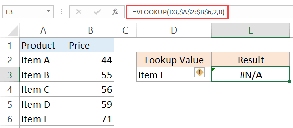
You will see this when you use a lookup formula and it can’t find the value (hence Not Available).
Below is an example where I use the VLOOKUP formula to find the price of an item, but it returns an error when it can’t find that item in the table array.
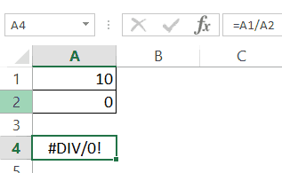
#DIV/0! Error
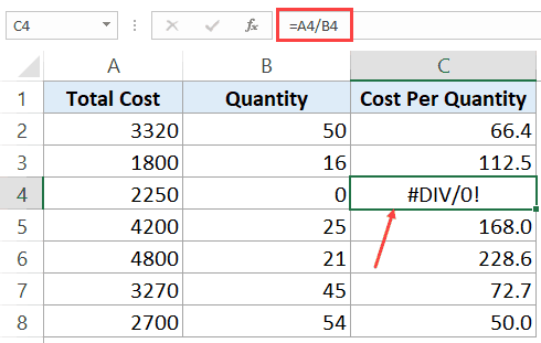
You’re likely to see this error when a number is divided by 0.
This is called the division error. In the below example, it gives a #DIV/0! error as the quantity value (the divisor in the formula) is 0.
#VALUE! Error
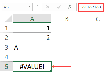
The value error occurs when you use an incorrect data type in a formula.
For example, in the below example, when I try to add cells that have numbers and character A, it gives the value error.
This happens as you can only add numeric values, but instead, I tried adding a number with a text character.
#REF! Error
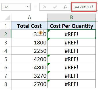
This is called the reference error and you will see this when the reference in the formula is no longer valid. This could be the case when the formula refers to a cell reference and that cell reference does not exist (happens when you delete a row/column or worksheet that was referred to in the formula).
In the below example, while the original formula was =A2/B2, when I deleted Column B, all the references to it became #REF! and it also gave the #REF! error as the result of the formula.
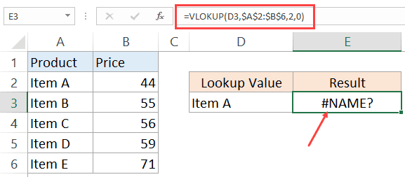
#NAME ERROR
This error is likely to a result of a misspelled function.
For example, if instead of VLOOKUP, you by mistake use VLOKUP, it will give a name error.
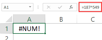
#NUM ERROR
Num error can occur if you try and calculate a very large value in Excel. For example, =187^549 will return a number error.
Another situation where you can get the NUM error is when you give a non-valid number argument to a formula. For example, if you’re calculating the Square Root if a number and you give a negative number as the argument, it will return a number error.
For example, in the case of Square Root function, if you give a negative number as the argument, it will return a number error (as shown below).
While I have shown only a couple of examples here, there can be many other reasons that can lead to errors in Excel. When you get errors in Excel, you can’t just leave it there. If the data is further used in calculations, you need to make sure the errors are handled the right way.
Excel IFERROR function is a great way to handle all types of errors in Excel.
Excel IFERROR Function – An Overview
Using the IFERROR function, you can specify what you want the formula to return instead of the error. If the formula does not return an error, then its own result is returned.
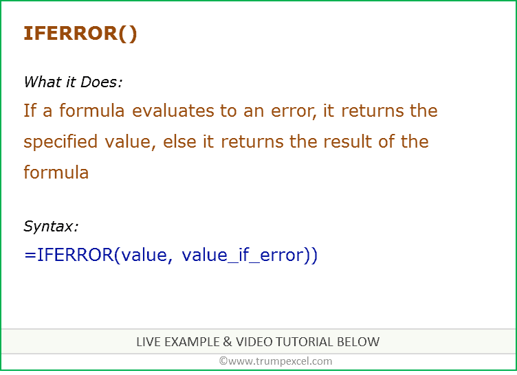
IFERROR Function Syntax
=IFERROR(value, value_if_error)
Input Arguments
- value – this is the argument that is checked for the error. In most cases, it is either a formula or a cell reference.
- value_if_error – this is the value that is returned if there is an error. The following error types evaluated: #N/A, #REF!, #DIV/0!, #VALUE!, #NUM!, #NAME?, and #NULL!.
Additional Notes:
- If you use “” as the value_if_error argument, the cell displays nothing in case of an error.
- If the value or value_if_error argument refers to an empty cell, it is treated as an empty string value by the Excel IFERROR function.
- If the value argument is an array formula, IFERROR will return an array of results for each item in the range specified in value.
Excel IFERROR Function – Examples
Here are three examples of using IFERROR function in Excel.
Example 1 – Return Blank Cell Instead of Error
If you have functions that may return an error, you can wrap it within the IFERROR function and specify blank as the value to return in case of an error.
In the example shown below, the result in D4 is the #DIV/0! error as the divisor is 0.
In this case, you can use the following formula to return blank instead of the ugly DIV error.
=IFERROR(A1/A2,””)
This IFERROR function would check whether the calculation leads to an error. If it does, it simply returns a blank as specified in the formula.
Here, you can also specify any other string or formula to display instead of the blank.
For example, the below formula would return the text “Error”, instead of the blank cell.
=IFERROR(A1/A2,”Error”)

Note: If you are using Excel 2003 or a prior version, you will not find the IFERROR function in it. In such cases, you need to use the combination of IF function and ISERROR function.
Example 2 – Return ‘Not Found’ when VLOOKUP Can’t Find a Value
When you use the Excel VLOOKUP Function, and it can’t find the lookup value in the specified range, it would return the #N/A error.
For example, below is a data set of student names and their marks. I have used the VLOOKUP function to fetch the marks of three students (in D2, D3, and D4).
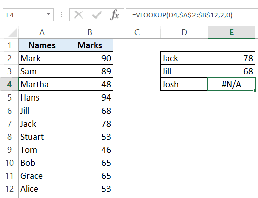
While the VLOOKUP formula in the above example finds the names of first two students, it can’t find Josh’s name on the list and hence it returns the #N/A error.
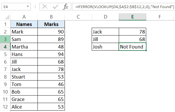
Here, we can use the IFERROR function to return a blank or some meaningful text instead of the error.
Below is the formula that will return ‘Not Found’ instead of the error.
=IFERROR(VLOOKUP(D2,$A$2:$B$12,2,0),”Not Found”)
Note that you can also use IFNA instead of IFERROR with VLOOKUP. While IFERROR would treat all kinds of error values, IFNA would only work on the #N/A errors and wouldn’t work with other errors.
Example 3 – Return 0 in case of an Error
If you don’t specify the value to return by IFERROR in the case of an error, it would automatically return 0.
For example, if I divide 100 with 0 as shown below, it would return an error.
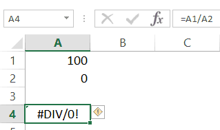
However, if I use the below IFERROR function, it would return a 0 instead. Note that you still need to use a comma after the first argument.
Example 4 – Using Nested IFERROR with VLOOKUP
Sometimes when using VLOOKUP, you may have to look through the fragmented table of arrays. For example, suppose you have the sales transaction records in 2 separate worksheets and you want to look-up an item number and see it’s value.
Doing this requires using nested IFERROR with VLOOKUP.
Suppose you have a dataset as shown below:
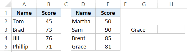
In this case, to find the score for Grace, you need to use the below nested IFERROR formula:
=IFERROR(VLOOKUP(G3,$A$2:$B$5,2,0),IFERROR(VLOOKUP(G3,$D$2:$E$5,2,0),"Not Found"))
This kind of formula nesting ensure that you get the value from either of the table and any error returned is handled.
Note that in case the tables are on the same worksheet, however, in a real-life example, it likely to be on different worksheets.
Excel IFERROR Function – VIDEO
Related Excel Functions:
- Excel AND Function.
- Excel OR Function.
- Excel NOT Function.
- Excel IF Function.
- Excel IFS Function.
- Excel FALSE Function.
- Excel TRUE Function.
You May Also Like the Following Excel Tutorials:
- Use IFERROR with VLOOKUP to Get Rid of #N/A Errors.
- Identify Errors Using Excel Formula Debugging.
![]()
IFERROR Function in Excel

IFERROR is an Excel Logical Function to Check if a value is an Error. IFERROR used in Excel to handle if the formula is evaluated to an Error. We can handle the Error Cells and Formulas with errors like #VALUE!,#N/A, #REF!, #DIV/0!, #NUM! #NAME? and #NULL!.
In this topic:
- Function
- Syntax
- Parameters
- Usage
- Examples
- IfError Return Values
IFERROR Function
Excel IFError Function helps to return a value if an formula returns an Error. For example, if we enter some formula in Cell, and we assume that there is some chance of getting an Error. In this case we can use IFERROR function to return something else when the formula evaluates an error.
=IFERROR(Actual Formula, Value if the formula returns an Error)
Example:
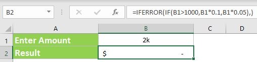
Let us say you are accepting Total Sales at Range A1 and Units in Range B1. And You wants to calculate the Unit Price at C1. Your formula at C1=A1/B1.
- If the user enters 2000 at Range A1 and 10 at B1, the formula C1 evaluates and returns the unit price as 200.
- What if the user enters 2k at Range A1 and 10 at B1, the formula C1 evaluates to an Error (#VALUE!).
- In this case, we can use IFERROR function to instruct the user to enter valid numbers.
- You can use the formula =IFERROR(A1/B1,”Please Enter Valid Number”) to ask the user to enter valid data.
Syntax
Here is the syntax of the Excel IFERROR Function. It has two required parameters.
IFERROR(value, value_if_error)
Parameters
Excel IFERROR Function takes two parameters. Value is a formula to check for an error. And the second one is the value to be returned if the first argument evaluate an error.
value: Value is a required parameter. This is the Argument which is to be evaluated for an Error. Often, it is a formula or expression.
value_if_error: This is a required parameter. This is the value to return if the formula evaluates to an error. IFERROR returns this value if the first argument evaluates to #N/A, #VALUE!, #REF!, #DIV/0!, #NUM!, #NAME? or #NULL!.
How to use IFERROR in Excel?
IFERROR Functions is used along with other Excel Functions to handle the returning error values. We can combine iferror function while using the reference functions like VLOOKUP, HLOOKUP, XLOOKUP, MATCH, INDEX. We also combine with other conditional aggregate functions like IF, COUNTIF, SUMIF, AVERAGEIF.
Using IFERROR in EXCEL Formula
Let us see how to use IFERROR Function in Excel. We can use the IFERROR function in Excel formula to find if an expression is returning an Error. You can use the IFERROR function to identify the expressions witch may return errors and handle it. IFERROR returns a value you specify if a formula evaluates to an error; otherwise, it returns the result of the formula.
- IFERROR returns a specified value if a formula evaluates to an error; otherwise, it returns the result of the formula
- We can provide a Value , a string or another Expression if the Formula evaluate to an Error
- Often, we use IFERROR with the formulas which may return errors in some (unknown) cases or wrong data inputs. And return some text or value when the formula returns an Error.
Using IFERROR with IF Statement
We can use IFERROR with IF Statement to make conditional and logical checks. Let us see how to use iferror with if statement in Excel formula.
The following example shows how to use IFERROR with IF Statement. User enter some amount at Range B1 and the If formula calculates the Discount Price as Result.
IF Formula =IF(B1>1000,B1*0.1,B1*0.05)
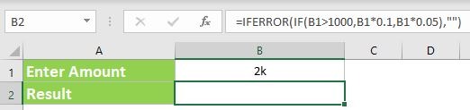
IFERROR + IF Formula =IFERROR(IF(B1>1000,B1*0.1,B1*0.05),”Please Enter Valid Data”)
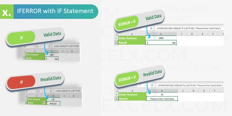
- IF Formula – Valid Data: Calculates and Result the when you enter valid data
- IF Formula – Invalid Data: Calculates and Result the error (#VALUE!) when you enter invalid number.
- IFERROR+IF Formula – Valid Data: Calculates and Result the when you enter valid data
- IFERROR+ IF Formula – Invalid Data: If you enter invalid number, IF Function calculates and Result the error (#VALUE!), IFERROR Evaluates the error and creates the custom message (“Please Enter Valid Data”).
IFERROR Blank
IFERROR Function is used to produce a Blank string if the formula evaluates an Error. Here is the IFERROR Blank Example formula which is common use of IFERROR Function.
Excel If Error Then Blank: If there is any error in the formula then Excel returns Blank using IFERROR. We will take the simple formula to return blank when there is an Error in Excel Formula. To produce a blank string, you can pass the blank string in the second argument of the IFERROR function. Or, you can simply leave the second parameter empty.
Blank String: The following formula will result a BLANK string if the the expression evaluates an Error. Here, we are providing an Blank string character(“”) as the second parameter of the IFERROR Function.
Empty Argument:The following formula will result an Empty Cell if the the expression evaluates an Error. Here, we are not providing the second parameter of the IFERROR Function. We are just closing the function after the comma.
Difference between Providing the Second Argument and Leaving Empty: Function creates a Blank String Character(“”), overwrites the default cell format when you pass the second character. If you leave empty, this will creates cell with default format (as if you entered nothing in the cell).
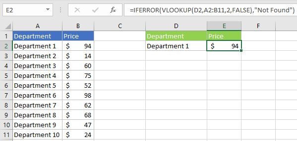
IFERROR VLOOKUP
IFERROR is used with the combination of VLOOKUP function. VLOOKUP function returns an error value (#NA) if it is not found the lookup value in the lookup table array range. We can suppress these errors using IFERROR function with VLOOKUP. Otherwise, we can perform another operation if Vlookup returns an Error.
Let us see an example to understand how to use IFERROR and VLOOKUP together. VLOOKUP tries to find the lookup value (D2) in the lookup table array (A2:B11) and returns the corresponding value in column 2. If VLOOKUP not find the value in the given range, IFERROR Returns a string (“Not found”)
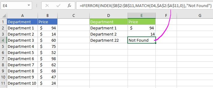
IFERROR INDEX MATCH
We use INDEX and MATCH Functions to create Advanced VLOOKUP Formula. We can use IFERROR with the combination of INDEX and MATCH functions (as used in the VLOOKUP function). INDEX and MATH Lookup functions returns an error value (#NA) if the lookup value is not found the lookup range. We can use IFERROR function to produce the alternative string.
Here is a simple example to show you how to use IFERROR function along with INDEX and MATCH reference functions. MATCH function returns the match position of the lookup value (D4) in the lookup range ($A$2:$A$11). And the INDEX function returns the value from the reference ($B$2:$B$11) from the row number returned by MATCH function. Match returns #NA error if the given lookup value is not found in the lookup range. We can use IFERROR to Returns a new string (“Not found”)
IF And IFERROR Combined
We can Combine IF and IFERROR Functions in Excel to create issue free Formulas. We can check some expression using IF Function. And trap the result using IFERROR function.
This formula will checks an expression using IF and returns the defined value. If it returns an error, error message will be displayed in the Cell.
IF IFERROR and VLOOKUP
We can also Combine IF, IFERROR Functions with VLOOKUP in Excel to create advanced Formulas. VLOOKUP fetch a value from table range. And the IFERROR Evaluates the VLOOKUP output. Finally, IF functions makes the decision to display the value based on the result.
Here is real-time example to understand how to use IFERROR and VLOOKUP together in the same formula.
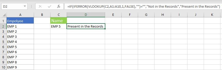
- In this formula, VLOOKUP will check for an EMP Record
- IFERROR returns blank if no record is found
- IF statement will display the message based on the result
Nested IFERROR
Nested IFERROR formula is helpful to fetch the values from multiple references. Following is the example of Nested IFERROR with VLOOKUP function to check for a value in two different ranges and return the corresponding column value. If the lookup values is not found in both the ranges, return custom value or a text.
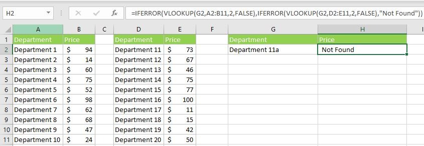
- VLOOKUP(G2,A2:B11,2,FALSE) : checks for a value G2 in the first range A2:B11
- =IFERROR(VLOOKUP(G2,A2:B11,2,FALSE), : This will checks the return value and out put the corresponding value. If it is not found in the given range (A2:B11). IFERROR process the second part of the formula (i.e; IFERROR(VLOOKUP(G2,D2:E11,2,FALSE),”Not Found”))
- VLOOKUP(G2,D2:E11,2,FALSE):checks for a value G2 in the first range D2:E11
- IFERROR(VLOOKUP(G2,D2:E11,2,FALSE),”Not Found”) : This will checks the return value of 2nd VLOOKUP and out put the corresponding value. If it is not found in the given range (D2:E11). IFERROR process the second argument of the function and returns the string “Not Found”
Nested IFERROR and IF
We can add the IF Function with Nested IFERROR function to return the value based on the result. We can use the above formula and display the value in the cell using IF Function.
Here, we have added Function to display a message as “Need to Add”,”Exist in the Table” based on the Nested IfError and If function.
Excel IFERROR Else
We can make use of this formula to check if an expression evaluates an Error then display some value. Else display another Value.
Comparing IFERROR with Other Function
We have many functions to handle the Errors in Excel. Let us see the different Error trapping Functions in Excel and how they are different from IFERROR function.
ISERROR vs IFERROR
ISERROR Function is useful to check if an expression evaluates to an error or not. IFERROR Helps to replace that error with some value.
IF ISERROR vs IFERROR
If ISERROR combination is useful when you wants to check an expression and execute Expression One when it is True and Expression Two when it is False.
IFNA vs IFERROR
IFNA Function is used when you wants to replace only if an expression returns #NA Error. Where as IFERROR is helps to tackle with any type of errors listed above.
ISNA vs IFERROR
ISNA Function is used to check if an expression is Returning a #NA type Error. IFERROR is used to replace an error if the expression evaluates to any error listed above.
IF and IFERROR
IF Function is used to check a condition and executes the first expression when it is True and the second expression when it is False. But IFERROR is used when you want to replace an error only if the expression evaluates to any error listed above.
IFERROR vs IFNA for VLOOKUP
VlookUp returns #NA type error if the lookup value is not found in the table array. You can use IFNA function to deal with this situation. But, in some cases the VlookUp return other type of Errors like #Name (based on the input expressions). You can use IfError to deal with any type of Errors as mention above.
How Does IFERROR Work
IFERROR Works as error handling formula in Excel. Following is the process flow chart of IFERROR Function with clear instructions.
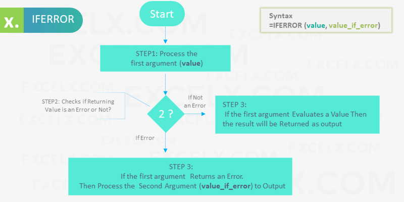
- It required two arguments to process the function
- It will process the first argument and validate the evaluated value
- If the first argument returns the value which is not an error (#VALUE!,#N/A, #REF!, #DIV/0!, #NUM! #NAME? and #NULL!.), then it returns the result output of the first argument
- If the first argument returns an error, then it will process the second argument of the IFERROR function and returns the output
Here are the simple examples to understand how does IFERROR function Works. The first example returns the actual value, and the second example returns the IFERROR function value.
Example 1: We have provided the First argument as 25+75, tried to add number and number. It returns the values as 100. So, the IFERROR function Returns the first argument.
Formula
Output:100
Example 2: We have provided the First argument as 25+”Some Text”, tried to add number and string. It returns an Error. So, the IFERROR function Returns the second argument.
Formula
Output:”You can not add a number and Text”
IFERROR Examples
1. Display Message to User
Here is a simple example to explain the IFERROR Function. The following Formula check the first expression and returns the given string as it evaluates an Error.
Formula:
=IFERROR(5/0,”Please Enter Valid Number”)Returns: Please Enter Valid Number
We can see the first argument of the formula (5/0) evaluates #DIV/0! Error. And IFERROR function trap this error and returns the second argument.
2. IFERROR Then Return 0
Let us say we are performing a calculation based on the result. If there is any Error in the Formula, we want the Excel to return Zero. In this case we can use iferror and simply return 0 if the formula evaluates to an Error.
Formula:
Returns: 0 (if the formula evaluates to an error)
3. IFERROR, Make the Cell Blank
Excel sheet do not look good if there are many Error Cells . We can use the IFERROR formula to return a blank if the formula returns errors.
Formula:
Returns: “” (if the formula evaluates to an error)
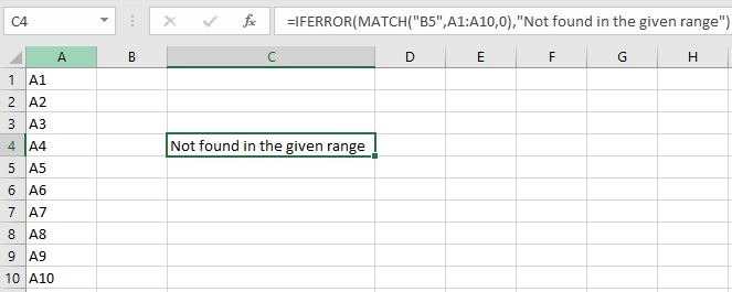
4. Check if a value found in List of values
IFEEROR helps to determine if an item found in the list of items, range or Array. The following Example checks if value find in a range of values.
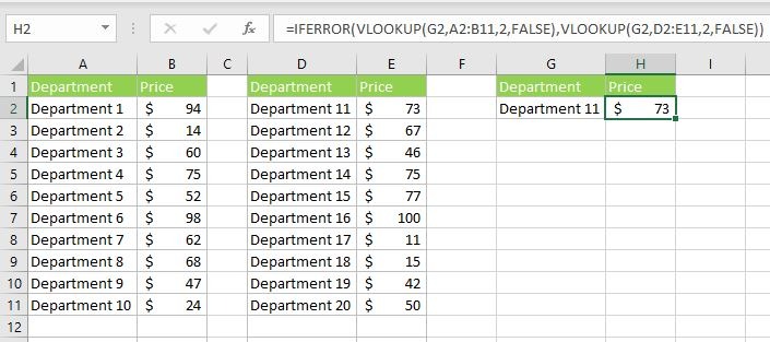
5. If Error then Evaluate another Formula
The following formula checks for a value in Range A1:A10. If it is not found in the A1:B10, IFERROR helps to check in another Range(D1:E10). Here is a simple example on IFERROR to return a value from one of the Ranges.
IFERROR Return Values
Excel IFERROR can be used to return values based on our requirement. We can return a string, a number, or evaluate a formula. Let us see the most widely returning Values of IFERROR Function.
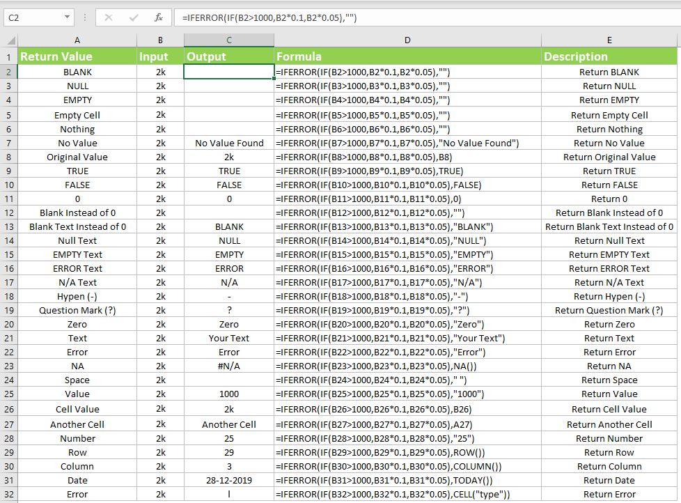
| Return Value | Formula | Description |
|---|---|---|
| BLANK | =IFERROR(IF(B2>1000,B2*0.1,B2*0.05),””) | Return BLANK
IfError Then BLANK |
| NULL | =IFERROR(IF(B3>1000,B3*0.1,B3*0.05),””) | Return NULL
IfError Then NULL |
| EMPTY | =IFERROR(IF(B4>1000,B4*0.1,B4*0.05),””) | Return EMPTY
IfError Then EMPTY |
| Empty Cell | =IFERROR(IF(B5>1000,B5*0.1,B5*0.05),””) | Return Empty Cell
IfError Then Empty Cell |
| Nothing | =IFERROR(IF(B6>1000,B6*0.1,B6*0.05),””) | Return Nothing
IfError Then Nothing |
| No Value | =IFERROR(IF(B7>1000,B7*0.1,B7*0.05),”No Value Found”) | Return No Value
IfError Then No Value |
| Original Value | =IFERROR(IF(B8>1000,B8*0.1,B8*0.05),B8) | Return Original Value
IfError Then Original Value |
| TRUE | =IFERROR(IF(B9>1000,B9*0.1,B9*0.05),TRUE) | Return TRUE
IfError Then TRUE |
| FALSE | =IFERROR(IF(B10>1000,B10*0.1,B10*0.05),FALSE) | Return FALSE
IfError Then FALSE |
| 0 | =IFERROR(IF(B11>1000,B11*0.1,B11*0.05),0) | Return 0
IfError Then 0 |
| Blank Instead of 0 | =IFERROR(IF(B12>1000,B12*0.1,B12*0.05),””) | Return Blank Instead of 0
IfError Then Blank Instead of 0 |
| Blank Text Instead of 0 | =IFERROR(IF(B13>1000,B13*0.1,B13*0.05),”BLANK”) | Return Blank Text Instead of 0
IfError Then Blank Text Instead of 0 |
| Null Text | =IFERROR(IF(B14>1000,B14*0.1,B14*0.05),”NULL”) | Return Null Text
IfError Then Null Text |
| EMPTY Text | =IFERROR(IF(B15>1000,B15*0.1,B15*0.05),”EMPTY”) | Return EMPTY Text
IfError Then EMPTY Text |
| ERROR Text | =IFERROR(IF(B16>1000,B16*0.1,B16*0.05),”ERROR”) | Return ERROR Text
IfError Then ERROR Text |
| N/A Text | =IFERROR(IF(B17>1000,B17*0.1,B17*0.05),”N/A”) | Return N/A Text
IfError Then N/A Text |
| Hyphen (-) | =IFERROR(IF(B18>1000,B18*0.1,B18*0.05),”-“) | Return Hyphen (-)
IfError Then Hyphen (-) |
| Question Mark (?) | =IFERROR(IF(B19>1000,B19*0.1,B19*0.05),”?”) | Return Question Mark (?)
IfError Then Question Mark (?) |
| Zero | =IFERROR(IF(B20>1000,B20*0.1,B20*0.05),”Zero”) | Return Zero
IfError Then Zero |
| Text | =IFERROR(IF(B21>1000,B21*0.1,B21*0.05),”Your Text”) | Return Text
IfError Then Text |
| Error | =IFERROR(IF(B22>1000,B22*0.1,B22*0.05),”Error”) | Return Error
IfError Then Error |
| NA | =IFERROR(IF(B23>1000,B23*0.1,B23*0.05),NA()) | Return NA
IfError Then NA |
| Space | =IFERROR(IF(B24>1000,B24*0.1,B24*0.05),” “) | Return Space
IfError Then Space |
| Value | =IFERROR(IF(B25>1000,B25*0.1,B25*0.05),”1000″) | Return Value
IfError Then Value |
| Cell Value | =IFERROR(IF(B26>1000,B26*0.1,B26*0.05),B26) | Return Cell Value
IfError Then Cell Value |
| Another Cell | =IFERROR(IF(B27>1000,B27*0.1,B27*0.05),A27) | Return Another Cell
IfError Then Another Cell |
| Number | =IFERROR(IF(B28>1000,B28*0.1,B28*0.05),”25″) | Return Number
IfError Then Number |
| Row | =IFERROR(IF(B29>1000,B29*0.1,B29*0.05),ROW()) | Return Row
IfError Then Row |
| Column | =IFERROR(IF(B30>1000,B30*0.1,B30*0.05),COLUMN()) | Return Column
IfError Then Column |
| Date | =IFERROR(IF(B31>1000,B31*0.1,B31*0.05),TODAY()) | Return Date
IfError Then Date |
| Error | =IFERROR(IF(B32>1000,B32*0.1,B32*0.05),CELL(“type”)) | Return Error
IfError Then Error |
Return 0:
We can use IFERROR to return 0 if the formula evaluates an Error. This is very helpful while processing the numerical data. If you have the formulas witch are resulting an Error while calculation, it will effect the all other calculations. If you return 0 using IFERROR, you can avoid those issues with your spreadsheet.
Formula:
Return Blank:
If you are dealing with string data, you can return blank instead of 0. It makes your sheet more cleaner and issue free. Following is the formula to Return Blank if there are any errors in Formula.
Formula:
Return Null:
You can make use of IFERROR and return Null string to avoid conflicts with other formula. Here is
Best Practices
Please remember the following best practices to be followed while using IFERROR in Excel Formula.
- IFERROR is very important and useful formula to create an issue free spreadsheet worksheet. Use this formula when there is a chance of evaluation error.
- Try to use smaller portion of the formula, instead of the entire formula.
- Do not leave the arguments empty. IFERROR treats the empty arguments as an Empty String (“”).
- Try to Avoid using IF + ISERROR , instead use IFERROR Function
- Use ISNA function to check if the expression evaluates only #NA Error, otherwise use IFERROR to catch all Errors
- ISERR function to check if the expression evaluates errors except #NA Error
Share This Story, Choose Your Platform!
© Copyright 2012 – 2020 | Excelx.com | All Rights Reserved
Page load link