
The IF function allows you to make a logical comparison between a value and what you expect by testing for a condition and returning a result if that condition is True or False.
-
=IF(Something is True, then do something, otherwise do something else)
But what if you need to test multiple conditions, where let’s say all conditions need to be True or False (AND), or only one condition needs to be True or False (OR), or if you want to check if a condition does NOT meet your criteria? All 3 functions can be used on their own, but it’s much more common to see them paired with IF functions.
Use the IF function along with AND, OR and NOT to perform multiple evaluations if conditions are True or False.
Syntax
-
IF(AND()) — IF(AND(logical1, [logical2], …), value_if_true, [value_if_false]))
-
IF(OR()) — IF(OR(logical1, [logical2], …), value_if_true, [value_if_false]))
-
IF(NOT()) — IF(NOT(logical1), value_if_true, [value_if_false]))
|
Argument name |
Description |
|
|
logical_test (required) |
The condition you want to test. |
|
|
value_if_true (required) |
The value that you want returned if the result of logical_test is TRUE. |
|
|
value_if_false (optional) |
The value that you want returned if the result of logical_test is FALSE. |
|
Here are overviews of how to structure AND, OR and NOT functions individually. When you combine each one of them with an IF statement, they read like this:
-
AND – =IF(AND(Something is True, Something else is True), Value if True, Value if False)
-
OR – =IF(OR(Something is True, Something else is True), Value if True, Value if False)
-
NOT – =IF(NOT(Something is True), Value if True, Value if False)
Examples
Following are examples of some common nested IF(AND()), IF(OR()) and IF(NOT()) statements. The AND and OR functions can support up to 255 individual conditions, but it’s not good practice to use more than a few because complex, nested formulas can get very difficult to build, test and maintain. The NOT function only takes one condition.

Here are the formulas spelled out according to their logic:
|
Formula |
Description |
|---|---|
|
=IF(AND(A2>0,B2<100),TRUE, FALSE) |
IF A2 (25) is greater than 0, AND B2 (75) is less than 100, then return TRUE, otherwise return FALSE. In this case both conditions are true, so TRUE is returned. |
|
=IF(AND(A3=»Red»,B3=»Green»),TRUE,FALSE) |
If A3 (“Blue”) = “Red”, AND B3 (“Green”) equals “Green” then return TRUE, otherwise return FALSE. In this case only the first condition is true, so FALSE is returned. |
|
=IF(OR(A4>0,B4<50),TRUE, FALSE) |
IF A4 (25) is greater than 0, OR B4 (75) is less than 50, then return TRUE, otherwise return FALSE. In this case, only the first condition is TRUE, but since OR only requires one argument to be true the formula returns TRUE. |
|
=IF(OR(A5=»Red»,B5=»Green»),TRUE,FALSE) |
IF A5 (“Blue”) equals “Red”, OR B5 (“Green”) equals “Green” then return TRUE, otherwise return FALSE. In this case, the second argument is True, so the formula returns TRUE. |
|
=IF(NOT(A6>50),TRUE,FALSE) |
IF A6 (25) is NOT greater than 50, then return TRUE, otherwise return FALSE. In this case 25 is not greater than 50, so the formula returns TRUE. |
|
=IF(NOT(A7=»Red»),TRUE,FALSE) |
IF A7 (“Blue”) is NOT equal to “Red”, then return TRUE, otherwise return FALSE. |
Note that all of the examples have a closing parenthesis after their respective conditions are entered. The remaining True/False arguments are then left as part of the outer IF statement. You can also substitute Text or Numeric values for the TRUE/FALSE values to be returned in the examples.
Here are some examples of using AND, OR and NOT to evaluate dates.

Here are the formulas spelled out according to their logic:
|
Formula |
Description |
|---|---|
|
=IF(A2>B2,TRUE,FALSE) |
IF A2 is greater than B2, return TRUE, otherwise return FALSE. 03/12/14 is greater than 01/01/14, so the formula returns TRUE. |
|
=IF(AND(A3>B2,A3<C2),TRUE,FALSE) |
IF A3 is greater than B2 AND A3 is less than C2, return TRUE, otherwise return FALSE. In this case both arguments are true, so the formula returns TRUE. |
|
=IF(OR(A4>B2,A4<B2+60),TRUE,FALSE) |
IF A4 is greater than B2 OR A4 is less than B2 + 60, return TRUE, otherwise return FALSE. In this case the first argument is true, but the second is false. Since OR only needs one of the arguments to be true, the formula returns TRUE. If you use the Evaluate Formula Wizard from the Formula tab you’ll see how Excel evaluates the formula. |
|
=IF(NOT(A5>B2),TRUE,FALSE) |
IF A5 is not greater than B2, then return TRUE, otherwise return FALSE. In this case, A5 is greater than B2, so the formula returns FALSE. |

Using AND, OR and NOT with Conditional Formatting
You can also use AND, OR and NOT to set Conditional Formatting criteria with the formula option. When you do this you can omit the IF function and use AND, OR and NOT on their own.
From the Home tab, click Conditional Formatting > New Rule. Next, select the “Use a formula to determine which cells to format” option, enter your formula and apply the format of your choice.

Using the earlier Dates example, here is what the formulas would be.

|
Formula |
Description |
|---|---|
|
=A2>B2 |
If A2 is greater than B2, format the cell, otherwise do nothing. |
|
=AND(A3>B2,A3<C2) |
If A3 is greater than B2 AND A3 is less than C2, format the cell, otherwise do nothing. |
|
=OR(A4>B2,A4<B2+60) |
If A4 is greater than B2 OR A4 is less than B2 plus 60 (days), then format the cell, otherwise do nothing. |
|
=NOT(A5>B2) |
If A5 is NOT greater than B2, format the cell, otherwise do nothing. In this case A5 is greater than B2, so the result will return FALSE. If you were to change the formula to =NOT(B2>A5) it would return TRUE and the cell would be formatted. |
Note: A common error is to enter your formula into Conditional Formatting without the equals sign (=). If you do this you’ll see that the Conditional Formatting dialog will add the equals sign and quotes to the formula — =»OR(A4>B2,A4<B2+60)», so you’ll need to remove the quotes before the formula will respond properly.
Need more help?

See also
You can always ask an expert in the Excel Tech Community or get support in the Answers community.
Learn how to use nested functions in a formula
IF function
AND function
OR function
NOT function
Overview of formulas in Excel
How to avoid broken formulas
Detect errors in formulas
Keyboard shortcuts in Excel
Logical functions (reference)
Excel functions (alphabetical)
Excel functions (by category)
Things will not always be the way we want them to be. The unexpected can happen. For example, let’s say you have to divide numbers. Trying to divide any number by zero (0) gives an error. Logical functions come in handy such cases. In this tutorial, we are going to cover the following topics.
In this tutorial, we are going to cover the following topics.
- What is a Logical Function?
- IF function example
- Excel Logic functions explained
- Nested IF functions
What is a Logical Function?
It is a feature that allows us to introduce decision-making when executing formulas and functions. Functions are used to;
- Check if a condition is true or false
- Combine multiple conditions together
What is a condition and why does it matter?
A condition is an expression that either evaluates to true or false. The expression could be a function that determines if the value entered in a cell is of numeric or text data type, if a value is greater than, equal to or less than a specified value, etc.
IF Function example
We will work with the home supplies budget from this tutorial. We will use the IF function to determine if an item is expensive or not. We will assume that items with a value greater than 6,000 are expensive. Those that are less than 6,000 are less expensive. The following image shows us the dataset that we will work with.
 and conditions in Excel")
- Put the cursor focus in cell F4
- Enter the following formula that uses the IF function
=IF(E4<6000,”Yes”,”No”)
HERE,
- “=IF(…)” calls the IF functions
- “E4<6000” is the condition that the IF function evaluates. It checks the value of cell address E4 (subtotal) is less than 6,000
- “Yes” this is the value that the function will display if the value of E4 is less than 6,000
-
“No” this is the value that the function will display if the value of E4 is greater than 6,000
When you are done press the enter key
You will get the following results
 and conditions in Excel")
Excel Logic functions explained
The following table shows all of the logical functions in Excel
| S/N | FUNCTION | CATEGORY | DESCRIPTION | USAGE |
|---|---|---|---|---|
| 01 | AND | Logical | Checks multiple conditions and returns true if they all the conditions evaluate to true. | =AND(1 > 0,ISNUMBER(1)) The above function returns TRUE because both Condition is True. |
| 02 | FALSE | Logical | Returns the logical value FALSE. It is used to compare the results of a condition or function that either returns true or false | FALSE() |
| 03 | IF | Logical |
Verifies whether a condition is met or not. If the condition is met, it returns true. If the condition is not met, it returns false. =IF(logical_test,[value_if_true],[value_if_false]) |
=IF(ISNUMBER(22),”Yes”, “No”) 22 is Number so that it return Yes. |
| 04 | IFERROR | Logical | Returns the expression value if no error occurs. If an error occurs, it returns the error value | =IFERROR(5/0,”Divide by zero error”) |
| 05 | IFNA | Logical | Returns value if #N/A error does not occur. If #N/A error occurs, it returns NA value. #N/A error means a value if not available to a formula or function. |
=IFNA(D6*E6,0) N.B the above formula returns zero if both or either D6 or E6 is/are empty |
| 06 | NOT | Logical | Returns true if the condition is false and returns false if condition is true |
=NOT(ISTEXT(0)) N.B. the above function returns true. This is because ISTEXT(0) returns false and NOT function converts false to TRUE |
| 07 | OR | Logical | Used when evaluating multiple conditions. Returns true if any or all of the conditions are true. Returns false if all of the conditions are false |
=OR(D8=”admin”,E8=”cashier”) N.B. the above function returns true if either or both D8 and E8 admin or cashier |
| 08 | TRUE | Logical | Returns the logical value TRUE. It is used to compare the results of a condition or function that either returns true or false | TRUE() |
A nested IF function is an IF function within another IF function. Nested if statements come in handy when we have to work with more than two conditions. Let’s say we want to develop a simple program that checks the day of the week. If the day is Saturday we want to display “party well”, if it’s Sunday we want to display “time to rest”, and if it’s any day from Monday to Friday we want to display, remember to complete your to do list.
A nested if function can help us to implement the above example. The following flowchart shows how the nested IF function will be implemented.
 and conditions in Excel")
The formula for the above flowchart is as follows
=IF(B1=”Sunday”,”time to rest”,IF(B1=”Saturday”,”party well”,”to do list”))
HERE,
- “=IF(….)” is the main if function
- “=IF(…,IF(….))” the second IF function is the nested one. It provides further evaluation if the main IF function returned false.
Practical example
 and conditions in Excel")
Create a new workbook and enter the data as shown below
 and conditions in Excel")
- Enter the following formula
=IF(B1=”Sunday”,”time to rest”,IF(B1=”Saturday”,”party well”,”to do list”))
- Enter Saturday in cell address B1
- You will get the following results
 and conditions in Excel")
Download the Excel file used in Tutorial
Summary
Logical functions are used to introduce decision-making when evaluating formulas and functions in Excel.
This article will explain how to use the conditional functions IF, AND, OR and NOT on Microsoft Excel. Each of these functions can be used as part of a formula in a cell to compare data samples in any number of columns or sheets in an Excel file. For ease of understanding, we have also included a visual map that illustrates how simple changes in each formula affects your results.
IF function
The IF function allows you to apply a condition to your data whereby one result is returned if your condition is TRUE and another result if the condition is FALSE. IF functions can be either isolated, meaning that only one condition is applied to your data, or nested, where multiple criteria are applied to generate a TRUE or FALSE result.
Isolated IF function
Here are two examples of an isolated IF function. In these examples, we are only applying one condition to generate our results:
If the grade in column A1 is greater than or equal to 19, then display 20; otherwise, display A1. = IF (A1> = 19, 20, A1)
If the data in A1 is «Discount», then subtract 10%, otherwise keep A1. = A1 * IF (A1 = «Discount»; 1-10%; 1)
Nested IF function
Here are some examples of a nested IF function. In these cases, multiple IF functions are applied to the data, generating one of several responses depending on the data housed in the data constant. You’ll notice that each criteria is separated by the use of a semicolon, and that the number of parentheses used at the end of our formula is dependent on the number of functions «nested» inside:
If the grade in A1 is greater than 12, then display «continue»; if A1 > 18, then display «very good», otherwise display «satisfactory». But if A1 <= 12, then display «improve».
=IF(A1>12;»continue,» & IF(A1>18;»very good»;»satisfactory»);»improve»)
or
=IF(A1<12;»continue»;IF (A1<18;»continue, satisfactory»;»continue, very good»))
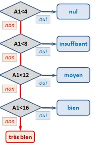
If the grade in A1 is less than 4, then display «poor» ; if A1 is between 4 and 8, display «Unsatisfactory» ; if A1 is between 8 and 12, display «OK» ; if A1 is between 12 and 16, display «Good» ; if not, display «Very Good».
=IF(A1<4;»Poor»;SI(A1<8;»Unsatisfactory»;IF(A1<12;»OK»;SI(A1<16;»Good»;»Very Good»))))
AND function
Unlike an IF function, which can function in isolation with one given condition, the AND function tests a plurality of user-defined conditions and returns TRUE if all data conditions are met, and FALSE if even one condition is not met.
Similar to other conditional formulas, you do have the capability to define your own results for TRUE and FALSE. Here’s an example:
Show «The Countess!» if all of these conditions are met: A2 (sex) = woman, B2 (status) = married, C2 (spouse) = count and D2 (score) = present; if not, display «Hello!»:
=IF(And(A2=»woman»;B2=»married»; C2=»count»; D2=»present»); «The Countess!»; «Hello!»)

You’ll note that this formula begins with the IF function. This use of IF signals to Excel that we are about to apply some sort of logical formula. Immediately following the IF function is our AND function and our data, grouped in the same set of parentheses to isolate the functions. Note that the «TRUE» condition («The Countess!») is listed before the «FALSE» condition (Hello!). Both results are separated by a semicolon and are included in the parentheses.
OR function
The OR function tests user-defined conditions and returns TRUE (or similar) if any of the conditions stipulated by the user are met, and FALSE (or similar) if none of the conditions apply. The OR function is much less absolute than the AND function. Here’s an example:
Display «Pilot» if A3 contains one of the following conditions: plane, formula 1, motor; display «Conductor» if A3 contains car or work; if not, display «?»
=IF(OR(A3=»plane»;A3=»formula 1″; A3=»motor»);»Pilot»; IF(OR(A3=»car»;A3=»work»);»Conductor»;»?»))
NOT function
The NOT function returns an opposite value of a user supplied logical value or expression.
The formula =IF(ENT(A3)=A3; «whole»;»decimal») could also be written as =IF(NOT(ENT(A3)=A3); «decimal»;»whole»).
In the same way, the formula =IF(A4<>»French»;»Foreign»;»European») is equivalent to <bold>= IF(NOT(A4=»French»);»Foreign»;»European»).
Combinations
The functions AND, OR, and NOT are most often associated with the IF function.
What’s interesting (and satisfying) about these functions is that, together, they can be used to create a flow chart to serve as a visual representation of a problem’s algorithm. When using these functions, ensure that all parentheses and semicolons are correctly placed to ensure the best results.
visit our forum for more excel related themes
Logical functions are useful for calculations that require multiple conditions or criteria to test. In our earlier articles, we have seen “VBA IF,” “VBA OR,” and “VBA AND” conditions. This article will discuss the “VBA IF NOT” function. Before introducing VBA IF NOT function, let me show you about VBA NOT functionThe VBA NOT function in MS Office Excel VBA is a built-in logical function. If a condition is FALSE, it yields TRUE; otherwise, it returns FALSE. It works as an inverse function.read more first.
Table of contents
- IF NOT in VBA
- What is NOT Function in VBA?
- Examples of NOT & IF Function in VBA?
- Example #1
- Example #2
- NOT with IF Condition:
- Recommended Articles
What is NOT Function in VBA?
The “NOT” function is one of our logical functions with Excel and VBA. All the logical functions require logical tests to perform and return TRUE if the logical test is correct. If the logical test is incorrect, it will return FALSE.
But “VBA NOT” is the opposite of the other logical function. So, we would say this is the inverse function of logical functions.
The “VBA NOT” function returns “FALSE” if the logical test is correct. If the logical test is incorrect, it will return “TRUE.” Now, look at the syntax of the “VBA NOT” function.
NOT(Logical Test)
It is very simple. First, we need to provide a logical test. Then, the NOT function evaluates the test and returns the result.
Examples of NOT & IF Function in VBA?
Below are the examples of using the IF and NOT function in excelNOT Excel function is a logical function in Excel that is also known as a negation function and it negates the value returned by a function or the value returned by another logical function.read more VBA.
You can download this VBA IF NOT Excel Template here – VBA IF NOT Excel Template
Example #1
Take a look at the below code for an example.
Code:
Sub NOT_Example()

  Dim k As String

  k = Not (100 = 100)

  MsgBox k

End Sub
In the above code, we have declared the variable as a string.
Dim k As String
Then, for this variable, we have assigned the NOT function with the logical test as 100 = 100.
k = Not (100 = 100)
Then, we have written the code to show the result in the VBA message boxVBA MsgBox function is an output function which displays the generalized message provided by the developer. This statement has no arguments and the personalized messages in this function are written under the double quotes while for the values the variable reference is provided.read more. MsgBox k
Now, we will execute the code and see the result.

We got the result as “FALSE.”
Now, look back at the logical testA logical test in Excel results in an analytical output, either true or false. The equals to operator, “=,” is the most commonly used logical test.read more. We have provided the logical test as 100 = 100, which is generally TRUE; since we had given the NOT function, we got the result as FALSE. As we said in the beginning, it gives inverse results compared to other logical functions. Since 100 equals 100, it has returned the result as FALSE.
Example #2
Now, we will look at one more example with different numbers.
Code:
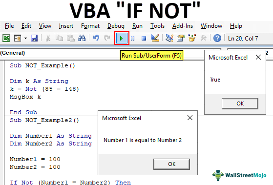
Sub NOT_Example()

 Dim k As String

 k = Not (85 = 148)

 MsgBox k

End Sub
The code is the same. The only thing we have changed here is We have changed the logical test from 100 = 100 to 85 = 148.
Now, we will run the code and see what the result is.

This time we got the result as TRUE. Now, examine the logical test.
k = Not (85 = 148)
We all know 85 is not equal to the number 148. Since it is not equal, the NOT function has returned the result as TRUE.
NOT with IF Condition:
In Excel or VBA, logical conditions are incomplete without the combination IF condition. Using the IF condition in excelIF function in Excel evaluates whether a given condition is met and returns a value depending on whether the result is “true” or “false”. It is a conditional function of Excel, which returns the result based on the fulfillment or non-fulfillment of the given criteria.
read more we can do many more things beyond default TRUE or FALSE. For example, we got FALSE and TRUE default results in the above examples. Instead, we can modify the result in our own words.
Look at the below code.
Code:
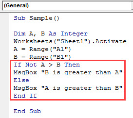
Sub NOT_Example2()

  Dim Number1 As String
  Dim Number2 As String

  Number1 = 100
  Number2 = 100

  If Not (Number1 = Number2) Then
   MsgBox "Number 1 is not equal to Number 2"
  Else
   MsgBox "Number 1 is equal to Number 2"
  End If

End Sub
We have declared two variables.
Dim Number1 As String & Dim Number2 As String
For these two variables, we have assigned the numbers 100 and 100, respectively.
Number1 = 100 & Number2 = 100
Then, we have attached the IF condition to alter the default TRUE or FALSE for the NOT function. If the result of the NOT function is TRUE, then my result will be as follows.
MsgBox “Number 1 is not equal to Number 2.”
If the NOT function result is FALSE, my result is as follows.
MsgBox “Number 1 is equal to Number 2.”
Now, we will run the code and see what happens.
We got the result as “Number 1 is equal to Number 2”, so the NOT function has returned the FALSE result to the IF condition. So, the IF condition returned this result.
Like this, we can use the IF condition to do the inverse test.
Recommended Articles
This article has been a guide to VBA IF NOT. Here, we discuss using the IF and NOT function in Excel VBA, examples, and downloadable Excel templates. Below are some useful articles related to VBA: –
- VBA Replace String
- VBA If Else Statement
- VBA AND Function
- IF OR in VBA
VBA IF Not
In any programming language, we have logical operators AND OR and NOT. Every operator has a specific function to do. AND combines two or more statements and return values true if every one of the statements is true where is in OR operator if any one of the statements is true the value is true. The NOT operator is a different thing. NOT operator negates the given statement. We use these logical operators with IF statements in our day to day data analysis. If we use IF NOT statement in VBA consider this as an inverse function.
We have discussed above that we use the logical operators with if statements. In this article, we will use NOT operator with the if statement. I said earlier that IF NOT statement in VBA is also considered as an inverse function. Why is that because if the condition is true it returns false and if the condition is false it returns true. Have a look below,
IF A>B equals to IF NOT B>A
Both the if statements above are identical how? In the first statement if A is greater than B then the next statement is executed and in the next, if not statement means if B is not greater than A which in itself means A is greater than B.
The most simple way to understand IF NOT statement should be as follows:
If True Then
If NOT false Then
Or we can say that
If False then
IF NOT True then
Both the statements in Comparison 1 and Comparison 2 are identical to each other.
Let’s use IF NOT function in few examples which will make it more clearly for us.
Note: We need to keep in mind that in order to use VBA in excel we first have to enable our developer’s tab from the files tab and then from the options section.
How to Use Excel VBA IF Not?
We will learn how to use a VBA IF Not with few examples in excel.
You can download this VBA IF NOT Excel Template here – VBA IF NOT Excel Template
Example #1 – VBA IF Not
Follow the below steps to use IF NOT in Excel VBA.
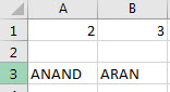
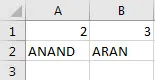
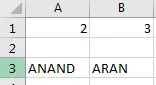
For example, I have two values in sheet 1 in cell A1 and B1. Have a look at them below,
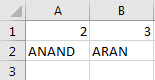
What I want to do is compare these two values which one is greater using IF NOT statement in VBA.
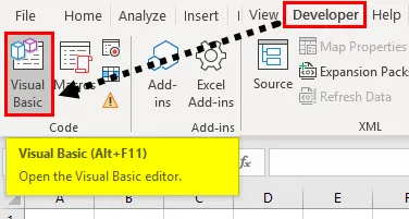
Step 1: Go to the developer’s tab and then click on Visual Basic to open the VB Editor.

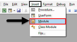
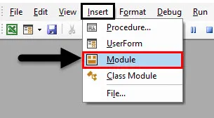
Step 2: Insert a module from the insert tab in the VB Editor. Double click on the module we just inserted to open another window where we are going to write our code.

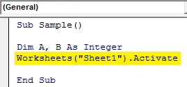
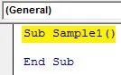
Step 3: Every VBA code starts with a sub-function as below,
Code:
Sub Sample()

End Sub
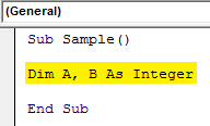
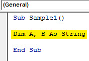
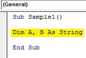
Step 4: Declare two variables as integers which will store our values from cell A1 and B1.
Code:
Sub Sample()

Dim A, B As Integer

End Sub
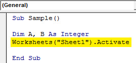
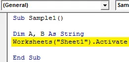
Step 5: To assign values to these variables we need to activate the worksheet first by the following code.
Code:
Sub Sample()

Dim A, B As Integer
Worksheets("Sheet1").Activate

End Sub
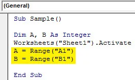
Step 6: Now we will assign these variables the values of A1 and B1.
Code:
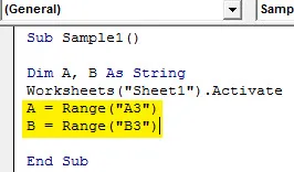
Sub Sample()

Dim A, B As Integer
Worksheets("Sheet1").Activate
A = Range("A1")
B = Range("B1")

End Sub

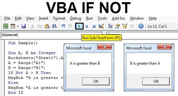
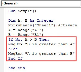
Step 7: Let us compare both the variables using IF NOT statement by the following code,
Code:
Sub Sample()

Dim A, B As Integer
Worksheets("Sheet1").Activate
A = Range("A1")
B = Range("B1")
If Not A > B Then
MsgBox "B is greater than A"
Else
MsgBox "A is greater than B"
End If

End Sub
Step 8: Run the above code from the run button in VBA or we can press the F5 button to do the same. We will get the following result.
Step 9: Let us inverse the values of A and B and again run the code to see the following result.

In the first execution, A was greater than B but we compared IF NOT A>B, Initially, the condition was true so it displayed the result for False statement i.e. A is greater than B and vice versa for execution second.
Example #2 – VBA IF Not
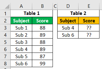
In the first example we compared integers, let us compare strings in this example with IF NOT statement in VBA. In the same sheet1, we have two strings in cell A3 and B3 as follows,
Let us compare both the strings using IF NOT Statement.
Step 1: To open VB Editor first click on Developer’s Tab and then click on Visual Basic.
Step 2: In the same module, we inserted above double click on it to start writing the second code.
Step 3: Declare a sub-function below the code we wrote first.
Code:
Sub Sample1()

End Sub

Step 4: Declare two variables as a string that will store our values from cell A3 and B3.
Code:
Sub Sample1()

Dim A, B As String

End Sub
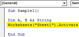
Step 5: To assign values to these variables we need to activate the worksheet first by the following code to use its properties.
Code:
Sub Sample1()

Dim A, B As String
Worksheets("Sheet1").Activate

End Sub
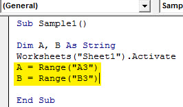
Step 6: Now we will assign these variables the values of A3 and B3.
Code:
Sub Sample1()

Dim A, B As String
Worksheets("Sheet1").Activate
A = Range("A3")
B = Range("B3")

End Sub
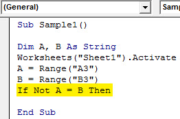
Step 7: Let us compare both the variables using IF NOT statement by the starting the if statement as follows,
Code:
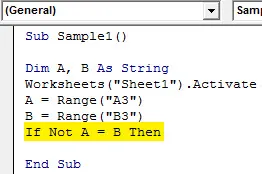
Sub Sample1()

Dim A, B As String
Worksheets("Sheet1").Activate
A = Range("A3")
B = Range("B3")
If Not A = B Then

End Sub
Step 8: If A = B condition is true then the above statement will negate it and return the value as false.
Code:
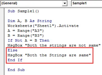
Sub Sample1()

Dim A, B As String
Worksheets("Sheet1").Activate
A = Range("A3")
B = Range("B3")
If Not A = B Then
MsgBox "Both the strings are not same"

End Sub
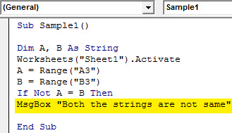
Step 9: If both the strings are same i.e. if the result is returned as true display the following message,
Code:
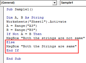
Sub Sample1()

Dim A, B As String
Worksheets("Sheet1").Activate
A = Range("A3")
B = Range("B3")
If Not A = B Then
MsgBox "Both the strings are not same"
Else
MsgBox "Both the Strings are same"
End If

End Sub
Step 10: Now let us run the above code by pressing the F5 button or from the run button given. Once we run the code we get the following result.

Step 11: Now let us make both the stings in A3 and B3 cell same to see the different result when we run the same code.
In the first execution A was not similar to B but we compared IF NOT A=B, Initially the condition was true so it displayed the result for false statement i.e. both the strings are not same and when both of the strings were same we get the different message as both the strings are same.
Things to Remember
- IF NOT is a comparison statement.
- IF NOT negates the value of the condition i.e. if a condition is true it returns false and vice versa.
- IF NOT statement is basically an inverse function.
Recommended Articles
This has been a guide to VBA If Not. Here we have discussed how to use Excel VBA If Not along with practical examples and downloadable excel template. You can also go through our other suggested articles –
- VBA Active Cell
- VBA RGB
- VBA Transpose
- VBA Not
Содержание
- Using IF with AND, OR and NOT functions
- Examples
- Using AND, OR and NOT with Conditional Formatting
- Need more help?
- See also
- Function IF in Excel with a few examples of conditions
- The syntax of the function «IF» with one condition
- The function IF in Excel with multiple conditions
- Enhanced functionality with the help of the operators «AND» and «OR»
- How to compare data in two tables
- Excel Commands
- List of Top 10 Commands in Excel
- #1 VLOOKUP Function to Fetch Data
- #2 IF Condition to Do Logical Test
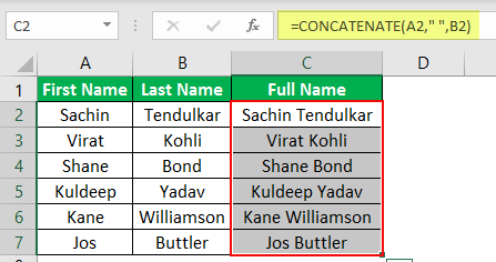
- #3 CONCATENATE Function to Combine Two or More Values
- #4 Count Only Numerical Values
- #5 Count All Values
- #6 Count Based on Condition
- #7 Count Number of Characters in the Cell
- #8 Convert Negative Value to Positive Value
- #9 Convert All Characters to UPPERCASE Values
- #10 Find Maximum and Minimum Values
- Things to Remember
- Recommended Articles
Using IF with AND, OR and NOT functions
The IF function allows you to make a logical comparison between a value and what you expect by testing for a condition and returning a result if that condition is True or False.
=IF(Something is True, then do something, otherwise do something else)
But what if you need to test multiple conditions, where let’s say all conditions need to be True or False ( AND), or only one condition needs to be True or False ( OR), or if you want to check if a condition does NOT meet your criteria? All 3 functions can be used on their own, but it’s much more common to see them paired with IF functions.
Use the IF function along with AND, OR and NOT to perform multiple evaluations if conditions are True or False.
IF(AND()) — IF(AND(logical1, [logical2], . ), value_if_true, [value_if_false]))
IF(OR()) — IF(OR(logical1, [logical2], . ), value_if_true, [value_if_false]))
IF(NOT()) — IF(NOT(logical1), value_if_true, [value_if_false]))
The condition you want to test.
The value that you want returned if the result of logical_test is TRUE.
The value that you want returned if the result of logical_test is FALSE.
Here are overviews of how to structure AND, OR and NOT functions individually. When you combine each one of them with an IF statement, they read like this:
AND – =IF(AND(Something is True, Something else is True), Value if True, Value if False)
OR – =IF(OR(Something is True, Something else is True), Value if True, Value if False)
NOT – =IF(NOT(Something is True), Value if True, Value if False)
Examples
Following are examples of some common nested IF(AND()), IF(OR()) and IF(NOT()) statements. The AND and OR functions can support up to 255 individual conditions, but it’s not good practice to use more than a few because complex, nested formulas can get very difficult to build, test and maintain. The NOT function only takes one condition.
Here are the formulas spelled out according to their logic:
=IF(AND(A2>0,B2 0,B4 50),TRUE,FALSE)
IF A6 (25) is NOT greater than 50, then return TRUE, otherwise return FALSE. In this case 25 is not greater than 50, so the formula returns TRUE.
IF A7 (“Blue”) is NOT equal to “Red”, then return TRUE, otherwise return FALSE.
Note that all of the examples have a closing parenthesis after their respective conditions are entered. The remaining True/False arguments are then left as part of the outer IF statement. You can also substitute Text or Numeric values for the TRUE/FALSE values to be returned in the examples.
Here are some examples of using AND, OR and NOT to evaluate dates.
Here are the formulas spelled out according to their logic:
IF A2 is greater than B2, return TRUE, otherwise return FALSE. 03/12/14 is greater than 01/01/14, so the formula returns TRUE.
=IF(AND(A3>B2,A3 B2,A4 B2),TRUE,FALSE)
IF A5 is not greater than B2, then return TRUE, otherwise return FALSE. In this case, A5 is greater than B2, so the formula returns FALSE.
Using AND, OR and NOT with Conditional Formatting
You can also use AND, OR and NOT to set Conditional Formatting criteria with the formula option. When you do this you can omit the IF function and use AND, OR and NOT on their own.
From the Home tab, click Conditional Formatting > New Rule. Next, select the “ Use a formula to determine which cells to format” option, enter your formula and apply the format of your choice.
Edit Rule dialog showing the Formula method» loading=»lazy»>
Using the earlier Dates example, here is what the formulas would be.
If A2 is greater than B2, format the cell, otherwise do nothing.
=AND(A3>B2,A3 B2,A4 B2)
If A5 is NOT greater than B2, format the cell, otherwise do nothing. In this case A5 is greater than B2, so the result will return FALSE. If you were to change the formula to =NOT(B2>A5) it would return TRUE and the cell would be formatted.
Note: A common error is to enter your formula into Conditional Formatting without the equals sign (=). If you do this you’ll see that the Conditional Formatting dialog will add the equals sign and quotes to the formula — =»OR(A4>B2,A4
Need more help?
See also
You can always ask an expert in the Excel Tech Community or get support in the Answers community.
Источник
Function IF in Excel with a few examples of conditions
The logical IF statement in Excel is used for the recording of certain conditions. It compares the number and / or text, function, etc. of the formula when the values correspond to the set parameters, and then there is one record, when do not respond — another.
Logic functions — it is a very simple and effective tool that is often used in practice. Let us consider it in details by examples.
The syntax of the function «IF» with one condition
The operation syntax in Excel is the structure of the functions necessary for its operation data.
Let us consider the function syntax:
- Boolean – what the operator checks (text or numeric data cell).
- Value_if_TRUE – what will appear in the cell when the text or numbers correspond to a predetermined condition (true).
- Value_if_FALSE – what appears in the box when the text or the number does not meet the predetermined condition (false).

Logical IF functions.
The operator checks the A1 cell and compares it to 20. This is a «Boolean». When the contents of the column is more than 20, there is a true legend «greater 20». In the other case it’s «less or equal 20».
Attention! The words in the formula need to be quoted. For Excel to understand that you want to display text values.
Here is one more example. To gain admission to the exam, a group of students must successfully pass a test. The results are listed in a table with columns: a list of students, a credit, an exam.

The statement IF should check not the digital data type but the text. Therefore, we prescribed in the formula В2= «done» We take the quotes for the program to recognize the text correctly.
The function IF in Excel with multiple conditions
Usually one condition for the logic function is not enough. If you need to consider several options for decision-making, spread operators’ IF into each other. Thus, we get several functions IF in Excel.
The syntax is as follows:
Here the operator checks the two parameters. If the first condition is true, the formula returns the first argument is the truth. False — the operator checks the second condition.
Examples of a few conditions of the function IF in Excel:

It’s a table for the analysis of the progress. The student received 5 points:
- А – excellent;
- В – above average or superior work;
- C – satisfactory;
- D – a passing grade;
- E – completely unsatisfactory.
IF statement checks two conditions: the equality of value in the cells.

In this example, we have added a third condition, which implies the presence of another report card and «twos». The principle of the operator is the same.
Enhanced functionality with the help of the operators «AND» and «OR»
When you need to check out a few of the true conditions you use the function И. The point is: IF A = 1 AND A = 2 THEN meaning в ELSE meaning с.
OR function checks the condition 1 or condition 2. As soon as at least one condition is true, the result is true. The point is: IF A = 1 OR A = 2 THEN value B ELSE value C.
Functions AND & OR can check up to 30 conditions.
An example of using the operator AND:

It’s the example of using the logical operator OR.

How to compare data in two tables
Users often need to compare the two spreadsheets in an Excel to match. Examples of the «life»: compare the prices of goods in different bringing, to compare balances (accounting reports) in a few months, the progress of pupils (students) of different classes, in different quarters, etc.
To compare the two tables in Excel, you can use the COUNTIFS statement. Consider the order of application functions.
For example, consider the two tables with the specifications of various food processors. We planned allocation of color differences. This problem in Excel solves the conditional formatting.
Baseline data (tables, which will work with):

Select the first table. Conditional Formatting — create a rule — use a formula to determine the formatted cells:

In the formula bar write: = COUNTIFS (comparable range; first cell of first table)=0. Comparing range is in the second table.
To drive the formula into the range, just select it first cell and the last. «= 0» means the search for the exact command (not approximate) values.
Choose the format and establish what changes in the cell formula in compliance. It’s better to do a color fill.
Select the second table. Conditional Formatting — create a rule — use the formula. Use the same operator (COUNTIFS). For the second table formula:

Now it is easy to compare the characteristics of the data in the table.
Источник
Excel Commands


List of Top 10 Commands in Excel
Whether in engineering, medicine, chemistry, or any field, an Excel spreadsheet is the common tool for data maintenance. Some of them use it to maintain their database and others use this tool as a weapon to turn fortune for the respective companies they are working on. So, you, too, can turn things around for yourself by learning some of the most useful Excel commands.
Table of contents
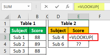
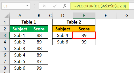
#1 VLOOKUP Function to Fetch Data
The data in multiple sheets are common in many offices, but fetching the data from one worksheet to another and from one workbook to another is a challenge for beginners in Excel.
In table 1, we have the subject list and their respective scores, and in table 2, we have some subject names, but we do not have scores for them. So, using these subject names in table 2, we need to fetch the data from table 1.
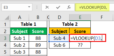
- First, let us open the VLOOKUP function in the E2 cell.
Then, select the LOOKUP value as a D3 cell.
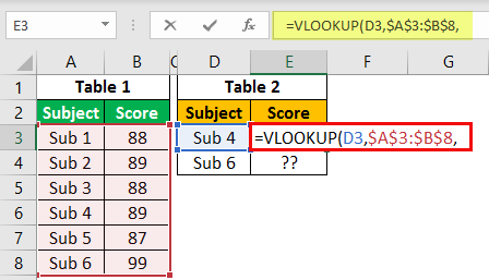
Next, we must select the table array as A3 to B8 and press the F4 key to make them an absolute reference.
Column Index Number is from the selected table array from which column you need to fetch the data. So, in this case, from the second column, we need to bring the data.
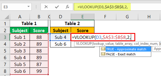
For the last argument range, LOOKUP, we must select FALSE as the option, or else we can enter.

Close the bracket and press the Enter key to get the score of Sub 4. Also, copy the formula and paste it to the below cell.
You have learned a formula to fetch values from different tables based on a LOOKUP value.
#2 IF Condition to Do Logical Test
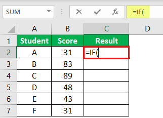
The Excel IF condition can be your friend in many situations because of its ability to conduct logical tests. For example, assume you want to test the scores of students and give the result. Below is the data for your reference.

In the above table, we have students’ scores from the examination. So we need to arrive at the result as either “PASS” or “FAIL” based on these scores. So to reach these results criteria, if the score is >=35, the result should be “PASS” or else “FAIL.”
- We must first open the IF condition in the C2 cell.
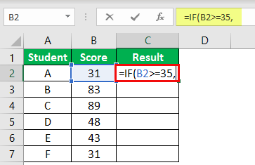
- The first argument is logical to test.So, in this example, we need to do the logical test of whether the score is >=35, select the score cell B2, and apply the logical test as B2 >= 35.
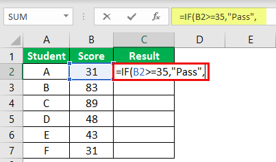
- The next argument is value if true. If the applied logical test is “TRUE,” what is the value we need? If the logical test is “TRUE,” we need the result as “Pass.”
- So, the final part is value if false.If the applied logical test is “FALSE,” then we need the result as “Fail.”
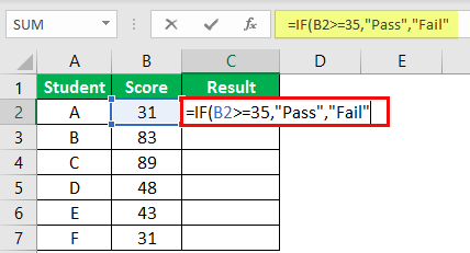
- Now, close the bracket, and we also need to fill the formula to the remaining cells.
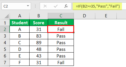
So, students A and F scored less than 35. Therefore, the result has arrived as “FAIL.”
#3 CONCATENATE Function to Combine Two or More Values

- First, we need to open the CONCATENATE function in the C2 cell.
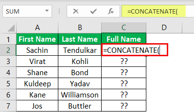
- For the first argument, “Text 1,“ select the “First Name” cell, and for “Text 2,” choose the “Last Name” cell.
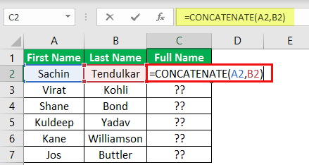
- Then, we need to apply the formula to all the cells to get the full name.

- If you want space as the “First Name” and “Last Name” separator, we can use the space character in double-quotes after selecting the first name.
#4 Count Only Numerical Values
If we want to count only numerical values from the range, you need to use the COUNT function in Excel. Take a look at the below data.
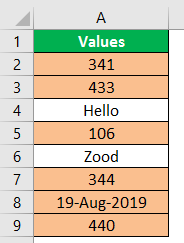
From the above table, we need to count only numerical values. For this, we can use the COUNT function.
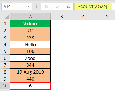
The result of the COUNT function is 6. The total count of cells is 8, but we have got the count of numerical values as 6. In cells A4 and A6, we have text values, but in cell A8, we have date values. The Excel COUNT function treats the date also as a numerical value only.
Note: “Date” and “Time” values are numerical values if the formatting is correct. Otherwise, they will be treated as “text” values.
#5 Count All Values

We got the count as 8 because the COUNTA function has counted all the cell values.
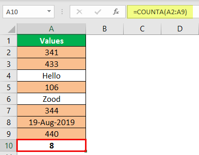
Note: Both the COUNT and COUNTA functions ignore blank cells.
#6 Count Based on Condition
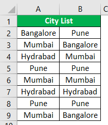
From this “City List,” if we want to count how many times “Bangalore” city is mentioned, we must open the COUNTIF function.

The first argument is “RANGE,” so we need to select the range of values from A2 to B9.
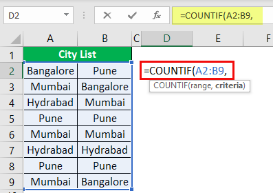
The second argument is “Criteria,” i.e., what you want to count, i.e., “Bangalore.
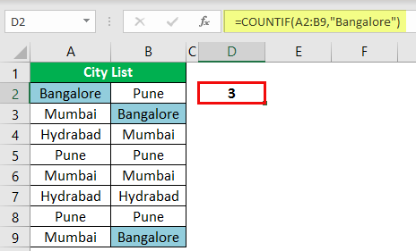
Bangalore has appeared three times in the range A2 to B9, so the COUNTIF function returns 3 as the count.
#7 Count Number of Characters in the Cell
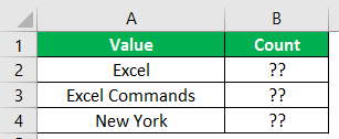
“Excel” has 5 characters, so the result is 5.
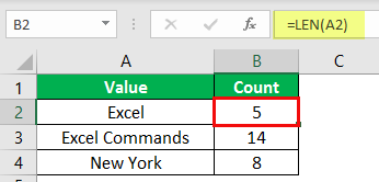
Note: Space is also considered as one character.
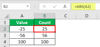
#8 Convert Negative Value to Positive Value
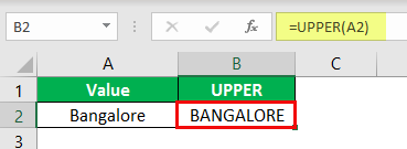
#9 Convert All Characters to UPPERCASE Values
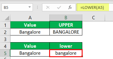
And if we want to convert all the text values to LOWERCASE values, then use the LOWER formula.
#10 Find Maximum and Minimum Values

Things to Remember
- These are some of the important formulas/commands in excel which are used regularly.
- We can also use these functions at the advanced level.
- There are more advanced formulas in Excel which come under advanced level courses.
- Space is considered one character.
Recommended Articles
This article is a guide to Excel Commands. Here, we discuss the top 10 commands in Excel, examples, and a downloadable template. You may learn more about Excel from the following articles: –
Источник

- VBA ЕСЛИ НЕ
VBA ЕСЛИ НЕ
На любом языке программирования у нас есть логические операторы И ИЛИ и НЕ. У каждого оператора есть определенная функция. AND объединяет два или более операторов и возвращает значения true, если каждое из утверждений истинно, где находится в операторе OR, если любое из утверждений истинно, значение истинно. Оператор НЕ — это другое. Оператор NOT отрицает данное утверждение. Мы используем эти логические операторы с операторами IF в нашем повседневном анализе данных. Если мы используем оператор IF NOT в VBA, рассмотрим это как обратную функцию.
Выше мы обсуждали, что мы используем логические операторы с операторами if. В этой статье мы будем использовать оператор NOT с оператором if. Ранее я говорил, что оператор IF NOT в VBA также рассматривается как обратная функция. Почему, потому что, если условие истинно, оно возвращает ложь, а если условие ложно, оно возвращает истину. Посмотрите ниже,
ЕСЛИ A> B равно IF НЕ B> A
Оба предложения if выше идентичны, как? В первом операторе, если A больше, чем B, выполняется следующий оператор, а в следующем, если не оператор, означает, что B не больше, чем A, что само по себе означает, что A больше, чем B.
Самый простой способ понять утверждение IF NOT должно быть следующим:
Если верно, то если не ложно, то
Или мы можем сказать, что
Если Ложь, тогда ЕСЛИ НЕ Верно
Оба утверждения в Сравнении 1 и Сравнении 2 идентичны друг другу.
Давайте использовать функцию IF NOT в нескольких примерах, которые сделают ее более понятной для нас.
Примечание : мы должны помнить, что для использования VBA в Excel мы должны сначала включить вкладку нашего разработчика на вкладке файлов, а затем в разделе параметров.
Как использовать Excel VBA, если нет?
Мы научимся использовать VBA IF Not с несколькими примерами в Excel.
Вы можете скачать этот VBA, если не шаблон Excel здесь — VBA, если не шаблон Excel
Пример № 1 — VBA, если нет
Выполните следующие шаги, чтобы использовать ЕСЛИ НЕ в Excel VBA.
Например, у меня есть два значения на листе 1 в ячейках A1 и B1. Посмотрите на них ниже,
То, что я хочу сделать, это сравнить эти два значения, которое больше, используя оператор IF NOT в VBA.
Шаг 1: Перейдите на вкладку разработчика и нажмите Visual Basic, чтобы открыть редактор VB.
Шаг 2: Вставьте модуль из вкладки вставки в VB Editor. Дважды щелкните по модулю, который мы только что вставили, чтобы открыть другое окно, в которое мы собираемся написать наш код.
Шаг 3: Каждый код VBA начинается с подфункции, как показано ниже,
Код:
Sub Sample () End Sub

Шаг 4: Объявите две переменные как целые числа, которые будут хранить наши значения из ячеек A1 и B1.
Код:
Sub Sample () Dim A, B As Integer End Sub

Шаг 5: Чтобы присвоить значения этим переменным, нам нужно сначала активировать лист с помощью следующего кода.
Код:
Sub Sample () Dim A, B As Integer Worksheets ("Sheet1"). Активировать End Sub
Шаг 6: Теперь мы присвоим этим переменным значения A1 и B1.
Код:
Sub Sample () Dim A, B As Integer Worksheets ("Sheet1"). Активировать A = Range ("A1") B = Range ("B1") End Sub
Шаг 7: Давайте сравним обе переменные, используя оператор IF NOT с помощью следующего кода:
Код:
Sub Sample () Dim A, B As Integer Worksheets ("Sheet1"). Активируйте A = Range ("A1") B = Range ("B1") Если не A> B, то MsgBox "B больше, чем A" Иначе MsgBox «A больше, чем B» End If End Sub
Шаг 8: Запустите приведенный выше код с кнопки запуска в VBA, или мы можем нажать кнопку F5, чтобы сделать то же самое. Мы получим следующий результат.

Шаг 9: Давайте инвертируем значения A и B и снова запустим код, чтобы увидеть следующий результат.
В первом выполнении A было больше, чем B, но мы сравнивали IF NOT A> B, изначально условие было истинным, поэтому оно отображало результат для оператора False, т. Е. A больше, чем B, и наоборот для второго выполнения.
Пример № 2 — VBA, если нет
В первом примере мы сравнили целые числа, давайте сравним строки в этом примере с оператором IF NOT в VBA. В том же листе 1 у нас есть две строки в ячейках A3 и B3 следующим образом:
Давайте сравним обе строки, используя оператор IF NOT.
Шаг 1: Чтобы открыть VB Editor, сначала нажмите вкладку разработчика, а затем нажмите Visual Basic.
Шаг 2: В тот же модуль, который мы вставили выше, дважды щелкните по нему, чтобы начать писать второй код.

Шаг 3: Объявите подфункцию под кодом, который мы написали первым.
Код:
Sub Sample1 () End Sub
Шаг 4: Объявите две переменные в виде строки, в которой будут храниться наши значения из ячеек A3 и B3.
Код:
Sub Sample1 () Dim A, B As String End Sub
Шаг 5: Чтобы присвоить значения этим переменным, нам нужно сначала активировать лист с помощью следующего кода, чтобы использовать его свойства.
Код:
Sub Sample1 () Dim A, B As String Worksheets ("Sheet1"). Активировать End Sub
Шаг 6: Теперь мы присвоим этим переменным значения A3 и B3.
Код:
Sub Sample1 () Dim A, B As String Worksheet ("Sheet1"). Активировать A = диапазон ("A3") B = диапазон ("B3") End Sub
Шаг 7: Давайте сравним обе переменные, используя оператор IF NOT, начав оператор if следующим образом:
Код:
Sub Sample1 () Dim A, B As String Worksheets ("Sheet1"). Активируйте A = Range ("A3") B = Range ("B3"), если не A = B, тогда End Sub
Шаг 8: Если условие A = B является истинным, то приведенное выше утверждение отрицает его и возвращает значение как ложное.
Код:
Sub Sample1 () Dim A, B As String Worksheets ("Sheet1"). Активируйте A = Range ("A3") B = Range ("B3") Если не A = B, то MsgBox "Обе строки не совпадают" Конец Sub

Шаг 9: Если обе строки одинаковы, т. Е. Если результат возвращен как true, отобразите следующее сообщение,
Код:
Sub Sample1 () Dim A, B As String Worksheets ("Sheet1"). Активируйте A = Range ("A3") B = Range ("B3") Если не A = B, то MsgBox "Обе строки не одинаковы" Иначе MsgBox "Обе строки одинаковы" End If End Sub
Шаг 10: Теперь давайте запустим приведенный выше код, нажав кнопку F5 или указанную кнопку запуска. Запустив код, мы получим следующий результат.
Шаг 11: Теперь давайте сделаем одинаковые строки в ячейках A3 и B3, чтобы увидеть разные результаты при выполнении одного и того же кода.

В первом исполнении A не было похоже на B, но мы сравнивали IF NOT A = B, изначально условие было истинным, поэтому оно отображало результат для ложного утверждения, т. Е. Обе строки не совпадают, и когда обе строки были одинаковыми, мы получаем разные сообщения, так как обе строки одинаковы.
То, что нужно запомнить
- ЕСЛИ НЕ является сравнительным утверждением.
- Если NOT отрицает значение условия, то есть если условие истинно, оно возвращает ложь, и наоборот.
- Если оператор NOT является в основном обратной функцией.
Рекомендуемые статьи
Это было руководство для VBA, если нет. Здесь мы обсудили, как использовать Excel VBA If Not вместе с практическими примерами и загружаемым шаблоном Excel. Вы также можете просмотреть наши другие предлагаемые статьи —
- Работа с VBA Active Cell
- Удаление строки в VBA
- Как использовать Excel VBA Transpose?
- Как исправить ошибку 1004 с помощью VBA
- VBA не

Logical functions are some of the most popular and useful in Excel. They can test values in other cells and perform actions dependent upon the result of the test. This helps us to automate tasks in our spreadsheets.
How to Use the IF Function
The IF function is the main logical function in Excel and is, therefore, the one to understand first. It will appear numerous times throughout this article.
Let’s have a look at the structure of the IF function, and then see some examples of its use.
The IF function accepts 3 bits of information:
=IF(logical_test, [value_if_true], [value_if_false])
- logical_test: This is the condition for the function to check.
- value_if_true: The action to perform if the condition is met, or is true.
- value_if_false: The action to perform if the condition is not met, or is false.
Comparison Operators to Use with Logical Functions
When performing the logical test with cell values, you need to be familiar with the comparison operators. You can see a breakdown of these in the table below.

Now let’s look at some examples of it in action.
IF Function Example 1: Text Values
In this example, we want to test if a cell is equal to a specific phrase. The IF function is not case-sensitive so does not take upper and lower case letters into account.
The following formula is used in column C to display “No” if column B contains the text “Completed” and “Yes” if it contains anything else.
=IF(B2="Completed","No","Yes")
Although the IF function is not case sensitive, the text must be an exact match.
IF Function Example 2: Numeric Values
The IF function is also great for comparing numeric values.
In the formula below we test if cell B2 contains a number greater than or equal to 75. If it does, then we display the word “Pass,” and if not the word “Fail.”
=IF(B2>=75,"Pass","Fail")
The IF function is a lot more than just displaying different text on the result of a test. We can also use it to run different calculations.
In this example, we want to give a 10% discount if the customer spends a certain amount of money. We will use £3,000 as an example.
=IF(B2>=3000,B2*90%,B2)
The B2*90% part of the formula is a way that you can subtract 10% from the value in cell B2. There are many ways of doing this.
What’s important is that you can use any formula in the value_if_true or value_if_false sections. And running different formulas dependent upon the values of other cells is a very powerful skill to have.
IF Function Example 3: Date Values
In this third example, we use the IF function to track a list of due dates. We want to display the word “Overdue” if the date in column B is in the past. But if the date is in the future, calculate the number of days until the due date.
The formula below is used in column C. We check if the due date in cell B2 is less than today’s date (The TODAY function returns today’s date from the computer’s clock).
=IF(B2<TODAY(),"Overdue",B2-TODAY())
What are Nested IF Formulas?
You may have heard of the term nested IFs before. This means that we can write an IF function within another IF function. We may want to do this if we have more than two actions to perform.
One IF function is capable of performing two actions (the value_if_true and value_if_false ). But if we embed (or nest) another IF function in the value_if_false section, then we can perform another action.
Take this example where we want to display the word “Excellent” if the value in cell B2 is greater than or equal to 90, display “Good” if the value is greater than or equal to 75, and display “Poor” if anything else.
=IF(B2>=90,"Excellent",IF(B2>=75,"Good","Poor"))
We have now extended our formula to beyond what just one IF function can do. And you can nest more IF functions if necessary.
Notice the two closing brackets on the end of the formula—one for each IF function.
There are alternative formulas that can be cleaner than this nested IF approach. One very useful alternative is the SWITCH function in Excel.
The AND and OR functions are used when you want to perform more than one comparison in your formula. The IF function alone can only handle one condition, or comparison.
Take an example where we discount a value by 10% dependent upon the amount a customer spends and how many years they have been a customer.
On their own, the AND and OR functions will return the value of TRUE or FALSE.
The AND function returns TRUE only if every condition is met, and otherwise returns FALSE. The OR function returns TRUE if one or all of the conditions are met, and returns FALSE only if no conditions are met.
These functions can test up to 255 conditions, so are certainly not limited to just two conditions like is demonstrated here.
Below is the structure of the AND and OR functions. They are written the same. Just substitute the name AND for OR. It is just their logic which is different.
=AND(logical1, [logical2] ...)
Let’s see an example of both of them evaluating two conditions.
AND Function example
The AND function is used below to test if the customer spends at least £3,000 and has been a customer for at least three years.
=AND(B2>=3000,C2>=3)
You can see that it returns FALSE for Matt and Terry because although they both meet one of the criteria, they need to meet both with the AND function.
OR Function Example
The OR function is used below to test if the customer spends at least £3,000 or has been a customer for at least three years.
=OR(B2>=3000,C2>=3)
In this example, the formula returns TRUE for Matt and Terry. Only Julie and Gillian fail both conditions and return the value of FALSE.
Using AND and OR with the IF Function
Because the AND and OR functions return the value of TRUE or FALSE when used alone, it’s rare to use them by themselves.
Instead, you’ll typically use them with the IF function, or within an Excel feature such as Conditional Formatting or Data Validation to perform some retrospective action if the formula evaluates to TRUE.
In the formula below, the AND function is nested inside the IF function’s logical test. If the AND function returns TRUE then 10% is discounted from the amount in column B; otherwise, no discount is given and the value in column B is repeated in column D.
=IF(AND(B2>=3000,C2>=3),B2*90%,B2)
The XOR Function
In addition to the OR function, there is also an exclusive OR function. This is called the XOR function. The XOR function was introduced with the Excel 2013 version.
This function can take some effort to understand, so a practical example is shown.
The structure of the XOR function is the same as the OR function.
=XOR(logical1, [logical2] ...)
When evaluating just two conditions the XOR function returns:
- TRUE if either condition evaluates to TRUE.
- FALSE if both conditions are TRUE, or neither condition is TRUE.
This differs from the OR function because that would return TRUE if both conditions were TRUE.
This function gets a little more confusing when more conditions are added. Then the XOR function returns:
- TRUE if an odd number of conditions return TRUE.
- FALSE if an even number of conditions result in TRUE, or if all conditions are FALSE.
Let’s look at a simple example of the XOR function.
In this example, sales are split over two halves of the year. If a salesperson sells £3,000 or more in both halves then they are assigned Gold standard. This is achieved with an AND function with IF like earlier in the article.
But if they sell £3,000 or more in either half then we want to assign them Silver status. If they don’t sell £3,000 or more in both then nothing.
The XOR function is perfect for this logic. The formula below is entered into column E and shows the XOR function with IF to display “Yes” or “No” only if either condition is met.
=IF(XOR(B2>=3000,C2>=3000),"Yes","No")
The NOT Function
The final logical function to discuss in this article is the NOT function, and we have left the simplest for last. Although sometimes it can be hard to see the ‘real world’ uses of the function at first.
The NOT function reverses the value of its argument. So if the logical value is TRUE, then it returns FALSE. And if the logical value is FALSE, it will return TRUE.
This will be easier to explain with some examples.
The structure of the NOT function is;
=NOT(logical)
NOT Function Example 1
In this example, imagine we have a head office in London and then many other regional sites. We want to display the word “Yes” if the site is anything except London, and “No” if it is London.
The NOT function has been nested in the logical test of the IF function below to reverse the TRUE result.
=IF(NOT(B2="London"),"Yes","No")
This can also be achieved by using the NOT logical operator of <>. Below is an example.
=IF(B2<>"London","Yes","No")
NOT Function Example 2
The NOT function is useful when working with information functions in Excel. These are a group of functions in Excel that check something, and return TRUE if the check is a success, and FALSE if it is not.
For example, the ISTEXT function will check if a cell contains text and return TRUE if it does and FALSE if it does not. The NOT function is helpful because it can reverse the result of these functions.
In the example below, we want to pay a salesperson 5% of the amount they upsell. But if they did not upsell anything, the word “None” is in the cell and this will produce an error in the formula.
The ISTEXT function is used to check for the presence of text. This returns TRUE if there is text, so the NOT function reverses this to FALSE. And the IF performs its calculation.
=IF(NOT(ISTEXT(B2)),B2*5%,0)
Mastering logical functions will give you a big advantage as an Excel user. To be able to test and compare values in cells and perform different actions based on those results is very useful.
This article has covered the best logical functions used today. Recent versions of Excel have seen the introduction of more functions added to this library, such as the XOR function mentioned in this article. Keeping up to date with these new additions will keep you ahead of the crowd.
READ NEXT
- › How to Find the Function You Need in Microsoft Excel
- › Functions vs. Formulas in Microsoft Excel: What’s the Difference?
- › How to Group Worksheets in Excel
- › How to Use the IF Function in Microsoft Excel
- › How to Use the IFS Function in Microsoft Excel
- › How to Use an Advanced Filter in Microsoft Excel
- › How to Use the IS Functions in Microsoft Excel
- › The New NVIDIA GeForce RTX 4070 Is Like an RTX 3080 for $599
Purpose
Reverse arguments or results
Usage notes
The NOT function returns the opposite of a given logical or Boolean value. Use the NOT function to reverse a Boolean value or the result of a logical expression.
- When given FALSE, NOT returns TRUE.
- When given TRUE, NOT returns FALSE.
Example #1 — not green or red
In the example shown, the formula in C5, copied down, is:
=NOT(OR(B5="green",B5="red"))
The literal translation of this formula is «NOT green or red». At each row, the formula returns TRUE if the color in column B is not green or red, and FALSE if the color is green or red.
Example #2 — Not blank
A common use case for the NOT function is to reverse the behavior of another function. For example, If cell A1 is blank (empty), the ISBLANK function will return TRUE:
=ISBLANK(A1) // TRUE if A1 is empty
To reverse this behavior, wrap the NOT function around the ISBLANK function:
=NOT(ISBLANK(A1)) // TRUE if A1 is NOT empty
By adding NOT the output from ISBLANK is reversed. This formula will return TRUE when A1 is not empty and FALSE when A1 is empty. You might use this kind of test to only run a calculation if there is a value in A1:
=IF(NOT(ISBLANK(A1)),B1/A1,"")
Translation: if A1 is not blank, divide B1 by A1, otherwise return an empty string («»). This is an example of nesting one function inside another.