
Excel for Microsoft 365 Excel for Microsoft 365 for Mac Excel for the web Excel 2021 Excel 2021 for Mac Excel 2019 Excel 2019 for Mac Excel 2016 Excel 2016 for Mac Excel 2013 Excel 2010 Excel 2007 Excel for Mac 2011 Excel Starter 2010 More…Less
This article describes the formula syntax and usage of the MID and MIDB function in Microsoft Excel.
Description
MID returns a specific number of characters from a text string, starting at the position you specify, based on the number of characters you specify.
MIDB returns a specific number of characters from a text string, starting at the position you specify, based on the number of bytes you specify.
Important:
-
These functions may not be available in all languages.
-
MID is intended for use with languages that use the single-byte character set (SBCS), whereas MIDB is intended for use with languages that use the double-byte character set (DBCS). The default language setting on your computer affects the return value in the following way:
-
MID always counts each character, whether single-byte or double-byte, as 1, no matter what the default language setting is.
-
MIDB counts each double-byte character as 2 when you have enabled the editing of a language that supports DBCS and then set it as the default language. Otherwise, MIDB counts each character as 1.
The languages that support DBCS include Japanese, Chinese (Simplified), Chinese (Traditional), and Korean.
Syntax
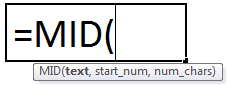
MID(text, start_num, num_chars)
MIDB(text, start_num, num_bytes)
The MID and MIDB function syntax has the following arguments:
-
Text Required. The text string containing the characters you want to extract.
-
Start_num Required. The position of the first character you want to extract in text. The first character in text has start_num 1, and so on.
-
If start_num is greater than the length of text, MID/MIDB returns «» (empty text).
-
If start_num is less than the length of text, but start_num plus num_chars exceeds the length of text, MID/MIDB returns the characters up to the end of text.
-
If start_num is less than 1, MID/MIDB returns the #VALUE! error value.
-
-
Num_chars Required for MID. Specifies the number of characters you want MID to return from text.
-
If num_chars is negative, MID returns the #VALUE! error value.
-
-
Num_bytes Required for MIDB. Specifies the number of characters you want MIDB to return from text, in bytes.
-
If num_bytes is negative, MIDB returns the #VALUE! error value.
-
Example
Copy the example data in the following table, and paste it in cell A1 of a new Excel worksheet. For formulas to show results, select them, press F2, and then press Enter. If you need to, you can adjust the column widths to see all the data.
|
Data |
||
|
Fluid Flow |
||
|
Formula |
Description |
Result |
|
=MID(A2,1,5) |
Returns 5 characters from the string in A2, starting at the 1st character. |
Fluid |
|
=MID(A2,7,20) |
Returns 20 characters from the string in A2, starting at the 7th character. Because the number of characters to return (20) is greater than the length of the string (10), all characters, beginning with the 7th, are returned. No empty characters (spaces) are added to the end. |
Flow |
|
=MID(A2,20,5) |
Because the starting point is greater than the length (10) of the string, empty text is returned. |
Need more help?

Joe4
MrExcel MVP, Junior Admin
-
#2
Welcome to the Board!
You can imbed up to 7 levels in an IF statement. Your IF would look something like:
=IF(MID(B2,4,1)=5,5,IF(MID(B2,4,1)=1,1.75,…))
If you have more than that, take a look at using something like VLOOKUP (Excel’s built-in help on functions has details and example of that).
I have also seen some people using some other clever methods using arrays, though that quite isn’t my specialty!
-
#3
Welcome to the board.
Sure it’s possible, but judging by your description, I wouldn’t use IF..
It looks like you have more than 2 options for value to return based on what the 4th character is. I would use a lookup.
=LOOKUP(MID(B2,4,1)+0,{1,5},{1.75,5})
It takes the 4th character of B2 (the +0 makes it a number isntead of a text string).
Finds that number in the first array {1,5}
Returns the corresponding value from the 2nd array {1.75,5}
Make sure the 1st array is listed in ASCENDING order, smallest to largest from left to right.
Hope that helps..
Joe4
MrExcel MVP, Junior Admin
-
#4
There it is. That was the method I was thinking about. Thanks Jon.
-
#5
That woked perfect! Thanks for the quick reply from you both!
-
#6
Also, the lookup may need some tweeking / error handling.
As the formula is, it will error if the 4th character is NOT a number, OR if there IS no 4th character, like the string is only 2 or 3 characters long..
Also, if say the 4th character is a 3 (which is NOT in the lookup array), it will return the closest match (largest # that is less than or equal to the lookup). So in this case it will return as if the 4th character was a 1.
all this can be adjusted for if you need it. Probably more like an Index/Match type of formula
-
#7
Is there a way to have the value return » » empty if the first field is empty. It shows #value now if the field is empty. Not a big deal, just trying to clean it up. Thanks again.
-
#8
Sure, but it might be better to test if the Length of B2 is less than 4 (because that will cause error as well).
=IF(LEN(B2)<4,»»,LOOKUP(MID(B2,4,1)+0,{1,5},{1.75,5}))
-
#9
Also, the lookup may need some tweeking / error handling.
As the formula is, it will error if the 4th character is NOT a number, OR if there IS no 4th character, like the string is only 2 or 3 characters long..
Also, if say the 4th character is a 3 (which is NOT in the lookup array), it will return the closest match (largest # that is less than or equal to the lookup). So in this case it will return as if the 4th character was a 1.
all this can be adjusted for if you need it. Probably more like an Index/Match type of formula
I was hoping to avoid this by formating the cell to limit it to the number of characters that I need (00-0000)
-
#10
That got it. Thanks again, you guy’s are FAST!
The MID function returns a specific number of characters from the middle of the string after we state the starting position and the number of characters to extract. The MID Function in Excel is one of the text functions that allows us to get a substring from a stringtext as per our requirement
It is one of the most useful functions when we want to extract the middle name from the full name, the domain name from email IDs, or any substring between two characters.

Syntax
The syntax of the MID function is as follows:
=MID(text,start_num,num_chars)
The MID function in Excel accepts three arguments and all three arguments are mandatory.
Arguments:
‘text‘ – This holds the value of the input text/string. A cell reference containing the input string or text enclosed in double quotes are both acceptable input values.
‘start_num‘ – The position of the first character we want to extract. It must be an integer/formula which indicates the starting position of the extraction.
‘num_chars‘ – Number of characters we wish to extract from the starting point. The num_chars argument indicates the character length of the return value.
Important Characteristics of the MID Function
One of the essential and basic characteristics of the MID function being a text function is that it always returns a text value regardless of the input value. Even if the retrieved substring is only made up of numbers, it will be in text format. Other important MID function features are as follows:
- If the value of start_num exceeds the length of input text, the MID function returns «» (empty text).
- If the start_num value is less than 1, the function returns a #VALUE! error.
- If the value of num_chars is a negative number, the MID function gives a #VALUE error.
- If the num_chars value is less than 1, then the MID function’s return value is an empty string, a blank cell.
Last of all, if the sum of the value of start_num and num_chars is greater than the total input text length, the MID function returns all the characters from start_num to the last character. This characteristic comes in very handy for certain conditions. We will find out in the examples below.
Examples of MID Function
The MID function can be used independently or can be combined with various other Excel functions such as SEARCH, FIND, LEN, and more. Let’s go through some examples to fully comprehend the usage and utility of the MID function.
Example 1: Basic Functionality of the MID Function
In the below example, we have taken 3 different instances and tried using the basic MID function.

In the first case, the input text/string is a full name ‘Cassie Martha Soros’ where we wish to extract the middle name –»Martha». So, using the MID function we apply the formula:
=MID(B3,8,6)
Here, the first parameter text is the cell reference B3. The second parameter start_num is the starting position which is 8 as the first name is 6 characters long, the space is the 7th character and then we add 1 so that we reach the beginning of the middle name. Lastly, the third argument num_chars is the number of characters of the middle name which is 6.
The second instance is where we are trying to extract the house number and street address from the complete address in cell B4. We are checking if the MID function counts a special character (,) and also whether the MID function can return characters from the beginning of the text or only from the middle. The formula goes as follows:
=MID(B4,1,13)
The first parameter is B4, the input text. The second parameter is 1 as the house number is in the beginning. Finally, the third parameter is 13 which is the house number (3 characters long) combined with a comma, a space character, and then the street name which is 8 characters long. Hence our output, in this case, becomes ‘220, Kisvagen’.
In the last example, the input text is in cell B5, which is actually a number 123456789. To extract 4 digits from the second position, the formula would be:
=MID(B5,2,4)
Here, the output value is left aligned. Is it a text value? We have something to learn here, which we will find in the section below.
Example 2: Extract Substring After a Specific Character
In the following example, we are trying to extract a substring from the input text after a special character. The dataset in column B in this example consists of Employee IDs; a combination of the department name, and a unique ID followed by the employee’s date of birth.
For instance, in the Employee ID TECH-1234-08051990, the employee belongs to the tech team, the unique ID is 1234, and the date of birth is 08 May 1990.
We want to extract the unique ID from each Employee ID. Using the MID function, we can extract it from the input string, but the issue is that the character length of the department name varies. Resultantly, the value of start_num varies.

Lucky for us, the department name is followed by a hyphen ‘-‘, and the employee ID is 4 characters long. Now, we can use the MID function combined with the FIND function. The FIND function will locate the hyphen’s ‘-‘ position, which will be the input value of start_num.
Use the FIND function as follows:
=FIND("-",B3)
This formula locates the hyphen in B3 and returns 4 (the hyphen is the 4th character in B3). To use the FIND function as an input value for the start_num parameter, we must add 1 to this result because the unique ID begins from the 5th character of the text string and we don’t want to see the hyphen in the final result.
The value of num_chars shall be 4 as all the unique IDs in our example are 4-digit numbers. So, combining the FIND and MID functions, the final function is as follows:
=MID(B3,FIND("-",B3)+1,4)
And here’s how this formula extracts the unique IDs for us:

Example 3: Extract First or Last Name
Imagine we have a data set of peoples’ names and are asked to extract first, middle and last names in different columns. Usually, we would want to use the LEFT function for the first name and the RIGHT function for the last name. However, the functionality of two different functions can be accomplished using the MID function alone.
Let’s learn how to extract first and last names using the MID function. We cannot simply use the MID function as the starting position for separating last names as the number of characters will vary for each name. Ergo, we will use the SEARCH function to our advantage and then merge it with the MID function.
We could have used the earlier mentioned FIND function too, but as we have understood the functionality of the FIND function, let’s try to learn the MID function with the SEARCH function here. Also, the SEARCH function is case insensitive and that will make our task even easier.
Extract First Name using MID Function
The first and last names are divided by a space, a common pattern we can make use of. The beginning position in the MID function will be the starting of the string, whereas the number of characters can be determined using the SEARCH function.
The position of the space » » is where the first name ends and hence, is the number of characters to be extracted. The space character is located in the name using the SEARCH function, which returns its position, from which we deduct 1 to delete the inclusion of the extra space.
Let’s try to put this logic in the form of an Excel formula.
Seeing the example ahead, the first name in cell B3 is ‘Simon Rogers’. If we used the MID function only on this cell, we would try:
=MID(B3,1,5)
However, this formula will not give us the required result for all other cells since all the names won’t be 5 letters.
Let’s generalize it so we can use it for the complete dataset.

As the first parameter, start_num remains the same for all the names,. To determine the second parameter, we must find the position of the space. To find the position of the space » » using the SEARCH function, the formula will go as follows:
=SEARCH(" ",B3)
Combining it with the MID function, the formula will become:
=MID(B3,1,SEARCH(" ",B3))
To remove the extra trailing space, subtract 1 from the position. The final formula will be:
=MID(B3,1,SEARCH(" ",B3)-1)

Furthermore, can we use the same logic to extract the last name? Let’s find out.
Extract Last Name using MID Function
To pull out the last name using the MID function, we can use the SEARCH function to point out the start_num parameter as the last name begins after the space. How to find the number of characters (num_chars) to extract?
As mentioned earlier, if the total of the start_num and num_chars is more than the length of the string, the MID function returns the remaining string from the start_num. So, utilizing that to our advantage, there are two ways to use the MID function.
The first one is fairly simple. Assuming that the total character length of names will never exceed 1000, we can assign 1000 to the num_chars parameter.
The SEARCH function will determine the position of the space » » using the formula:
=SEARCH(" ",B3)
This will be the input value of the first parameter start_num. Assigning 1000 to the second parameter, the formula will become:
=MID(B3,SEARCH(" ",B3),1000)

To remove the extra leading spaces from the extracted last names, use the TRIM function. The final MID function will be used as follows:
=TRIM(MID(B3,SEARCH(" ",B3),1000))
Now we have the last names extracted by the MID and SEARCH functions and leading spaces removed by the TRIM function:

The second way is more elegant. Instead of an assumed number in the num_chars parameter, we can use the LEN function to determine the total length of the name and use that value in the num_chars parameter.
Combining the LEN & SEARCH functions with the MID function, the formula will be as follows:
=MID(B3,SEARCH(" ",B3),LEN(B3))
Here, LEN function will return the total length of the input string, and SEARCH function will extract the position of the space » » in the string. The ultimate effect is similar to what we have seen in the previous formula. The location of the space character added to the total characters of B3 will obviously be more than the total characters in B3.

To polish it further, we can use the TRIM function to eliminate all the extra spaces.
=TRIM(MID(B3,SEARCH(" ",B3),LEN(B3)))

Substring Between Two Delimiters
After practicing the above examples, we can extract a substring from a string after determining the position of the space » » or any other special character. Now, what if the input string is long with several delimiters? Just for clarity, one or more characters that divide text strings are known as delimiters, such as space ( ), quotes («), commas (,), semicolons (;), slashes (/) or pipes (|).
When we dive in further, there are two scenarios of extracting a substring from an input string between delimiters; first when they are different and second when the delimiters are the same. Let’s understand both cases using an example.
Example 1 – Extracting Substring Between Two Different Delimiters
Let’s assume we have a set of email IDs, and for research purposes, we want to extract the domain name from each email ID to analyze which one is most preferred. The email ID structure goes as follows ‘[email protected]’, where ‘learning’ is a username and gmail is a domain name.

As we can see, we have two different delimiters (@) and (.) separating the domain name (gmail) from the rest of the string (username). So, to pull out the substring, we must locate the position of two delimiters where the first delimiter is the starting position (start_num), and using the second delimiter, we can calculate the number of characters to be extracted.
As we already know, the MID function consists of three arguments. The first argument is the cell reference to email ID (B3). The second argument is the starting position which can be calculated using the SEARCH function:
=SEARCH("@",B3)
This formula will give us the position of the first delimiter (@). As we require the starting position to be one character after (@), we add 1.
Lastly, for the third argument (num_chars), we need the number of characters to be extracted. We can find the location of the second delimiter (.) and then subtract the position of the first delimiter. The formula goes as follows:
=SEARCH(".",B3)-SEARCH("@",B3)
To finalize and remove the trailing space, subtract 1.
Putting it all together, the final MID function formula to extract the substring from two different characters is:
=MID(B3,SEARCH("@",B3)+1,(SEARCH(".",B3)-SEARCH("@",B3))-1)
This is how our experiment turned out:

Example 2: Extracting Substring Between Same Delimiters
In the above examples, we already know how to extract the first and last name from the full name using the MID function. However, what about the middle name? We cannot simply use the basic MID function as the character length of middle names varies for each person.
However, in the previous example, we learned how to extract a substring between two delimiters.
As we will notice, there is a space ( ) before and after the middle name, separating it from the first & last name. We can find the position of two delimiters (in this case, both the delimiters are space characters) and extract the middle name from the full name.
In the given dataset in column B, we have the list of full names. Let’s take the example of the first name in cell B3.

The first parameter of the MID function is the input text which is cell B3. For the second parameter, that is start_num, if we find the position of the space before the middle name and then add 1 to it, we should have our argument input. Using the SEARCH function, the position of the first space » » can be determined using the following formula:
=SEARCH(" ",B3)+1
This returns 7 and if we do a quick count check, indeed the middle name’s first letter is the 7th character of the text string.
Easy enough, right?
Now, to determine the number of characters to be returned, we can find the position of the second space » » (after the middle name) and subtract the position of the first space from it.
Remember, the SEARCH function has an additional third optional parameter start_num stating the starting position of the search within the string. This will come in handy here as there are two spaces in this text (full name). To find the position of the second space, the formula goes as follows:
=SEARCH(" ",B3,(SEARCH(" ",B3)+1)
Explaining further, we are telling the SEARCH function to find » » in B3 starting after the position of the first space. If we don’t use the nested SEARCH function, it will keep returning the position of the first space, and we don’t want that, do we?
This formula returns 11 which you can tally again. Now that we have the position of both the space characters 11-7 is the number of characters to extract. Combining all to finish our MID function, the formula goes as follows:
=MID(B3,SEARCH(" ",B3)+1,SEARCH(" ",B3,(SEARCH(" ",B3)+1))-(SEARCH(" ",B3)+1))
The MID function will return 4 characters from B3 starting from the character after the first space. The result is Dona and the rest can be seen below:

Forcing MID Function to Return Numbers
Like other text functions in Excel, the output value of the MID function is always in text format. Even if the input or output value contains only digits and looks like a number format, it is indeed in text format.
There are two ways to find if the output value is in text or number format. One is the innate nature of Excel to left align a text and right align a number. The second is to use the ISNUMBER function.
In this example, we multiply 99 with 200 and then extract the 2 digit of the result, starting from the second position. Using the MID function, the formula goes as follows
=MID(99*200,2,2)

We know that 99*200 is 19800. We are trying to extract 2 digits out of it starting from the 2nd position and hence the result is 98.
However, if you notice the result here is left aligned. By default Excel aligns all the numbers to right and text to left. This hints that the result here is a text instead of a number.
This can be further proved with the ISNUMBER function, which also returns false implying that the result of the MID function is not a number.
To ensure that the MID function returns a number, use the VALUE function, which transforms a text value representing a number into a number. Wrap the MID function inside the VALUE function. The formula used will be:
=VALUE(MID(99*200,2,2))

As evident from the example, the return value of the MID function combined with the VALUE function is right aligned, and when checked with ISNUMBER function, the result is TRUE.
RIGHT Function vs LEFT Function vs MID Function
We have now understood several ways to use the MID function for various tasks. Similar to the MID function, there are two more text functions in Excel; LEFT & RIGHT functions. For better comprehension, we will attempt to use all three Excel functions on the same input string in the following example.
In this example, we have taken an input text/string in cell A2 «Smart, Easy & Effective»

We have used the LEFT function to extract the first word of the string «Smart». As it is 5 characters long, the LEFT function formula will be:
=LEFT(A2,5)
Unlike the MID function, the LEFT function doesn’t have the start_num argument since the starting point is automatically the first character from the left. The same is the case with the RIGHT function. It just extracts characters from right to left.
Similarly, we’ve used the RIGHT function on the input string to extract the last word «Effective» (9 characters long). The formula is:
=RIGHT(A2,9)
Now the function that we know very well; the MID function. The formula used to extract the middle word «Easy» will be:
=MID(A2,8,4)
With that, we’ve discussed the ins and outs of the MID function. There are numerous other interesting things the MID function can manage such as returning a word beginning with a certain character (e.g. social media tags with the @ symbol such as @cholecakes, @popartillustrations), returning the nth word from a text string, and so on. Keep practicing and explore new ways to use the MID function.
The MID function in Excel is a text function used to find out strings and return them from any middle part of the Excel. This formula extracts the result from the text or the string itself, the start number or position, and the string’s end position.
For example, suppose we have a table of products from A2:A5: “Dolls,” “Barbie,” “Bottle,” and “Pen.” in the worksheet. We need to fetch the substring from the given substring. When we type, =MID(A2,2,4) returns “oll.” It will bring the substring from 2 characters and 4 letters from the 2nd position.
In simple words, the MID function in Excel extracts a small part of the string from the input string or returns a required number of characters from text or string.
Table of contents
- MID in Excel
- MID Formula in Excel
- How to Use MID Function in Excel? (with Examples)
- MID in Excel as a worksheet function.
- Example #1
- Example #2
- Example #3
- Example #4
- Excel MID Function can be used as a VBA function.
- Things to Remember About Excel MID Function
- MID Excel Function Video
- Recommended Articles
MID Formula in Excel
The MID formula in excel has three compulsory parameters, i.e., text, start_num, num_chars.
Compulsory Parameters:
- text: It is a text from which you want to extract the substring.
- start_num: The starting position of the substring.
- num_chars: The numbers of characters of the substring.
How to Use MID Function in Excel? (with Examples)
The MID function in Excel is very simple and easy to use. Let us understand the working of the MID function in Excel by some MID formula examples. The MID function can be used as a worksheet function and VBA function.
You can download this MID Function Excel Template here – MID Function Excel Template
MID in Excel as a worksheet function.
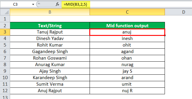
Example #1
In this MID formula example, we are fetching the substring from the given text string using the MID formula in excel =MID(B3,2,5). It will bring the substring from 2 characters and 5 letters from the 2nd position, and the output will be as shown in the second column.
Example #2
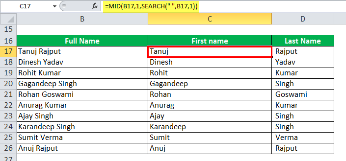
We can use the mid function that extracts the first and last names from the full names.
For First Name: here we have used the MID formula in Excel =MID(B17,1,SEARCH(” “,B17,1)); in this MID Formula example, the MID function searches the string at B17 and starts the substring from the first character, here search function fetches the location of space and return the integer value. In the end, both functions filter out the first name.
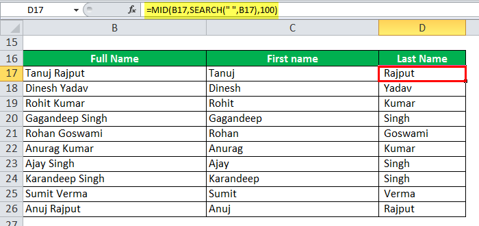
For the Last Name: Similarly, for the last name, use the =MID(B17,SEARCH(” “,B17),100), and it will give you the last name from the full name.
Example #3
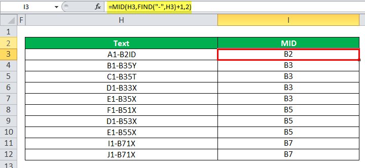
Suppose we have to find out the block from ID, which is located after “-“in ID, then use =MID(H3,FIND(“-“,H3)+1,2) MID formula in Excel to filter out the block ID two-character after.
Example #4
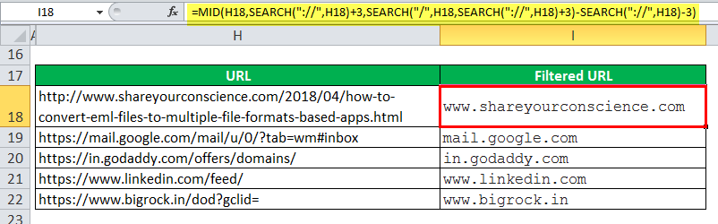
We can also find out the domain name from the web URLs. Here is the MID function used to achieve this:
=MID(H18,SEARCH(“://”,H18)+3,SEARCH(“/”,H18,SEARCH(“://”,H18)+3)-SEARCH(“://”,H18)-3)
Excel MID Function can be used as a VBA function.
Dim Midstring As String
Midstring = Application.worksheetfunction.mid(“Alphabet”, 5, 2)
Msgbox(Midstring) // Return the substring “ab” from string “Alphabet” in the message box.
The output will be “ab.”
Things to Remember About Excel MID Function
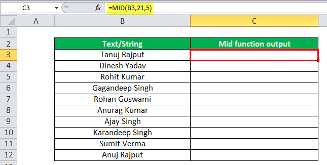
- Excel MID formula returns empty text if the start_num is greater than the length of the string.
=MID(B3,21,5)= blank as the start number is greater than the string length, so the output will be empty, as shown below.
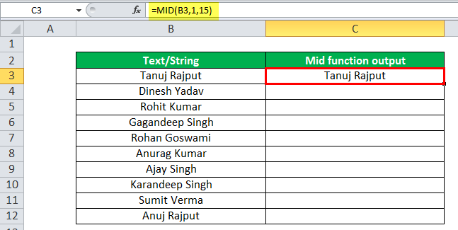
- If start_num is < the length of text, but start_num + num_chars exceeds the length of the string, then MID returns the characters up to the end of the text.
=MID(B3,1,15)
- The MID function in Excel through the #VALUE#VALUE! Error in Excel represents that the reference cell the user has either entered an incorrect formula or used a wrong data type (mostly numerical data). Sometimes, it is difficult to identify the kind of mistake behind this error.read more! Error
- If start_num < 1 ex. =MID(B3,-1,15)
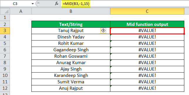
- If num_chars is a negative value.
=MID(B3,1,-15)

MID Excel Function Video
Recommended Articles
This article is a guide to MID Function in Excel. We discuss the MID formula in Excel and how to use the MID Excel formula along with the MID formula example and downloadable Excel templates. You may also look at these useful functions in Excel: –
- VBA MIDVBA MID function extracts the middle values from the supplied sentence or word. It is categorized under the String and Text function and is a worksheet function.read more
- INDEX FunctionThe INDEX function in Excel helps extract the value of a cell, which is within a specified array (range) and, at the intersection of the stated row and column numbers.read more
- RAND Excel FunctionThe RAND function in Excel, also known as the random function, generates a random value greater than 0 but less than 1, with an even distribution among those numbers when used on multiple cells. read more
- POWER in ExcelPOWER function calculates the power of a given number or base. To use this function you can use the keyword =POWER( in a cell and provide two arguments one as number and another as power.read more
- Frequency Distribution in ExcelFrequency distribution in excel is a calculation of the rate of a change happening over time in the data. By categorizing data in sets and applying the array formula frequency function or in the data analysis tab, use the histogram tool to determine frequency distribution.read more
Функция MID в Excel является функцией группы функций Text, вы используете функцию MID, если хотите вырезать строку в середине текстовой строки при обработке строки. Если вы не знаете или не понимаете функцию MID, вы можете обратиться к статье о том, как использовать функцию MID, с примером, показанным ниже.

В этой статье вы найдете описание, синтаксис и примеры использования функции MID. Приглашаем вас продолжить.
Функция MID — это функция, которая разрезает строку посередине, возвращая определенное количество символов из текстовой строки, а позиция для вырезания строки будет указана вами.
Функция MID всегда считает каждый символ как 1, будь то однобайтный или двухбайтный, независимо от языковых настроек по умолчанию?
Синтаксис функции MID
= MID (текст; начальное_число; число_символов)
Внутри:
- Текст — обязательный аргумент, это текстовая строка, содержащая символы, которые вы хотите получить.
- start_num — обязательный аргумент, это позиция первого символа, который функция MID должна принимать в текстовой строке.
- num_chars — обязательный аргумент, это количество символов, которое функция MID должна возвращать, начиная с позиции start_num.
Примечание
- Если num_chars (num_chars — отрицательное число), функция MID возвращает #VALUE! Значение ошибки.
- Если start_num, функция MID возвращает @VALUE! Значение ошибки.
- Если start_num больше длины текста, функция MID возвращает пустой текст (»).
- Если start_num меньше длины текста, но start_num плюс num_chars больше длины текстовой строки, функция MID возвращается от start_num к последнему символу текста.
Пример функции MID
Пример 1. Используйте функцию MID, чтобы извлечь 3 символа из строки «Функция MID в Excel», начиная с позиции 5.
Вы можете ввести строку непосредственно в функцию MID, где start_num равно 5, а количество символов, сокращающих num_chars, равно 3.
= MID («Функция MID в Excel»; 5; 3)
Или вы можете обратиться к ячейке, содержащей строку для извлечения.
Пример 2: Объедините функцию MID с функциями VLOOKUP, LEFT и IF для обработки следующей таблицы данных.
Как работать с ценой за единицу:
- Используя VLOOKUP для поиска 2 символов слева от кода заказа (используя LEFT) для поиска в таблице розничных / оптовых цен, возвращаемое значение функции VLOOKUP вы используете функцию IF, если 4-й символ в коде If заказ S, то будет возвращено соответствующее значение в графе 3 Прейскуранта. Если возвращается L (кроме S), будет возвращено соответствующее значение в четвертом столбце таблицы цен. Что касается функции ЕСЛИ, вам нужно разделить четвертый символ кода заказа — S или L.
Если вы не понимаете функцию VLOOKUP, вы можете узнать больше об использовании функции VLOOKUP здесь http://TipsMake.vn/ham-vlookup-in-excel/
В частности, вы вводите следующую формулу функции в ячейку E6
= ВПР (ЛЕВО (B6; 2); A16: D19; ЕСЛИ (MID (B6; 4; 1) = «S»; 3; 4); 0)
Внутри:
- LEFT (B6; 2) возвращает первые 2 символа в коде заказа, эти 2 символа являются строками для поиска.
- A16: D19 — это таблица обнаружения, которая представляет собой оптовый / розничный прайс-лист.
- IF (MID (B6; 4; 1) = «S»; 3; 4) Эта функция IF вернет значение 3 или 4, которое является позицией столбца, который возвращает соответствующие данные в таблице поиска.
- 0 — правильный тип обнаружения.
Затем, если вы хотите скопировать формулу функции Vlookup с помощью LEFT, IF, MID, тогда, когда вы вводите формулу Vlookup в оптовый / розничный прайс-лист A16: A19, нажмите клавишу F4, чтобы исправить это табличное пространство. Теперь функция Vlookup будет выглядеть так:
= ВПР (ЛЕВО (B6; 2); $ A $ 16: $ D $ 19; ЕСЛИ (MID (B6; 4; 1) = «S»; 3; 4); 0)
Вам просто нужно скопировать формулу.
Чтобы вычислить столбец Тхань Тьен, вам нужно всего лишь использовать оператор *, чтобы умножить SL Sales SL на найденную цену единицы и скопировать формулу в ячейки ниже. Итак, ваш лист данных обработан.
Таким образом, в статье используется общий синтаксис, например, как использовать функцию MID в Excel. Надеюсь, благодаря этой статье вы лучше поймете функцию MID. Вы можете гибко комбинировать функцию MID с другими функциями, чтобы получить от нее максимальную отдачу. Удачи!
Purpose
Extract text from inside a string
Return value
The characters extracted.
Usage notes
The MID function extracts a given number of characters from the middle of a supplied text string. MID takes three arguments, all of which are required. The first argument, text, is the text string to start with. The second argument, start_num, is the position of the first character to extract. The third argument, num_chars, is the number of characters to extract. If num_chars is greater than the number of characters available, MID returns all remaining characters.
Examples
The formula below returns 3 characters starting at the 5th character:
=MID("The cat in the hat",5,3) // returns "cat"
This formula will extract 3 characters starting at character 16:
=MID("The cat in the hat",16,3) // returns "hat"
If num_chars is greater than remaining characters, MID will all remaining characters:
=MID("apple",3,100) // returns "ple"
MID can extract text from numbers, but the result is text:
=MID(12348,3,4) // returns "348" as text
Related functions
Use the MID function to extract from the middle of text. Use the LEFT function to extract text from the left side of a text string and the RIGHT function to extract text starting from the right side of text. The LEN function returns the length of text as a count of characters. Use FIND or SEARCH to locate an unknown start position.
Notes
- num_chars is optional and defaults to 1.
- MID will extract text from numeric values, but the result is text
- Number formatting is not counted or extracted.
This post will guide you how to use Excel IF function with syntax and examples in Microsoft excel.
- Excel IF function Description
- Excel IF function Syntax
- Nested IF statements
- Excel Logical operators
- Frequently Asked Questions
- Related Functions
- Excel IF Formula Examples
Table of Contents
- Description
- Syntax
- Nested IF statements
- Excel Logical operators
- Frequently Asked Questions
- Related Functions
- More Excel IF Formula Examples
Description
The Excel IF function perform a logical test to return one value if the condition is TRUE and return another value if the condition is FALSE.
The IF function is a build-in function in Microsoft Excel and it is categorized as a Logical Function.
The IF function is available in Excel 2016, Excel 2013, Excel 2010, Excel 2007, Excel 2003, Excel XP, Excel 2000, Excel 2011 for Mac.
Syntax
The syntax of the IF function is as below:
= IF (condition, [true_value], [false_value])
Where the IF function arguments are:
Condition -This is a required argument. A user-defined condition that is to be tested.
True_value – This is an optional argument. The value that is returned if condition evaluates to TRUE.
False_value – This is an optional argument. The value that is returned if condition evaluates to FALSE.
The below examples will show you how to use Excel IF Function to return one value if the condition is TRUE or FALSE.
=IF(B1>90, good, bad)
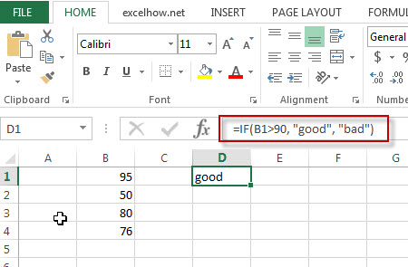
Note: the above excel formula will test a condition “b1>90”, if the condition is true, then “good” will return or “bad” will return.
Nested IF statements
The excel if function just only test one condition and if you want to deal with more than one condition and return different actions depending on the result of the tests, then you need to include several IF statements (functions) in one excel IF formula, these multiple IF statements are also called Excel Nested IF formula(Nested IFs).
For example:
=IF(A1>=80, "excellent", IF(A1>=60, "good", IF(A1>0, "bad", "no valid score")))
More reading: Excel Nexted IF Functions (Statements) Tutorial
Excel Logical operators
When you are writing an If statement, you may need to use any of the following excel logical operators:
| Operator | Meaning | Example | Description |
| = | Equal To | A1=B1 | Returns True if a value in cell A1 is equal to the values in cell B1; FALSE if they are not. |
| > | Greater Than | A1>B1 | Returns True if a value in cell A1 is greater than the values in cell B1; FALSE if they are not. |
| >= | Greater Than or Equal to | A1>=B1 | Returns True if a value in cell A1 is greater than or equal to the values in cell B1; FALSE if they are not. |
| < | Less Than | A1<B1 | Returns True if a value in cell A1 is less than the values in cell B1; FALSE if they are not. |
| <= | Less Than or Equal to | A1<=B1 | Returns True if a value in cell A1 is less than or equal to the values in cell B1; FALSE if they are not. |
| <> | Not Equal to | A1<>B1 | Returns True if a value in cell A1 is not equal to the values in cell B1; FALSE if they are not. |
Let’s see some examples for logical operators in Excel formula:
 =(A1>B1)
Output: TRUE

=(A1<B1)
Output: FALSE

=(A1>=B1)
Output: TRUE

=(A1<>8)
Output: FALSE

=(A1<>B1)
Output: TRUE

=(IF A1>3, “TRUE”, “FALSE”)
Output: TRUE
Frequently Asked Questions
Question1: I want to write an IF Formula based on the below test criteria in the Microsoft excel.
If the number in Cell B1 is greater than 30, then I want it to return A
If the number in cell B1 is between 20 and 30, then I want it to return B
If the number in Cell B1 is below 20, then I want it to return C
The below formula is what I currently write:
=IF(B1>30,"A",IF(B1<30,B1>20,"B","C"))
When I entered the above formula in the Cell C1, and it will return an Error.
Answer: You can use IF function in combination with AND function to reflect the above logic. So you can do it using the following formula:
=IF(B1>30,"A",IF(AND(B1>=20,B1<=30),"B","C"))
Or you can use another IF formula without AND function as follows:
=IF(B1>30,"A",IF(B1<20,"C","B"))
Question 2: I want to write a excel Formula for sales rep, If the sales are less than 10K, then the member will get no commission. If the sales are between 10 and 50K, then the member will get a 3% commission. If the sales are more than 50k, then the member will get 5% commission. Could you help me?
Answer: Based on the above description, we can use the following excel IF formula:
=IF(B1<10,0,IF(B1<50,B1*3%,B1*5%))
Question 3: I want to select students for the scholarship in school, and based on the student’s scores and attendance value, if the student scores more than 85 and has the attendance of more than 85%, then he/she will get the scholarship. Please help me how to write this formula based on my test criteria.
Answer: you can use the IF function with the AND function to check whether both of two conditions are met or not. If the test are met, then return “Yes”, otherwise returns “No”.
So you can use the following IF formula in Excel:
=IF(AND(B1>85, C1>85%),"Yes","No")
Question 4: I am trying to write an excel formula based on the following logic:
I want to enter a formula in Cell C1 that will Add B1, B2 and B3 or multiply B1 by 1, multiply B2 by 2, multiply B2 by 3, which action will be taken based on what you put in Cell D1.
Appreciated for any help. Thanks
Answer: Based on the above logic description, you need to use SUM function to count the sum of B1, B2 and B3. We can use the following IF formula:
=IF(D1="Add”,SUM(B1,B2,B3),IF(D1="Multiply",B1*B2*B3,"ERROR"))
Question 5: I am trying to write a formula in excel to check the employee number field and returns the relevant band of employee. I already have one IF formula, but I always return the first value of “A”. Could you help?
=IF(B1>=10,"A",IF(B1>=20,"B",IF(B1>=50,"C")))
Answer: when you write an IF nested formula, you need to start with the largest number first or start the smallest number first with less than or equal to operator.
1# start with the largest number first, we can write down the below formula:
=IF(B1>=50,"C",IF(B1>=20,"B",IF(B1>=10,"A")))
2# start with the smallest number first, you need to change the >= to <= , just see the below formula:
=IF(B1<=10,"A",IF(B1<=20,"B",IF(B1<=50,"C")))
Question 6: I want to write a Formula in excel to return “bad” if the cell B1 is either <100 or >500, otherwise, it should be returned the value of cell B1.
Answer: For the above logic test, we should use the OR function in the IF condition, so we can write down the below IF formula:
=IF(OR(B1>500,B1<100),"good",B1)
Question 7: I want to write a formula in excel using IF function to check if the cell B1 >10 and B1<20. If TRUE, returns “good”, If FALSE, returns “bad”
Answer: You can use IF function in combination with AND function to check the value of Cell B1, if cell B1 is greater than 10 and cell B1 is less than 20, then returns “good”, otherwise, it will return “bad”.
=IF(AND(B1>10,B1<20),"good","bad")
Question 8: I need to write a nested IF statement in excel 2013 to check the following logic:
If Cell B1 is less than 5, then multiply it by 5.
If Cell B1 is greater than or equal to 5 but less than 10, then multiply it by 10.
If cell B1 is greater than 10, then multiply it by 15.
Answer: This is a generic nested IF formula in excel, we can write the below nested IF statement to reflect the logic.
=IF(B1<5, B1*5, IF(B1<10, B1*10, B1*15))
Question 9: I want to write a formula to match the following logic in MS Excel 2013:
If A1*B1 <=10, then returns A
If A1*B1 >10 but A1*B1 <=20, then returns B
If A1*B1 >20 but A1*B1 <=30, then returns C
If A1*B1>30, then returns D
Answer: You can use IF function to build a Nested IF statement in combination with AND function to achieve it. Let’s write down the following IF formula:
=IF(A1*B1<=10,"A", IF(AND(A1*B1>10,A1*B1<=20),"B", IF(AND(A1*B1>20,a1*B1<=30,"C","D"))))
Question 10: I want to write an IF function to check if the value in cell B1 is blank or Text string or Numeric value, if the cell B1 is empty, then return “blank”, if the cell B1 is a text string, then return “Text”, if the value in cell B1 is a numeric value, then return “number”. Any help for this formula, thanks.
Answer: Based on the description, you need to use ISBLANK function to check if the value in cell b1 is blank or not. And need to use ISTEXT function to check if the value in cell B1 is a text string or not and need to use ISNUMBER function to check if the value in cell B1 is a number or not. So you can write a nested IF statements in combination with ISBLANK, ISTEXT and ISNUMBER functions in Excel as follows:
=IF(ISBLANK(B1),"blank", IF(ISTEXT(B1),"Text", IF(ISNUMBER(B1),"number")))
Question 11: I want to write a formula in excel to calculate the bonus for employees in company, if the employee salary is greater than or equal to $2000, then the bonus will be 10% of the salary , otherwise, the bonus will be 5% of the employee salary.
Answer: we need to check if the salary in Cell B1 (it’s the salary of the first employee) is greater than or equal to 2000. It the condition test is TRUE, then returns B1*10%, otherwise returns b1*5%. So we can write down the following IF formula in excel:
=IF(B1>=2000, B1*10%, B1*5%)
Question 12: In Microsoft Excel 2013, I want to create an IF function to check if any employee who have at least 10 years of experience and whose salary is greater than $5000, If TRUE, then the bonus will be 20% of salary.
Answer: you can use IF function in combination with AND function to check if the value in cell B1 is greater than or equal to 10 and the value in Cell C1 is greater than 5000. If both of two conditions are TRUE, then returns C1*20%, otherwise returns “No Bonus”.
Let’s write down the following IF statement as follows:
=IF(AND(B1>=10,C1>5000),C1*20%, "No Bonus")
Question 13: I want to create an IF formula in Excel 2013 to check the following text logic:
If B1<10, then multiply B1 by 1%, but the returned value is not less than 50.
If B1>10, then multiply B1 by 2%, but the returned value is not greater than 100.
Answer: To reflect the first test condition, you need to use MAX function to match the condition. To reflect the second test condition, you need to use MIN function to match that the returned value should not be greater than 100. So we can use the following excel IF formula:
=IF(B1<10, MAX(50,B1*1%), IF(B1>10, MIN(100,B1*5%)))
Question 14: I want to use IF function to check if B1 is greater than 10 and B2 is greater than 20 and B3 is less than 30, if TRUE, then returns “good”, otherwise, it should be returned “bad”. So How to create the IF formula based on the above test criteria to check three conditions at the same time.
Answer: you need to use AND function within the IF function in excel to create an IF formula as follows:
=IF(AND(B1>10,B2>20,B3<30),"good","bad")
Question 15: I have an IF formula that might cause a division by zero error, I don’t know how to avoid this kind of errors in Excel formula.
Answer: You can use ISERROR function to catch this kind of errors then use the IF function to check the returned values from ISERROR function to avoid an error. So we can write an IF function in combination with ISERROR function in excel. For example, we can use the following IF formula:
=IF(ISERROR(B1/C1),0, B1/C1)
The ISERROR function will return TRUE when trying to divide B1 by 0.
Question 16: I need to create a formula in Excel 2013 to reflect the following logic:
If B1=Excel, then return E
If B1=word, then return W
If B1=access, then return A
Answer: You can use IF function to create a nested IF statements as follows:
=IF(B1="Excel","E",IF(B1="word","W",IF(B1="access","A")))
Question 17: I have a worksheet that containing cells that are formatted as date format. I want to write an IF formula to check the first value in Cell (month part). So I am trying to create the following IF formula:
=IF(LEFT(B1,1)=8, "August","Null")
The returned results are always “Null”.
Answer: As the dates are not recognized as string, so you cannot use the LEFT function to exact the first value in the dates. At this moment, you need to use Month function to convert the date to its month number in Excel. So we can write down the below IF formula in combination with Month function:
=IF(MONTH(B1)=8, "August","Null")
Question18: I am trying to create an IF formula to check if the time value in cells are greater than 10.00h for the following date format: 08/11/2018 09:43.50. Appreciative of any help.
Answer: In excel, you can use HOUR, MINUTE, SECOND functions to compare the date or time value. so if you want to compare the value in Cell B1 if it is greater than 10h, then you can use HOUR function within IF function, just like this: HOUR(B1)>10, so we can write down the below formula:
=IF(HOUR(B1)>10, "greater","less")
Question 19: I want to create an IF function and need to combine with another RAND function. The formula just works find for the first IF_VALUE_TRUE statement, but the formula works not good for IF_VALUE_FALSE statement. Here is the IF formula I have got:
=IF(ISBLANK(B1),"","=rand()")
In the above IF function, it will return empty string when the value in cell B1 is blank. Otherwise, it should add a random function, the problem is that the cell doesn’t run the RAND function. So how can I fix it? Thanks
Answer: when you write an IF formula, if you want to enclose others function, you need not to add quotes around the RAND () function, so just remove the quotes and equal sign in your IF function. Just like the below IF formula:
=IF(ISBLANK(B1),"",RAND())
Question 20: I am trying to write an IF formula in Excel 2013 to reflect the following logic:
If B1 is greater than or equal to 50 and C1 is 0
OR
If B1 is greater than or equal to 30 and C1 is greater than or equal to 1
OR
If B1 is greater than or equal to 20 and C1 is 2
Then take the following action: D2/E2
Otherwise, return FALSE
I have wrote the following IF formula, but it doesn’t work at all.
=IF(AND(B1>=50,C1>=0),OR(AND(B1>=30,C1>=1)),OR(AND(B1>=20,C1>=2)),D2/E2,"FALSE")
Answer: you need to nest your different AND function within an OR function in the IF formula. So you can try the below IF formula:
=IF(OR(AND(B1>=50,C1>=0),AND(B1>=30,C1>=1),AND(B1>=20,C1>=2)), D2/E2,"FALSE")
Question 21: I want to create an IF function in combination with MID function in excel 2013. it need to check if the value in one specified cell is TRUE, then return the first six characters from another cell. Otherwise return empty value.
Answer: you just need to add MID function within IF function in excel, and do not add any quotes around MID function. So you can use the following IF formula to achieve your request:
=IF(B1=TRUE, MID(C1,1,5), "")
Question 22: I have a excel worksheet as below:
A B
——
20 O
30 V
10 T
50 T
I want to create an IF formula to reflect the following logic:
IF cell A1 is less than or equal to 30 and Cell B1 is equal to “O” or “V”, if TRUE, then returns 300, otherwise returns 400.
IF Cell A1 is greater than 30 and Cell B1 is equal to “O” or “V”, then returns 500, otherwise returns 600.
I have wrote the below tow IF formulas for the above two conditions as follows:
=IF(AND(A1<=30,OR(B1="O",B1="V")),300,400)
=IF(AND(A1>30,OR(B1="O",B1="V")),500,600)
I am able to check the above two IF formula and the returned results is OK… But I am not able to combine the above two IF formula into a single IF formula. So anybody can help? Many thanks
Answer: Based on the above logic, you can use the below IF formula to combine with above two IF formulas:
=IF(A1<=30,IF(OR(B1="O",B1="V"),300,400),IF(OR(B1="O",B1="V"),500,600))
Question 23: I am trying to write an IF function to prevent zero and negative values in cells. What I would like is that if the value in cell B1 is less than or equal to 0, then it should be returned “Null” otherwise, it should return the calculation of Cells value, like as:B2*(C2-D2)*E2.
The below IF formula is what I have:
=IF(B1<=0,"Null","B2*(C2-D2)*E2")
When I run the formula above, it only returns my calculation string and do not take the actual calculation.
Answer: In excel, the double quotes make any values in between be recognized as Text string. So if you want to take calculation for your IF formula, just remove the double quotes. Let’s see the modified IF formula as follows:
=IF(B1<=0,"Null",B2*(C2-D2)*E2)
Question 24: I want to create an new IF function to check if the value in cells is Saturday or Sunday, If TRUE, returns “yes”, otherwise, returns “No”. And I am using the following IF formula, but I get an error, so what’s wrong for this formula?
=IF((OR($B1="Saturday","$B1="Sunday"),"yes","no"))
Answer: you need to use the WEEKDAY function within IF function to handle the dates if they are in date format, like as: 11/8/2018.
So you can use the below IF function to achieve your logic:
=IF(WEEKDAY($B$1,2)>5,"yes","no")
You can also use TEXT function within the IF function to achieve the same results, just like the below IF formula:
=IF(LEFT(TEXT($B$1,"ddd"))="S","yes","no")
Question 25: I want to write an IF function in excel to check if the first character in one Cell is equal to 5, then the returned value should be the five rightmost characters of that cell, otherwise, the returned value should be the four rightmost characters. I wrote one IF formula as follows, but it doesn’t work.
=IF(LEFT(B1,1)=5, RIGHT(B1,5),RIGHT(B1,4))
In the above IF function, it always return the rightmost four characters even though the first character in Cell B1 starts with “S”. Please help me to fix it.
Answer: you should know the returned value of the LEFT function firstly in excel. As the LEFT function will return a Text value, so you also need to provide a string for comparison, so adding quotes to enclose it. Just like the below IF function:
=IF(LEFT(B1,1)="5", RIGHT(B1,5),RIGHT(B1,4))
There is another way to achieve the same results, you can use NUMBERVALUE function to convert the result of LEFT function to a numeric value, like the below IF function:
=IF(NUMBERVALUE(LEFT(B1,1))=5,RIGHT(B1,5),RIGHT(B1,4))
Question 26: I have 2 columns contain date and time or just only contain time. And I want to check if the times of column A is greater than the times of column B. the key issue may be that column A has the date and time. I wrote the following IF formula to run it in Cell C1, but it returned the inaccurate results.
=IF(A1>B1,"yes","no")
Any help would be appreciated… Many thanks!
Answer: the date part of the value in column A is the integer, while the time is the decimal. You can use the following IF formula:
=IF(A1-INT(A1)>B2),"yes","no")
Question 27: The below are the results that I expected, and I want cell B1 to B4 can detect the string from A1 to A4 automatically and return the same string value plus the severity level when the test match. For example, If A1 is equal to “critical”, then it should be returned “critical severity 1” in the cell B1. Etc.
And I am using the following IF formula, but it does not work at all. Please help to fix it. Thanks
=IF(A1="Critical","Critical Severity 1",""),IF(A1="High","High Severity 2",""),IF(A1="Medium","Medium Severity 3",""),IF(A1="Low","Low Severity 4","")
| A | B |
| critical | critical severity 1 |
| high | high severity 2 |
| medium | Medium severity 3 |
| low | low severity 4 |
Answer: you can try to run the following IF formula in excel:
=IF(A1="critical","critical Severity 1",IF(A1="high","high Severity 2",IF(A1="medium","medium Severity 3",IF(A1="low","low Severity 4",""))))
Question 28: I am working on an excel file and want to create a new IF formula to reflect the following logic:
If the value in Cell A1 is equal to the value in Cell A2, then check if the minus of B1 and B2 is equal to a special value, and if the condition is TRUE, returns “yes”, otherwise, returns “no”. Here is the IF formula I have:
=if(A1=A2,B1-B2=5 or B1-B2=-5 or B1-B2=20 or B1-B2=-20, "yes", "no")
Any help is appreciated…Thanks
Answer: you need to use OR function with IF function to create a nested IF statement to achieve your request. So you can try the following Excel IF formula in your excel file.
=IF(A1=A2,IF(OR(B1-B2=5,B1-B2=-5,B1-B2=20,B1-B2=-20),"yes","no"),"no")
Question 29: I want to create an IF formula to check the range of cells in excel. I have scores of different subject for a student, and want to check if any one of scores is less than 60, If TRUE, then return “BAD”. Can this logic be done with the IF statements in excel 2013?
Answer: you can use COUNTIF function within IF function to create a generic IF formula as follows:
=IF(COUNTIF(B:B,"<60")>0,"BAD","Good")
Question 30: I am trying to create a new IF statement so that when the formula is looking at Row A and Row B, the returned values should be shown in the Row C. the following logic need to be checked:
IF the value in the Row A is equal to “NA” And the value in the Row B is equal to “NA”, then return “NA” value in Row C.
IF the value in the Row A is equal to “NA”, and the value in the Row B is equal to “denied”, then return “denied” value in Row C.
IF the value in the Row A is equal to “allowed” and the value in the Row B is equal to “NA”, then return “allowed” value in Row C.
Here is my formula:
=IF(AND(A1 = "NA", B1 = "NA"),"NA",IF(OR(A1="denied",B1 ="denied"),"denied", "NA"))
I don’t know how to include “allowed” in the IF formula above, anyone can help this, many thanks.
Answer: This is a typical nested if statement, you can use OR function within IF function in excel. We can write down this nested IF formula as follows:
=IF(OR(A1="denied", B1="denied"), "denied", IF(OR(A1="allowed", B1="allowed"), "allowed", "NA"))
- Excel AND function
The Excel AND function returns TRUE if all of arguments are TRUE, and it returns FALSE if any of arguments are FALSE.The syntax of the AND function is as below:= AND (condition1,[condition2],…) … - Excel ISBLANK function
The Excel ISBLANK function returns TRUE if the value is blank or null.The syntax of the ISBLANK function is as below:= ISBLANK (value)… - Excel COUNTIF function
The Excel COUNTIF function will count the number of cells in a range that meet a given criteria.= COUNTIF (range, criteria) … - Excel ISERROR function
The Excel ISERROR function returns TRUE if the value is any error value except #N/A. The ISERROR function is a build-in function in Microsoft Excel and it is categorized as an Information Function. The syntax of the ISERROR function is as below: = ISERROR (value) … - Excel LEFT function
The Excel LEFT function returns a substring (a specified number of the characters) from a text string, starting from the leftmost character.The syntax of the LEFT function is as below:= LEFT(text,[num_chars])… - Excel MID function
The Excel MID function returns a substring from a text string at the position that you specify. The MID function is a build-in function in Microsoft Excel and it is categorized as a Text Function. The syntax of the MID function is as below: = MID (text, start_num, num_chars) … - Excel TEXT function
The Excel TEXT function converts a numeric value into text string with a specified format. The syntax of the TEXT function is as below:= TEXT (value, Format code)… - Excel RIGHT function
The Excel RIGHT function returns a substring (a specified number of the characters) from a text string, starting from the rightmost character…
More Excel IF Formula Examples
- Excel nested if function
The nested IF function is formed by multiple if statements within one Excel if function. This excel nested if statement makes it possible for a single formula to take multiple actions… - Excel IF formula with Equal to logical operators
The “Equal to” logical operator can be used to compare the below data types, such as: text string, numbers, dates, Booleans. This section will guide you how to use equal to logical operator in excel IF formula with text string value and dates value… - Excel IF formula with greater than logical operators
How to use if function with greater than, greater than or equal to, less than and less than or equal to logical operators in excel. Let’s see the below generic if formula with greater than operator: =IF(A1>10,”excelhow.net”,”google”) … - Excel IF formula with AND logical function
You can use the IF function combining with AND function to construct a condition statement. If the test is FALSE, then take another action. The syntax of AND function in excel is as follow: =AND(condition1,[condition2],…)… - Excel IF function with OR logical function
If you want to check if one of several conditions is met in your excel workbook, if the test is TRUE, then you can take certain action. You can use the IF function combining with OR function to construct a condition statement… - Excel IF function with “NOT” logical function
If you want to check several test conditions in an excel formula, then take different actions. You can use NOT function in combination with the AND or OR logical function in excel IF function… - Excel IF formula with AND & OR logical functions
If you want to test the result of cells based on several sets of multiple test conditions, you can use the IF function with the AND and OR functions at a time… - Excel IF Function With Numbers
If you want to check if a cell values is between two values or checking for the range of numbers or multiple values in cells, at this time, we need to use AND or OR logical function in combination with the logical operator and IF function… - Excel IF function with text values
If you want to write an IF formula for text values in combining with the below two logical operators in excel, such as: “equal to” or “not equal to”… - Excel IF function with Dates
If you have a list of dates and then want to compare to these dates with a specified date to check if those dates is greater than or less than that specified date. … - Excel IF function check if the cell is blank or not-blank
If you want to check the value in one cell if it is blank or empty cell, then you can use IF function in combination with ISBLANK function or logical operator (equal to) in excel… -
Excel nested if statements with ranges
Many people usually asked that how to write an excel nested if statements based on multiple ranges of cells to return different values in a cell? How to nested if statement using date ranges? How to use nested if statement between different values in excel 2013 or 2016… - Count Cells That Contain Specific Text
This post will discuss that how to count the number of cells that contain specific text or certain text in a specified cells of range in Excel. How to get the total number of cells that contain certain text.…… - Sum Values by Group
Assuming that you have a table that contain the product name and its sales result. And you have group by those values based on the product name, then you want to sum values based one each product name. You can create a new Excel formula based on the IF function and SUMIF function.… - Get nth Largest Value with Duplicates
If you want to get the largest unique value in a data set with duplicates, you can create a new excel array formula based on the MAX function and the IF function..… - Find the Largest Value Based on Multiple Criteria
Assuming that you have a list of data that you want to find the largest value based on the product “excel” and the sales region “east”. You can create a new excel formula based on the SUMPRODUCT function and the LARGE function..…… - Create a Five Star Rating System
How do I change the five points system to five star rating in excel. How to use the conditional formatting function to create a five star rating system in excel….. - Rank values in a column based a specific value in another column
Assuming that you have a list of data contains two columns and the first column is product list and another is Sales number. You want to rank the sales number of a specified product name. You can try to write a complex formula based on the IF function and the COUNTIFS function to achieve the result..… - Comparing Columns Using Conditional Formatting Icon Sets
how to compare the adjacent cells in the different columns using Conditional Formatting Icon Sets in Excel. How to compare Columns or rows using Conditional Formatting Icon Sets to show increase or decrease status in your current worksheet..… - Show Only Positive Values
You can create a formula based on the IF function, and the SUM function to sum all values in the range A1:C5 and just show only positive values… - Count Unique Values Using Pivot Table
You can insert a 3rd or helper column with a formula to check if the value is unique in the selected range of cells, and the create pivot table based on the 1st and 3rd column to count unique values..… - Compare Dates
Assuming that you have a list of data that contain date values in Excel, you can use the IF function to create a formula to achieve it. If the date is greater that the given date value, then return True. Otherwise, it returns False…. - Excel Vlookup Return True or False
you can use the VLOOKUP function to look for a value in a column in a table and then returns TRUE from a given column in that table if it finds something. If it doesn’t, it returns FALSE … - VLOOKUP Return Multiple Values Horizontally
You can create a complex array formula based on the INDEX function, the SMALL function, the IF function, the ROW function and the COLUMN function to vlookup a value and then return multiple corresponding values horizontally in Excel.… - Copy and Paste Only Non-blank Cells
If you want only copy non-blank cells in a range in Excel, you need to select the non-blank cells firstly, then press Ctrl +C keys to copy the selected cells. So how to only select all non-blank cells in the selected range in your worksheet..… - Changing Negative Number to Zero in Excel
If you want to change all negative numbers to zero value from a cell in Excel, you can use a formula based on the MAX function or IF function.… - Count Dates in Given Year/Month/Day in Excel
You can create a formula based on the SUMPRODUCT function and the YEAR function to count dates by a give year…. - Generate All Possible Combinations of Two Lists
You can use a formula based on the IF function, the ROW function, the COUNTA function, The INDEX function and the MOD function to get a list of all possible combinations from those two list…. - Find Missing Numbers in a Sequence in Excel
You can use an excel array formula based on the SMALL function, the IF function, the ISNA function, the MATCH function, and the ROW function to find missing numbers in a sequence…