If function excel name - Word и Excel - помощь в работе с программами

IF function

The IF function is one of the most popular functions in Excel, and it allows you to make logical comparisons between a value and what you expect.

So an IF statement can have two results. The first result is if your comparison is True, the second if your comparison is False.

For example, =IF(C2=”Yes”,1,2) says IF(C2 = Yes, then return a 1, otherwise return a 2).

Use the IF function, one of the logical functions, to return one value if a condition is true and another value if it’s false.

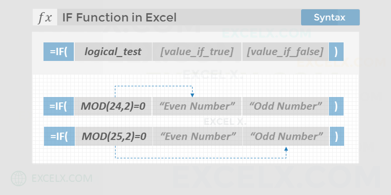
IF(logical_test, value_if_true, [value_if_false])

For example:

=IF(A2>B2,»Over Budget»,»OK»)
=IF(A2=B2,B4-A4,»»)

Argument name	Description
logical_test (required)	The condition you want to test.
value_if_true (required)	The value that you want returned if the result of *logical_test* is TRUE.
value_if_false (optional)	The value that you want returned if the result of *logical_test* is FALSE.

Simple IF examples

=IF(C2=”Yes”,1,2)

In the above example, cell D2 says: IF(C2 = Yes, then return a 1, otherwise return a 2)

=IF(C2=1,”Yes”,”No”)

In this example, the formula in cell D2 says: IF(C2 = 1, then return Yes, otherwise return No)As you see, the IF function can be used to evaluate both text and values. It can also be used to evaluate errors. You are not limited to only checking if one thing is equal to another and returning a single result, you can also use mathematical operators and perform additional calculations depending on your criteria. You can also nest multiple IF functions together in order to perform multiple comparisons.

=IF(C2>B2,”Over Budget”,”Within Budget”)

In the above example, the IF function in D2 is saying IF(C2 Is Greater Than B2, then return “Over Budget”, otherwise return “Within Budget”)

=IF(C2>B2,C2-B2,0)

In the above illustration, instead of returning a text result, we are going to return a mathematical calculation. So the formula in E2 is saying IF(Actual is Greater than Budgeted, then Subtract the Budgeted amount from the Actual amount, otherwise return nothing).

=IF(E7=”Yes”,F5*0.0825,0)

In this example, the formula in F7 is saying IF(E7 = “Yes”, then calculate the Total Amount in F5 * 8.25%, otherwise no Sales Tax is due so return 0)

Note: If you are going to use text in formulas, you need to wrap the text in quotes (e.g. “Text”). The only exception to that is using TRUE or FALSE, which Excel automatically understands.

Common problems

Problem	What went wrong
0 (zero) in cell	There was no argument for either value_if_true or value_if_False arguments. To see the right value returned, add argument text to the two arguments, or add TRUE or FALSE to the argument.
#NAME? in cell	This usually means that the formula is misspelled.

Need more help?

You can always ask an expert in the Excel Tech Community or get support in the Answers community.

What is IF Function in Excel?

IF function in Excel evaluates whether a given condition is met and returns a value depending on whether the result is “true” or “false”. It is a conditional function of Excel, which returns the result based on the fulfillment or non-fulfillment of the given criteria.

For example, the IF formula in Excel can be applied as follows:

“=IF(condition A,“value B”,“value C”)”

The IF excel function returns “value B” if condition A is met and returns “value C” if condition A is not met.

It is often used to make logical interpretations which help in decision-making.

What is IF Function in Excel?
- Syntax of the IF Excel Function
- How to Use IF Function in Excel?
  - Example #1
  - Example #2
  - Example #3
  - Example #4
  - Example #5
- Guidelines for the Multiple IF Statements
- Frequently Asked Question
- IF Excel Function Video
- Recommended Articles

Syntax of the IF Excel Function

The syntax of the IF function is shown in the following image:

The IF excel function accepts the following arguments:

Logical_test: It refers to the condition to be evaluated. The condition can be a value or a logical expression.
Value_if_true: It is the value returned as a result when the condition is “true”.
Value_if_false: It is the value returned as a result when the condition is “false”.

In the formula, the “logical_test” is a required argument, whereas the “value_if_true” and “value_if_false” are optional arguments.

The IF formula uses logical operators to evaluate the values in a range of cells. The following table shows the different logical operatorsLogical operators in excel are also known as the comparison operators and they are used to compare two or more values, the return output given by these operators are either true or false, we get true value when the conditions match the criteria and false as a result when the conditions do not match the criteria.read more and their meaning.

Operator	Meaning
=	Equal to
>	Greater than
>=	Greater than or equal to
<	Less than
<=	Less than or equal to
<>	Not equal to

How to Use IF Function in Excel?

Let us understand the working of the IF function with the help of the following examples in Excel.

You can download this IF Function Excel Template here – IF Function Excel Template

Example #1

If there is no oxygen on a planet, life is impossible. If oxygen is available on a planet, then life is possible. The following table shows a list of planets in column A and the information on the availability of oxygen in column B. We have to find the planets where life is possible, based on the condition of oxygen availability.

Let us apply the IF formula to cell C2 to find out whether life is possible on the planets listed in the table.

The IF formula is stated as follows:

“=IF(B2=“Yes”, “Life is Possible”, “Life is Not Possible”)

The succeeding image shows the IF formula applied to cell C2.

The subsequent image shows how the IF formula is applied to the range of cells C2:C5.

Drag the cells to view the output of all the planets.

The output in the below worksheet shows life is possible on the planet Earth.

Flow Chart of Generic IF Excel Function

The IF Function Flow Chart for Mars (Example #1)

The flow of IF function flowchart for Jupiter and Venus is the same as the IF function flowchart for Mars (Example #1).

The IF Function Flow Chart for Earth

Hence, the IF excel function allows making logical comparisons between values. The modus operandi of the IF function is stated as: If something is true, then do something; otherwise, do something else.

Example #2

The following table shows a list of years. We want to find out if the given year is a leap year or not.

A leap year has 366 days; the extra day is the 29th of February. The criteria for a leap year are stated as follows:

The year will be exactly divisible by 4 and not exactly be divisible by 100 or
The year will be exactly divisible by 400.

In this example, we will use the IF function along with the AND, OR, and MOD functions to find the leap years.

We use the MOD function to find a remainder after a dividend is divided by a divisor.

The AND functionThe AND function in Excel is classified as a logical function; it returns TRUE if the specified conditions are met, otherwise it returns FALSE.read more evaluates both the conditions of the leap years for the value “true”. The OR functionThe OR function in Excel is used to test various conditions, allowing you to compare two values or statements in Excel. If at least one of the arguments or conditions evaluates to TRUE, it will return TRUE. Similarly, if all of the arguments or conditions are FALSE, it will return FASLE.read more evaluates either of the condition for the value “true”.

We will apply the MOD function to the conditions as follows:

If MOD(year,4)=0 and MOD(year,100)<>(is not equal to) 0, then the year is a leap year.

If MOD(year,400)=0, then the year is a leap year; otherwise, the year is not a leap year.

The IF formula is stated as follows:

“=IF(OR(AND((MOD(year,4)=0),(MOD(year,100)<>0)),(MOD(year,400)=0)),“Leap Year”, “Not A Leap Year”)”

The argument “year” refers to a reference value.

The following images show the output of the IF formula applied in the range of cells.

The following image shows how the IF formula is applied to the range of cells B2:B18.

The succeeding table shows the years 1960, 2028, and 2148 as leap years and the remaining as non-leap years.

The result of the IF excel formula is displayed for the range of cells B2:B18 in the following image.

Example #3

The succeeding table shows a list of drivers and the directions they undertook to reach the destination. It is preceded by an image of the road intersection explaining the turns taken by the drivers and their destinations. The right turn leads to town B, and the left turn leads to town C. Identify the driver’s destination to town B and town C.

Road Intersection Image

Let us apply the IF excel function to find the destination. Here, the condition is mentioned as follows:

If the driver turns right, he/she reaches town B.
If the driver turns left, he/she reaches town C.

We use the following IF formula to find the destination:

“=IF(B2=“Left”, “Town C”, “Town B”)”

The succeeding image shows the output of the IF formula applied to cell C2.

Drag the cells to use the formula in the range C2:C11. Finally, we get the destinations of each driver for their turning movements.

The below image displays the IF formula applied to the range.

The output of the IF formula and the destinations are displayed in the succeeding image.

The result shows that six drivers reached town C, and the remaining four have reached town B.

Example #4

The following table shows a list of items and their inventory levels. We want to check if the specific item is available in the inventory or not using the IF function.

Let us list the name of items in column A and the number of items in column B. The list of data to be validated for the entire items list is shown in the cell E2 of the below image.

We use the Excel IF along with the VLOOKUP functionThe VLOOKUP excel function searches for a particular value and returns a corresponding match based on a unique identifier. A unique identifier is uniquely associated with all the records of the database. For instance, employee ID, student roll number, customer contact number, seller email address, etc., are unique identifiers.
read more to check the availability of the items in the inventory.

The VLOOKUP function looks up the values referring to the number of items, and the IF function will check whether the item number is greater than zero or not.

We will apply the following IF formula in the F2 cell:

“=IF(VLOOKUP(E2,A2:B11,2,0)=0, “Item Not Available”,“Item Available”)”

If the lookup value of an item is equal to 0, then the item is not available; else, the item is available.

The succeeding image shows the result of the IF formula in the cell F2.

Select “bat” in the E2 item cell to know whether the item is available or not in the inventory (as shown in the following image).

Example #5

The following table shows the list of students and their marks. The grade criteria are provided based on the marks obtained by the students. We want to find the grade of each student in the list.

We apply the Nested IF in Excel since we have multiple criteria to find and decide each student’s grade.

The Nesting of IF function uses the IF function inside another IF formula when multiple conditions are to be fulfilled.

The syntax of Nesting of IF function is stated as follows:

“=IF( condition1, value_if_true1, IF( condition2, value_if_true2, value_if_false2 ))”

The succeeding table represents the range of scores and the grades, respectively.

Let us apply the multiple IF conditions with AND function in the below-nested formula to find out the grade of the students:

“=IF((B2>=95),“A”,IF(AND(B2>=85,B2<=94),“B”,IF(AND(B2>=75,B2<=84),“C”,IF(AND(B2>=61,B2<=74),“D”,“F”))))”

The IF function checks the logical condition as shown in the formula below:

“=IF(logical_test, [value_if_true],[value_if_false])”

We will split the above-mentioned nested formula and check the IF statements as shown below:

First Logical Test: B2>=95

If the formula returns,

Value_if_true, execute: “A” (Grade A) else(comma) enter value_if_false
Value_if_false, then the formula finds another IF condition and enter IF condition

Second Logical Test: B2>=85(logical expression 1) and B2<=94(logical expression 2)

(We use AND function to check the multiple logical expressions as the two given conditions are to be evaluated for “true.”)

If the formula returns,

Value_if_true, execute: “B” (Grade B) else(comma) enter value_if_false
Value_if_false, then the formula finds another IF condition and enter IF condition

Third Logical Test: B2>=75(logical expression 1) and B2<=84(logical expression 2)

(We use AND function to check the multiple logical expressions as the two given conditions are to be evaluated for “true.”)

If the formula returns,

Value_if_true, execute: “C” (Grade C) else(comma) enter value_if_false
value_if_false, then the formula finds another IF condition and enter IF condition

Fourth Logical Test: B2>=61(logical expression 1) and B2<=74(logical expression 2)

(We use AND function to check the multiple logical expressions as the two given conditions are to be evaluated for “true.”)

If the formula returns,

Value_if_true, execute: “D” (Grade D) else(comma) enter value_if_false

Value_if_false, execute: “F” (Grade F)
Finally, close the parenthesis.

The below image displays the output of the IF formula applied to the range.

The succeeding image shows the IF nested formula applied to the range.

The grades of the students are listed in the following table.

Guidelines for the Multiple IF Statements

The guidelines for the multiple IF statements are listed as follows:

Use nested IF function to a limited extent as multiple IF statements require a great deal of thought to be accurate.
Multiple IF statementsIn Excel, multiple IF conditions are IF statements that are contained within another IF statement. They are used to test multiple conditions at the same time and return distinct values. Additional IF statements can be included in the ‘value if true’ and ‘value if false’ arguments of a standard IF formula.read more require multiple parentheses (), which is often difficult to manage. Excel provides a way to check the color of each opening and closing parenthesis to avoid this situation. The last closing parenthesis color will always be black, denoting the end of the formula statement.
Whenever we pass a string value for the arguments “value_if_true” and “value_if_false” or test a reference against a string value, enclose the string value in double quotes. Passing a string value without quotes will result in “#NAME?” error.

Frequently Asked Question

1. What is the IF function in Excel?

The Excel IF function is a logical function that checks the given criteria and returns one value for a “true” and another value for a “false” result.

The syntax of the IF function is stated as follows:
“=IF(logical_test, [value_if_true], [value_if_false])”

The arguments are as follows:
1. Logical_test – It refers to a value or condition that is tested.
2. Value_if_true – It is the value returned when the condition logical_test is “true.”
3. Value_if_false – It is the value returned when the condition logical_test is “false.”

The “logical_test” is a required argument, whereas the “value_if_true” and “value_if_false” are optional arguments.

2. How to use the IF Excel function with multiple conditions?

The IF Excel statement for multiple conditions is created by using multiple IF functions in a single formula.

The syntax of IF function with multiple conditions is stated as follows:

“=IF (condition 1_“true”, do something, IF (condition 2_“true”, do something, IF (condition 3_ “true”, do something, else do something)))”

3. How to use the function IFERROR in Excel?

IF Excel Function Video

Что возвращает функция

Заданное вами значение при выполнении двух условий ИСТИНА или ЛОЖЬ.

Синтаксис

=IF(logical_test, [value_if_true], [value_if_false]) — английская версия

=ЕСЛИ(лог_выражение; [значение_если_истина]; [значение_если_ложь]) — русская версия

Аргументы функции

logical_test (лог_выражение) — это условие, которое вы хотите протестировать. Этот аргумент функции должен быть логичным и определяемым как ЛОЖЬ или ИСТИНА. Аргументом может быть как статичное значение, так и результат функции, вычисления;
[value_if_true] ([значение_если_истина]) — (не обязательно) — это то значение, которое возвращает функция. Оно будет отображено в случае, если значение которое вы тестируете соответствует условию ИСТИНА;
[value_if_false] ([значение_если_ложь]) — (не обязательно) — это то значение, которое возвращает функция. Оно будет отображено в случае, если условие, которое вы тестируете соответствует условию ЛОЖЬ.

Дополнительная информация

В функции ЕСЛИ может быть протестировано 64 условий за один раз;
Если какой-либо из аргументов функции является массивом — оценивается каждый элемент массива;
Если вы не укажете условие аргумента FALSE (ЛОЖЬ) value_if_false (значение_если_ложь) в функции, т.е. после аргумента value_if_true (значение_если_истина) есть только запятая (точка с запятой), функция вернет значение “0”, если результат вычисления функции будет равен FALSE (ЛОЖЬ).
На примере ниже, формула =IF(A1> 20,”Разрешить”) или =ЕСЛИ(A1>20;»Разрешить») , где value_if_false (значение_если_ложь) не указано, однако аргумент value_if_true (значение_если_истина) по-прежнему следует через запятую. Функция вернет “0” всякий раз, когда проверяемое условие не будет соответствовать условиям TRUE (ИСТИНА).

|
Если вы не укажете условие аргумента TRUE(ИСТИНА) (value_if_true (значение_если_истина)) в функции, т.е. условие указано только для аргумента value_if_false (значение_если_ложь), то формула вернет значение “0”, если результат вычисления функции будет равен TRUE (ИСТИНА);
На примере ниже формула равна =IF (A1>20;«Отказать») или =ЕСЛИ(A1>20;»Отказать»), где аргумент value_if_true (значение_если_истина) не указан, формула будет возвращать “0” всякий раз, когда условие соответствует TRUE (ИСТИНА).

Функция Если в Excel примеры с несколькими условиями

Пример 1. Проверяем простое числовое условие с помощью функции IF (ЕСЛИ)

При использовании функции ЕСЛИ в Excel, вы можете использовать различные операторы для проверки состояния. Вот список операторов, которые вы можете использовать:

Ниже приведен простой пример использования функции при расчете оценок студентов. Если сумма баллов больше или равна «35», то формула возвращает “Сдал”, иначе возвращается “Не сдал”.

Пример 2. Использование вложенной функции IF (ЕСЛИ) для проверки условия выражения

Функция может принимать до 64 условий одновременно. Несмотря на то, что создавать длинные вложенные функции нецелесообразно, то в редких случаях вы можете создать формулу, которая множество условий последовательно.

В приведенном ниже примере мы проверяем два условия.

Первое условие проверяет, сумму баллов не меньше ли она чем 35 баллов. Если это ИСТИНА, то функция вернет “Не сдал”;
В случае, если первое условие — ЛОЖЬ, и сумма баллов больше 35, то функция проверяет второе условие. В случае если сумма баллов больше или равна 75. Если это правда, то функция возвращает значение “Отлично”, в других случаях функция возвращает “Сдал”.

Пример 3. Вычисляем сумму комиссии с продаж с помощью функции IF (ЕСЛИ) в Excel

Функция позволяет выполнять вычисления с числами. Хороший пример использования — расчет комиссии продаж для торгового представителя.

В приведенном ниже примере, торговый представитель по продажам:

не получает комиссионных, если объем продаж меньше 50 тыс;
получает комиссию в размере 2%, если продажи между 50-100 тыс
получает 4% комиссионных, если объем продаж превышает 100 тыс.

Рассчитать размер комиссионных для торгового агента можно по следующей формуле:

=IF(B2<50,0,IF(B2<100,B2*2%,B2*4%)) — английская версия

=ЕСЛИ(B2<50;0;ЕСЛИ(B2<100;B2*2%;B2*4%)) — русская версия

В формуле, использованной в примере выше, вычисление суммы комиссионных выполняется в самой функции ЕСЛИ. Если объем продаж находится между 50-100K, то формула возвращает B2 * 2%, что составляет 2% комиссии в зависимости от объема продажи.

Больше лайфхаков в нашем Telegram Подписаться

Пример 4. Используем логические операторы (AND/OR) (И/ИЛИ) в функции IF (ЕСЛИ) в Excel

Вы можете использовать логические операторы (AND/OR) (И/ИЛИ) внутри функции для одновременного тестирования нескольких условий.

Например, предположим, что вы должны выбрать студентов для стипендий, основываясь на оценках и посещаемости. В приведенном ниже примере учащийся имеет право на участие только в том случае, если он набрал более 80 баллов и имеет посещаемость более 80%.

Вы можете использовать функцию AND (И) вместе с функцией IF (ЕСЛИ), чтобы сначала проверить, выполняются ли оба эти условия или нет. Если условия соблюдены, функция возвращает “Имеет право”, в противном случае она возвращает “Не имеет право”.

Формула для этого расчета:

=IF(AND(B2>80,C2>80%),”Да”,”Нет”) — английская версия

=ЕСЛИ(И(B2>80;C2>80%);»Да»;»Нет») — русская версия

Пример 5. Преобразуем ошибки в значения “0” с помощью функции IF (ЕСЛИ)

С помощью этой функции вы также можете убирать ячейки содержащие ошибки. Вы можете преобразовать значения ошибок в пробелы или нули или любое другое значение.

Формула для преобразования ошибок в ячейках следующая:

=IF(ISERROR(A1),0,A1) — английская версия

=ЕСЛИ(ЕОШИБКА(A1);0;A1) — русская версия

Формула возвращает “0”, в случае если в ячейке есть ошибка, иначе она возвращает значение ячейки.

ПРИМЕЧАНИЕ. Если вы используете Excel 2007 или версии после него, вы также можете использовать функцию IFERROR для этого.

Точно так же вы можете обрабатывать пустые ячейки. В случае пустых ячеек используйте функцию ISBLANK, на примере ниже:

=IF(ISBLANK(A1),0,A1) — английская версия

=ЕСЛИ(ЕПУСТО(A1);0;A1) — русская версия

Источник

In this tutorial, we will learn about the IF function in Excel. Along with IF, the AND and OR functions are important formulas too. A nested IF simply means multiple IF functions in a single syntax.

Introducing IF Function in Excel

Let’s get started with this easy guide to using the IF function and all its related functions in Microsoft Excel, step-by-step with supporting images and examples.

1. IF Function

To learn to use the IF function, we will take an example of a mark list of students below.

Our goal is to find out which student has passed or failed and what are their grades. Of course, it would be a tedious task to find out pass or fail results and grades for each student in this list.

To ease our task, we have IF functions for that matter. The IF function will automatically identify if a student has passed or failed based on the criteria you provide to it.

It will automatically mark a student as “Pass” if he/she has scored above the minimum pass mark and mark a student as “Fail” if he/she has scored below the minimum pass mark.

The IF function automatically assigns the appropriate grades to students based on their marks if you command it.

Here is a glimpse of how the IF function helps you out with assigning grades and marking “Pass” or “Fail”.

Steps to use IF function in Excel

We have allotted certain grades and marked them as Pass or Fail to students based on the percentages they have secured in their exams, with the help of the IF function.

1. Using the IF function in Excel to identify passed/failed students

Let’s learn how we can use the IF formula to achieve this. We will use the same example. We take the minimum passing percentage as 34%.

Find out the percentage of total marks of every student.
Create a new column named “Pass/Fail”.
In the blank cell below the title, type the IF formula as follows next.
Type =IF( and select the first student’s percentage and type >=34.
Put a comma and move to the next argument named [value_if_true]. This means you’re being asked to put a value to be displayed if the above condition is true. Remember these arguments are case sensitive.
Once you have put a comma, type “Pass”.
Put a comma and move to the next argument named [value_if_false] to display a value when the above condition is false. This field is optional in most cases but we need a false value because it is a mark list.
Close the bracket and hit ENTER.

You can see that the formula is displaying “Pass” for the first student because she has secured above 34%.

Double-click or drag the cell from the right corner below to autofill the formula to all the students below.

Recommended read: How to Autofill in Excel?

2. Nested IF Function

Now, let us start assigning grades to all students.

We are going to be using multiple IF functions in a single syntax this time to provide multiple criteria to the IF function. This is called Nested IF in Excel.

However, there is no specific function named “Nested IF” in Excel, it is simply that this behavior has been given a name i.e., Nested IF.

Before we proceed further, we need to first make a table that displays a grading class for each grade. Here is an example below.

Create a new column named “Grade”.
Type the IF function in a blank cell below the title as follows.
Type =IF( and now type AE118>=85,”A”,IF(AE118>=70,”B”,IF(AE118>=55,”C”,IF(AE118>=34,”D”,IF(AE118<=33,”Fail”.

Note that AE118 is our cell address for the first student’s percentage. It will be different in your case. Refer to the image above to make sense of the formula.
The formula simply states- if percentage marks are above and equal to 85 then give “A”, if percentage marks are above and equal to 70 then give “B”, and so on and so forth. For the last condition, we have applied the condition- if the marks are less than or equal to 33 then give “Fail”.
For the last IF statement, you can either put the result as “Fail” or “E” as you like.
Now, note that we will close the formula with 5 brackets for this example as we have used a total of 5 IF formulas.

Hit ENTER to complete the formula.

You can now see that the formula has been applied to the first entry and the result is B because the student has secured 72.5% which is less than 75%. This means the nested Ifs are working correctly.

Now drag the cell from the lower right corner to autofill the formula to the rest of the entries.

You can see that we now have grades and pass/fail markings for every student on the list successfully.

3. IF with AND in Excel

Let us learn the IF formula with the AND function in a single syntax with a minor example.

When you have two or more distinct conditions to be used together, you can use the IF function with AND in Excel.

While nested IFs will also work, using AND function will save your time as it is shorter to type. So, let’s get started.

Our goal is to identify currencies with revenues greater than 20,000 and less than 50,000 and mark them as “Good”.

Type =IF(AND( because we are using the IF with AND function.
Select the first cell under Revenue, and type >20000.
Put a comma and select the first cell under Revenue again and type <50000.
Now, close the bracket to complete the AND function. We’re still working on the IF function so do not put two brackets.
We come back to the IF function as soon as we close the AND function. Now put the values to be displayed if the condition is true or false.
Put a comma to move to the argument [value_if_true] and type “Good”.
You can provide a result in the [value_if_false] argument, but it is completely optional. If nothing is provided then the cells will display FALSE if the condition is false. But if you want the cells to remain blank simply put “” (two double quotation marks) in this argument.
Close the bracket to complete the IF function as well.

This is how the syntax should look like before pressing ENTER.

Hit ENTER to view results and drag the cell down to autofill the formula to the rest of the cells.

There are only two such cells for which the condition is true and the result is being displayed as “Good” for them and the rest of the cells are blank. This means the formula is working correctly.

4. IF with OR in Excel

Using the OR function with the IF function will give results for either of the conditions that are true.

Type =IF(OR(.
Select the first cell under Revenue and type >=20000.
Put a comma and select the first cell under Revenue again and type <=50000.
Now, close the bracket to complete the OR function. We’re still working on the IF function so do not put two brackets.
Coming back to the IF function, we now put the values to be displayed if the condition is true or false.
Put a comma to move to the argument [value_if_true] and type “Flag”.
Put a comma to move to the argument [value_if_false] and type “”.

This is how the syntax should look like before pressing ENTER.

Close the bracket to complete the OR function and hit ENTER.
Drag the cell below to get the results for the rest.

The formula is true for all entries and so it is displaying “Flag” for all of them. This is because all the values are either lower than 50,000 or greater than 20,000.

Conclusion

This was all about IF functions and other related functions to the IF function that are AND and OR functions.

Reference: ExcelJet

Источник

IF Function in Excel

IF Function helps to evaluate the logical expression and return the values for both Boolean results. We can specify two values or expressions to return when the logical expression is TRUE or FALSE. Let us see the syntax of IF Function and real-time examples on IF Function for better understanding.

Syntax of IF Function

If Function Evaluate the first argument and resolves the second argument if the first argument returns TRUE, it resolves the third argument if the first argument returns FALSE.

=IF(logical_test,[value_if_true],[value_if_false])

=IF(Expression to Evaluate,Expression If True,Expression If False)

Simple Examples of Excel IF Function

Here the simple examples for easily understanding IF Function. Copy these example to any celll in the Excel Sheet and see the result for cleary understanding the IF Function.

Example 1: The following example returns “CORRECT” based the given expression.

=IF(5>2,”CORRECT”,”WRONG”)

returns “CORRECT”

IF Function Checks the first argument (5>2) and it returns TRUE. It will evaluate the second argument (“CORRECT”) as it the condition is True.

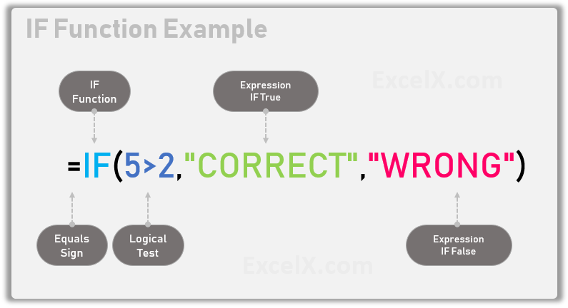
=IF(): Statement to Call Excel IF Function
5>2: is the logical test if 5 is greater than 2
“CORRECT”: value if the logical test returns TRUE
“WRONG”: value if the logical test returns FALSE

Copy the above example and paste in any Cell, this example IF Function returns “CORRECT”.

Example 2: The following example returns “WRONG” based the given expression.

=IF(25=10,”CORRECT”,”WRONG”)

returns “WRONG”

IF Function Checks the first argument (25=10) and it returns FALSE. It will evaluate the third argument (“WRONG”) as it the condition is False.

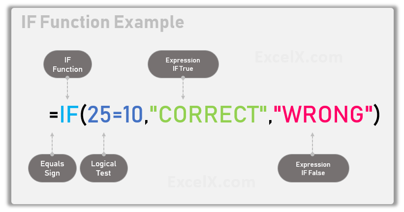
=IF(): Statement to Call Excel IF Function
25=10: is the logical test to check if 25 is equals to 10
“CORRECT”: value if the logical test returns TRUE
“WRONG”: value if the logical test returns FALSE

Copy the above example and paste in any Cell, this example IF Function returns “WRONG”.

Example 3: The following example checks if the given value is even or odd number.

=IF(MOD(25, 2) =0,”Even Number”,”Odd Number”)

returns “Odd Number”

IF Function Checks the first argument [MOD(25, 2) =0] and it returns FALSE. It will evaluate the third argument (“Odd Number”) as it the condition is False.

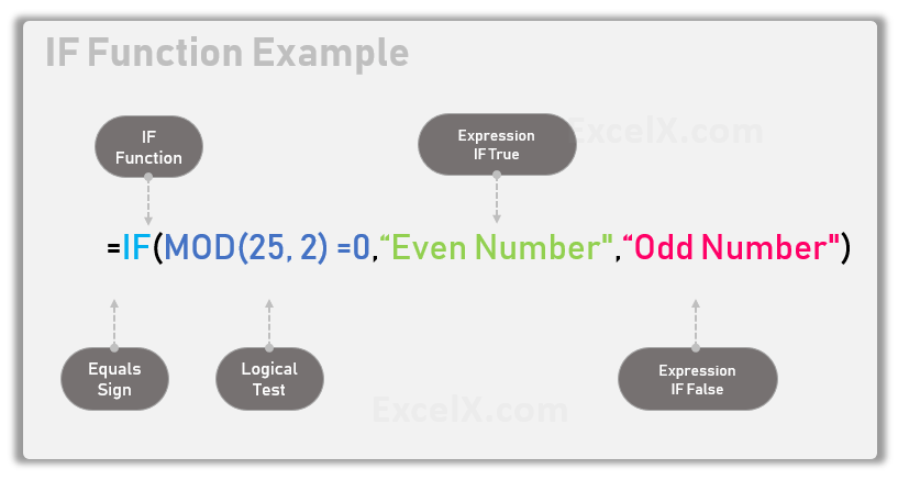
=IF(): Statement to Call Excel IF Function
MOD(25, 2) =0: is the logical test to check if 25 MOD 2 is equals to 0
“Even Number”: value if the logical test returns TRUE
“Odd Number”: value if the logical test returns FALSE

Copy the above example and paste in any Cell, this example IF Function returns “Odd Number”.

Excel IF Function – Practical Examples:

Here are the practical examples of IF Function. IF function is on of the most commonly used Excel Function to check the logical test and nested IF Functions. We can combine the IF Function with Other Excel Function to build the complex expressions and formulas.

IF Function to Compare This Year and Last Year Values:

The following Example shows how to compare the sales values of Current Year and Last Year. We have provide Deparment wise data in the sheet with This Year Data in Column B and This Year Data in Collumn C. And logical test is performed in Column D to check if the Column C values are greater the Column B Values.

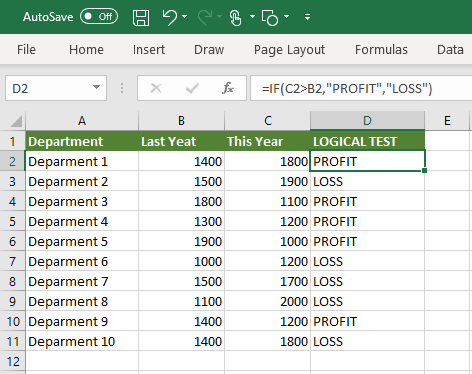
=IF(C2>B2,”PROFIT”,”LOSS”)

IF Function to compare the values in two columns.

You can copy this formula and paste in the Cell D2 and double click to fill the data range.

=IF(): Statement to Call Excel IF Function
C2>B2: is the logical test to check if 25 MOD 2 is equals to 0
“Profit”: value if the logical test returns TRUE
“Loss”: value if the logical test returns FALSE

If Function to Compare Sum of the Column Values

The following IF Formula compare the Sum of Two Columns in Excel Sheet. This will check if Sum of Column C (Range C2:C12) values are greater than Sumn of Column B (Range B2:B12).

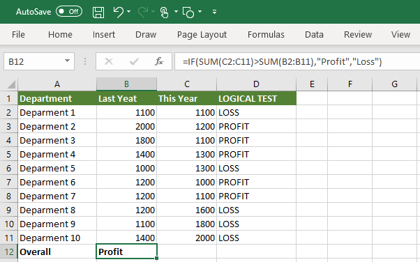
=IF(SUM(C2:C11)>SUM(B2:B11),”Profit”,”Loss”)

IF function to compare sum of two ranges in Excel.

=IF(): Statement to Call Excel IF Function
SUM(C2:C11)>SUM(B2:B11): is the logical test to check if 25 MOD 2 is equals to 0
“Profit”: value if the logical test returns TRUE
“Loss”: value if the logical test returns FALSE

If in Excel have verity of forms and applications. We can use IF formula to check the Boolean condition. We can return some value if the condition is true and some other value if not true or false. Let us see the in-depth details about If in Excel.

If Formula in Excel

We can use the If formula in Excel to check if a condition is meeting certain scenario. For example, we can check if the given value is equals to an integer. We can use If formula to compare two strings. We can return the values based on the Boolean result of If formula in Excel. The following example check if the given value is greater than 10 or not. And return the message based on the result.

=If(25>10,"Given Value is bigger than 10","Given Values is Not Bigger Than 10")

If Formula to check Cell Values

We can check the cell value using If formula and perform the calculations based on the result. Here is a simple example in Cell B1 to check if a cell (A1) is less than or equals to 1000 or not. And add 500 if the values is less than 1000.

=IF(A1<1000,A1+500,A1)

If formula checks the condition (A1<1000) and add 500 if the cell value is less than 1000, it will return the same value if the condition fails.

If Formula to check all values in a Column

We can check the values in a column and perform certain calculation based on the result. Let us see an example to check if any value in column B is equals to zero and flag the respective cell in Column C.

=IF(B1=0,"Zero","")

You can put this formula in C1 and fill-down upto rows of B1.

Share This Story, Choose Your Platform!

4 Comments

Greg
October 29, 2019 at 9:21 am — Reply

Thank you for this easy to understand tutorial on Excel If function. I can say that this is the best way and simple approach to learn IF formula with strong understanding of fundamentals of Excel IF function.
Anna
October 29, 2019 at 9:27 am — Reply

Yes, agree with you!
I am completely impressed with the way of explaining the If function with suitable and real-time examples.

Excellent! Good Job!! Keep it Up!
Jose Valle
June 22, 2022 at 8:58 pm — Reply

how can I make this formula work =MOD(E2-B2-D2+C2,1)*24,IF(G2=”Yes”,F2+0.5,IF(G2=”No”,$F$2)) what I’m I missing or need to do
- PNRao
  July 1, 2022 at 2:50 am — Reply
  
  Comma(,) following number 24. Please describe your question in detailed. Just to inform you, the Mod Value with divisor 1 always return 0.

Page load link

Источник

Simple IF examples

Common problems

Need more help?

See Also

Need more help?

What is IF Function in Excel?

Table of contents

Syntax of the IF Excel Function

How to Use IF Function in Excel?

Example #1

Example #2

Example #3

Example #4

Example #5

Guidelines for the Multiple IF Statements

Frequently Asked Question

IF Excel Function Video

Recommended Articles

Что возвращает функция

Синтаксис

Аргументы функции

Дополнительная информация

Функция Если в Excel примеры с несколькими условиями

Пример 1. Проверяем простое числовое условие с помощью функции IF (ЕСЛИ)

Пример 2. Использование вложенной функции IF (ЕСЛИ) для проверки условия выражения

Пример 3. Вычисляем сумму комиссии с продаж с помощью функции IF (ЕСЛИ) в Excel

Пример 4. Используем логические операторы (AND/OR) (И/ИЛИ) в функции IF (ЕСЛИ) в Excel

Пример 5. Преобразуем ошибки в значения “0” с помощью функции IF (ЕСЛИ)

Introducing IF Function in Excel

1. IF Function

Steps to use IF function in Excel

1. Using the IF function in Excel to identify passed/failed students

2. Nested IF Function

3. IF with AND in Excel

4. IF with OR in Excel

Conclusion

IF Function in Excel

Syntax of IF Function

Simple Examples of Excel IF Function

Excel IF Function – Practical Examples:

IF Function to Compare This Year and Last Year Values:

If Function to Compare Sum of the Column Values

If Formula in Excel

If Formula to check Cell Values

If Formula to check all values in a Column

Share This Story, Choose Your Platform!

4 Comments