
IF function
The IF function is one of the most popular functions in Excel, and it allows you to make logical comparisons between a value and what you expect.
So an IF statement can have two results. The first result is if your comparison is True, the second if your comparison is False.
For example, =IF(C2=”Yes”,1,2) says IF(C2 = Yes, then return a 1, otherwise return a 2).

Use the IF function, one of the logical functions, to return one value if a condition is true and another value if it’s false.
IF(logical_test, value_if_true, [value_if_false])
For example:
-
=IF(A2>B2,»Over Budget»,»OK»)
-
=IF(A2=B2,B4-A4,»»)
|
Argument name |
Description |
|---|---|
|
logical_test (required) |
The condition you want to test. |
|
value_if_true (required) |
The value that you want returned if the result of logical_test is TRUE. |
|
value_if_false (optional) |
The value that you want returned if the result of logical_test is FALSE. |
Simple IF examples

-
=IF(C2=”Yes”,1,2)
In the above example, cell D2 says: IF(C2 = Yes, then return a 1, otherwise return a 2)

-
=IF(C2=1,”Yes”,”No”)
In this example, the formula in cell D2 says: IF(C2 = 1, then return Yes, otherwise return No)As you see, the IF function can be used to evaluate both text and values. It can also be used to evaluate errors. You are not limited to only checking if one thing is equal to another and returning a single result, you can also use mathematical operators and perform additional calculations depending on your criteria. You can also nest multiple IF functions together in order to perform multiple comparisons.

-
=IF(C2>B2,”Over Budget”,”Within Budget”)
In the above example, the IF function in D2 is saying IF(C2 Is Greater Than B2, then return “Over Budget”, otherwise return “Within Budget”)

-
=IF(C2>B2,C2-B2,0)
In the above illustration, instead of returning a text result, we are going to return a mathematical calculation. So the formula in E2 is saying IF(Actual is Greater than Budgeted, then Subtract the Budgeted amount from the Actual amount, otherwise return nothing).

-
=IF(E7=”Yes”,F5*0.0825,0)
In this example, the formula in F7 is saying IF(E7 = “Yes”, then calculate the Total Amount in F5 * 8.25%, otherwise no Sales Tax is due so return 0)
Note: If you are going to use text in formulas, you need to wrap the text in quotes (e.g. “Text”). The only exception to that is using TRUE or FALSE, which Excel automatically understands.
Common problems
|
Problem |
What went wrong |
|---|---|
|
0 (zero) in cell |
There was no argument for either value_if_true or value_if_False arguments. To see the right value returned, add argument text to the two arguments, or add TRUE or FALSE to the argument. |
|
#NAME? in cell |
This usually means that the formula is misspelled. |
Need more help?
You can always ask an expert in the Excel Tech Community or get support in the Answers community.

See Also
IF function — nested formulas and avoiding pitfalls
IFS function
Using IF with AND, OR and NOT functions
COUNTIF function
How to avoid broken formulas
Overview of formulas in Excel
Need more help?
Normally, If you want to write an IF formula for text values in combining with the below two logical operators in excel, such as: “equal to” or “not equal to”.
Table of Contents
- Excel IF function check if a cell contains text(case-insensitive)
- Excel IF function check if a cell contains text (case-sensitive)
- Excel IF function check if part of cell matches specific text
- Excel IF function with Wildcards text value
- Related Formulas
- Related Functions
Excel IF function check if a cell contains text(case-insensitive)
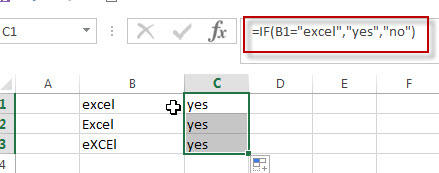
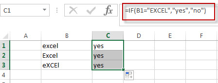
By default, IF function is case-insensitive in excel. It means that the logical text for text values will do not recognize case in the IF formulas. For example, the following two IF formulas will get the same results when checking the text values in cells.
=IF(B1="excel","yes","no")
=IF(B1="EXCEl","yes","no")
The IF formula will check the values of cell B1 if it is equal to “excel” word, If it is TRUE, then return “yes”, otherwise return “no”. And the logical test in the above IF formula will check the text values in the logical_test argument, whatever the logical_test values are “Excel”, “eXcel”, or “EXCEL”, the IF formula don’t care about that if the text values is in lowercase or uppercase, It will get the same results at last.
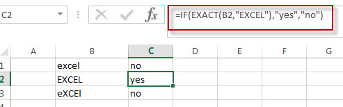
Excel IF function check if a cell contains text (case-sensitive)
If you want to check text values in cells using IF formula in excel (case-sensitive), then you need to create a case-sensitive logical test and then you can use IF function in combination with EXACT function to compare two text values. So if those two text values are exactly the same, then return TRUE. Otherwise return FALSE.
So we can write down the following IF formula combining with EXACT function:
=IF(EXACT(B1,"excel"),"yes","no")
Excel IF function check if part of cell matches specific text
If you want to check if part of text values in cell matches the specific text rather than exact match, to achieve this logic text, you can use IF function in combination with ISNUMBER and SEARCH Function in excel.
Both ISNUMBER and SEARCH functions are case-insensitive in excel.
=IF(ISNUMBER(SEARCH("x",B1)),"good","bad")
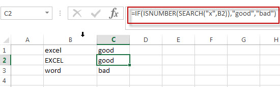
For above the IF formula, it will Check to see if B1 contain the letter x.
Also, we can use FIND function to replace the SEARCH function in the above IF formula. It will return the same results.
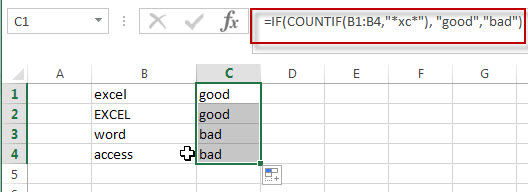
Excel IF function with Wildcards text value
If you wan to use wildcard charcter in an IF formula, for example, if any of the values in column B contains “*xc*”, then return “good”, others return “bad”. You can not directly use the wildcard characters in IF formula, and we can use IF function in combination with COUNTIF function. Let’s see the following IF formula:
=IF(COUNTIF(B1:B4,"*xc*"), "good","bad")
- Excel IF Function With Numbers
If you want to check if a cell values is between two values or checking for the range of numbers or multiple values in cells, at this time, we need to use AND or OR logical function in combination with the logical operator and IF function…
- Excel EXACT function
The Excel SEARCH function returns the number of the starting location of a substring in a text string.The syntax of the EXACT function is as below:= EXACT (text1,text2)… - Excel COUNTIF function
The Excel COUNTIF function will count the number of cells in a range that meet a given criteria.= COUNTIF (range, criteria) … - Excel ISNUMBER function
The Excel ISNUMBER function returns TRUE if the value in a cell is a numeric value, otherwise it will return FALSE. - Excel IF function
The Excel IF function perform a logical test to return one value if the condition is TRUE and return another value if the condition is FALSE…. - Excel SEARCH function
The Excel SEARCH function returns the number of the starting location of a substring in a text string.…
Getting IF Function to Work for Partial Text Match
In the dataset below, we want to write a formula in column B that will search the text in column A. Our formula will search the column A text for the text sequence “AT” and if found display “AT” in column B.

It doesn’t matter where the letters “AT” occur in the column A text, we need to see “AT” in the adjacent cell of column B. If the letters “AT” do not occur in the column A text, the formula in column B should display nothing.
Searching for Text with the IF Function
Let’s begin by selecting cell B5 and entering the following IF formula.
=IF(A5="*AT*","AT","")
Notice the formula returns nothing, even though the text in cell A5 contains the letter sequence “AT”.
The reason it fails is that Excel doesn’t work well when using wildcards directly after an equals sign in a formula.

Any function that uses an equals sign in a logical test does not like to use wildcards in this manner.
“But what about the SUMIFS function?”, I hear you saying.
If you examine a SUMIFS function, the wildcards don’t come directly after the equals sign; they instead come after an argument. As an example:
=SUMIFS($C$4:$C$18,$A$4:$A$18,"*AT*")The wildcard usage does not appear directly after an equals sign.
SEARCH Function to the Rescue
The first thing we need to understand is the syntax of the SEARCH function. The syntax is as follows:
SEARCH(find_text, within_text, [start_num])
- find_text – is a required argument that defines the text you are searching for.
- within_text – is a required argument that defines the text in which you want to search for the value defined in the find_text
- Start_num – is an option argument that defines the character number/position in the within_text argument you wish to start searching. If omitted, the default start character position is 1 (the first character on the left of the text.)
To see if the search function works properly on its own, lets perform a simple test with the following formula.
=SEARCH("AT",A5)
We are returned a character position which the letters “AT” were discovered by the SEARCH function. The first SEARCH found the letters “AT” beginning in the 1st character position of the text. The next discovery was in the 5th character position, and the last discovery was in the 4th character position.
The “#VALUE!” responses are the SEARCH function’s way of letting us know that the letters “AT” were not found in the search text.
We can use this new information to determine if the text “AT” exists in the companion text strings. If we see any number as a response, we know “AT” exists in the text string. If we receive an error response, we know the text “AT” does not exist in the text string.
NOTE: The SEARCH function is NOT case-sensitive. A search for the letters “AT” would find “AT”, “At”, “aT”, and “at”. If you wish to search for text and discriminate between different cases (case-sensitive), use the FIND function. The FIND function works the same as SEARCH, but with the added behavior of case-sensitivity.
Turning Numbers into Decisions
An interesting function in Excel is the ISNUMBER function. The purpose of the ISNUMBER function is to return “True” if something is a number and “False” if something is not a number. The syntax is as follows:
ISNUMBER(value)
- value – is a required argument that defines the data you are examining. The value can refer to a cell, a formula, or a name that refers to a cell, formula, or value.
Let’s add the ISNUMBER function to the logic of our previous SEARCH function.
=ISNUMBER(SEARCH("AT",A5))
Any cell that contained a numeric response is now reading “True” and any cell that contained an error is now reading “False”.
We are now able to use the ISNUMBER/SEARCH functions as our wildcard statement in the original IF function.
=IF(ISNUMBER(SEARCH("AT",A5)),"AT","")
This is a great way to perform logical tests in functions that do not allow for wildcards.
Let’s see another scenario
Suppose we want to search for two different sets of text (“AT” or “DE”) and return the word “Europe” if either of these text strings are discovered in the searched text. We will combine the original formula with an OR function to search for multiple text strings.
=IF(OR(ISNUMBER(SEARCH("AT",A5)),ISNUMBER(SEARCH("DE",A5))),
"Europe","")
Practice Workbook
Feel free to Download the Workbook HERE.
![]()
Published on: June 2, 2019
Last modified: March 29, 2023


Leila Gharani
I’m a 5x Microsoft MVP with over 15 years of experience implementing and professionals on Management Information Systems of different sizes and nature.
My background is Masters in Economics, Economist, Consultant, Oracle HFM Accounting Systems Expert, SAP BW Project Manager. My passion is teaching, experimenting and sharing. I am also addicted to learning and enjoy taking online courses on a variety of topics.
The logical IF statement in Excel is used for the recording of certain conditions. It compares the number and / or text, function, etc. of the formula when the values correspond to the set parameters, and then there is one record, when do not respond — another.
Logic functions — it is a very simple and effective tool that is often used in practice. Let us consider it in details by examples.
The syntax of the function «IF» with one condition
The operation syntax in Excel is the structure of the functions necessary for its operation data.
=IF(boolean;value_if_TRUE;value_if_FALSE)
Let us consider the function syntax:
- Boolean – what the operator checks (text or numeric data cell).
- Value_if_TRUE – what will appear in the cell when the text or numbers correspond to a predetermined condition (true).
- Value_if_FALSE – what appears in the box when the text or the number does not meet the predetermined condition (false).
Example:

Logical IF functions.
The operator checks the A1 cell and compares it to 20. This is a «Boolean». When the contents of the column is more than 20, there is a true legend «greater 20». In the other case it’s «less or equal 20».
Attention! The words in the formula need to be quoted. For Excel to understand that you want to display text values.
Here is one more example. To gain admission to the exam, a group of students must successfully pass a test. The results are listed in a table with columns: a list of students, a credit, an exam.

The statement IF should check not the digital data type but the text. Therefore, we prescribed in the formula В2= «done» We take the quotes for the program to recognize the text correctly.
The function IF in Excel with multiple conditions
Usually one condition for the logic function is not enough. If you need to consider several options for decision-making, spread operators’ IF into each other. Thus, we get several functions IF in Excel.
The syntax is as follows:
Here the operator checks the two parameters. If the first condition is true, the formula returns the first argument is the truth. False — the operator checks the second condition.
Examples of a few conditions of the function IF in Excel:

It’s a table for the analysis of the progress. The student received 5 points:
- А – excellent;
- В – above average or superior work;
- C – satisfactory;
- D – a passing grade;
- E – completely unsatisfactory.
IF statement checks two conditions: the equality of value in the cells.

In this example, we have added a third condition, which implies the presence of another report card and «twos». The principle of the operator is the same.
Enhanced functionality with the help of the operators «AND» and «OR»
When you need to check out a few of the true conditions you use the function И. The point is: IF A = 1 AND A = 2 THEN meaning в ELSE meaning с.
OR function checks the condition 1 or condition 2. As soon as at least one condition is true, the result is true. The point is: IF A = 1 OR A = 2 THEN value B ELSE value C.
Functions AND & OR can check up to 30 conditions.
An example of using the operator AND:

It’s the example of using the logical operator OR.

How to compare data in two tables
Users often need to compare the two spreadsheets in an Excel to match. Examples of the «life»: compare the prices of goods in different bringing, to compare balances (accounting reports) in a few months, the progress of pupils (students) of different classes, in different quarters, etc.
To compare the two tables in Excel, you can use the COUNTIFS statement. Consider the order of application functions.
For example, consider the two tables with the specifications of various food processors. We planned allocation of color differences. This problem in Excel solves the conditional formatting.
Baseline data (tables, which will work with):

Select the first table. Conditional Formatting — create a rule — use a formula to determine the formatted cells:

In the formula bar write: = COUNTIFS (comparable range; first cell of first table)=0. Comparing range is in the second table.
To drive the formula into the range, just select it first cell and the last. «= 0» means the search for the exact command (not approximate) values.
Choose the format and establish what changes in the cell formula in compliance. It’s better to do a color fill.
Select the second table. Conditional Formatting — create a rule — use the formula. Use the same operator (COUNTIFS). For the second table formula:
Download all examples in Excel

Now it is easy to compare the characteristics of the data in the table.
Skip to content
Рассмотрим использование функции ЕСЛИ в Excel в том случае, если в ячейке находится текст.
- Проверяем условие для полного совпадения текста.
- ЕСЛИ + СОВПАД
- Использование функции ЕСЛИ с частичным совпадением текста.
- ЕСЛИ + ПОИСК
- ЕСЛИ + НАЙТИ
Будьте особо внимательны в том случае, если для вас важен регистр, в котором записаны ваши текстовые значения. Функция ЕСЛИ не проверяет регистр – это делают функции, которые вы в ней используете. Поясним на примере.
Проверяем условие для полного совпадения текста.
Проверку выполнения
доставки организуем при помощи обычного оператора сравнения «=».
=ЕСЛИ(G2=»выполнено»,ИСТИНА,ЛОЖЬ)
При этом будет не важно,
в каком регистре записаны значения в вашей таблице.

Если же вас интересует
именно точное совпадение текстовых значений с учетом регистра, то можно
рекомендовать вместо оператора «=» использовать функцию СОВПАД(). Она проверяет
идентичность двух текстовых значений с учетом регистра отдельных букв.
Вот как это может
выглядеть на примере.

Обратите внимание, что
если в качестве аргумента мы используем текст, то он обязательно должен быть
заключён в кавычки.
ЕСЛИ + СОВПАД
В случае, если нас интересует полное совпадение текста с заданным условием, включая и регистр его символов, то оператор «=» нам не сможет помочь.
Но мы можем использовать функцию СОВПАД (английский аналог — EXACT).
Функция СОВПАД сравнивает два текста и возвращает ИСТИНА в случае их полного совпадения, и ЛОЖЬ — если есть хотя бы одно отличие, включая регистр букв. Поясним возможность ее использования на примере.
Формула проверки выполнения заказа в столбце Н может выглядеть следующим образом:
=ЕСЛИ(СОВПАД(G2,»Выполнено»),»Да»,»Нет»)

Как видите, варианты «ВЫПОЛНЕНО» и «выполнено» не засчитываются как правильные. Засчитываются только полные совпадения. Будет полезно, если важно точное написание текста — например, в артикулах товаров.
Использование функции ЕСЛИ с частичным совпадением текста.
Выше мы с вами
рассмотрели, как использовать текстовые значения в функции ЕСЛИ. Но часто случается,
что необходимо определить не полное, а частичное совпадение текста с каким-то
эталоном. К примеру, нас интересует город, но при этом совершенно не важно его
название.
Первое, что приходит на
ум – использовать подстановочные знаки «?» и «*» (вопросительный знак и
звездочку). Однако, к сожалению, этот простой способ здесь не проходит.
ЕСЛИ + ПОИСК
Нам поможет функция ПОИСК (в английском варианте – SEARCH). Она позволяет определить позицию, начиная с которой искомые символы встречаются в тексте. Синтаксис ее таков:
=ПОИСК(что_ищем, где_ищем, начиная_с_какого_символа_ищем)
Если третий аргумент не
указан, то поиск начинаем с самого начала – с первого символа.
Функция ПОИСК возвращает либо номер позиции, начиная с которой искомые символы встречаются в тексте, либо ошибку.
Но нам для использования в функции ЕСЛИ нужны логические значения.
Здесь нам на помощь приходит еще одна функция EXCEL – ЕЧИСЛО. Если ее аргументом является число, она возвратит логическое значение ИСТИНА. Во всех остальных случаях, в том числе и в случае, если ее аргумент возвращает ошибку, ЕЧИСЛО возвратит ЛОЖЬ.
В итоге наше выражение в
ячейке G2
будет выглядеть следующим образом:
=ЕСЛИ(ЕЧИСЛО(ПОИСК(«город»,B2)),»Город»,»»)
Еще одно важное уточнение. Функция ПОИСК не различает регистр символов.

ЕСЛИ + НАЙТИ
В том случае, если для нас важны строчные и прописные буквы, то придется использовать вместо нее функцию НАЙТИ (в английском варианте – FIND).
Синтаксис ее совершенно аналогичен функции ПОИСК: что ищем, где ищем, начиная с какой позиции.
Изменим нашу формулу в
ячейке G2
=ЕСЛИ(ЕЧИСЛО(НАЙТИ(«город»,B2)),»Да»,»Нет»)

То есть, если регистр символов для вас важен, просто замените ПОИСК на НАЙТИ.
Итак, мы с вами убедились, что простая на первый взгляд функция ЕСЛИ дает нам на самом деле много возможностей для операций с текстом.
[the_ad_group id=»48″]
Примеры использования функции ЕСЛИ:
 Функция ЕСЛИОШИБКА – примеры формул — В статье описано, как использовать функцию ЕСЛИОШИБКА в Excel для обнаружения ошибок и замены их пустой ячейкой, другим значением или определённым сообщением. Покажем примеры, как использовать функцию ЕСЛИОШИБКА с функциями визуального…
  Сравнение ячеек в Excel — Вы узнаете, как сравнивать значения в ячейках Excel на предмет точного совпадения или без учета регистра. Мы предложим вам несколько формул для сопоставления двух ячеек по их значениям, длине или количеству…
 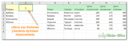 Вычисление номера столбца для извлечения данных в ВПР — Задача: Наиболее простым способом научиться указывать тот столбец, из которого функция ВПР будет извлекать данные. При этом мы не будем изменять саму формулу, поскольку это может привести в случайным ошибкам.…
 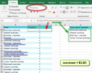 Как проверить правильность ввода данных в Excel? — Подтверждаем правильность ввода галочкой. Задача: При ручном вводе данных в ячейки таблицы проверять правильность ввода в соответствии с имеющимся списком допустимых значений. В случае правильного ввода в отдельном столбце ставить…
 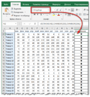 Визуализация данных при помощи функции ЕСЛИ — Функцию ЕСЛИ можно использовать для вставки в таблицу символов, которые наглядно показывают происходящие с данными изменения. К примеру, мы хотим показать в отдельной колонке таблицы, происходит рост или снижение продаж.…
 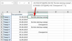 3 примера, как функция ЕСЛИ работает с датами. — На первый взгляд может показаться, что функцию ЕСЛИ для работы с датами можно применять так же, как для числовых и текстовых значений, которые мы только что обсудили. К сожалению, это…