The IF function is one of the most useful Excel functions. It is used to test a condition and return one value if the condition is TRUE and another if it is FALSE.
One of the most common applications of the IF function involves the comparison of values.
These values can be numbers, text, or even dates. However, using the IF statement with date values is not as intuitive as it may seem.
In this tutorial, I will demonstrate some ways in which you can use the IF function with date values.
Syntax and Usage of the IF Function in Excel
The syntax for the IF function is as follows:
IF(logical_test, [value_if_true], [value_if_false])
Here,
- logical_test is the condition or criteria that you want the IF function to test. The result of this parameter is either TRUE or FALSE
- value_if_true is the value that you want the IF function to return if the logical_test evaluates to TRUE
- value_if_false is the value that you want the IF function to return if the logical_test evaluates to FALSE
For example, say you want to write a statement that will return the value “yes” if the value in cell reference A2 is equal to 10, and “no” if it’s anything but 10.
You can then use the following IF function for this scenario:
=IF(A2=10,"yes","no")

Comparing Dates in Excel (Using Operators)
Unlike numbers and strings, comparison operators, when used with dates, have a slightly different meaning.
Here are some of the comparison operators that you can use when comparing dates, along with what they mean:
| Operator | What it Means When Using with Dates |
|---|---|
| < | Before the given date |
| = | Same as the date with which we are comparing |
| > | After the given date |
| <= | Same as or before the given date |
| >= | Same as or after the given date |
It may look like IF formulas for dates are the same as IF functions for numeric or text values, since they use the same comparison operators.
However, it’s not as simple as that.
Unfortunately, unlike other Excel functions, the IF function cannot recognize dates.
It interprets them as regular text values.
So you cannot use a logical test such as “>05/07/2021” in your IF function, as it will simply see the value “05/07/2021” as text.
Here are a few ways in which you can incorporate date values into your IF function’s logical_test parameter.
Using the IF Function with DATEVALUE Function
If you want to use a date in your IF function’s logical test, you can wrap the date in the DATEVALUE function.
This function converts a date in text format to a serial number that Excel can recognize as a date.
If you put a date within quotes, it is essentially a text or string value.
When you pass this as a parameter to the DATEVALUE function, it takes a look at the text inside the double quotes, identifies it as a date and then converts it to an actual Excel date value.
Let us say you have a date in cell A2, and you want cell B2 to display the value “done” if the date comes before or on the same date as “05/07/2021” and display “not done” otherwise.
You can use the IF function along with DATEVALUE in cell B2 as follows:
=IF(A2<DATEVALUE("05/07/2021"),"done","not done")
Here’s a screenshot to illustrate the effect of the above formula:

Using the IF Function with the TODAY Function
If you want to compare a date with the current date, you can use the IF function with the TODAY function in the logical test.
Let’s say you have a date in cell A2 and you want cell B2 to display the value “done” if it is a date before today’s date.
If not, you want let’s say you want to display the value “not done”. You can use the IF function along with the TODAY function in cell B2 as follows:
=IF(A2<TODAY(),"done","not done")
Here’s a screenshot to illustrate the effect of the above formula (assuming the current date is 05/08/2021):

Using the IF Function with Future or Past Dates
An interesting thing about dates in Excel is that you can perform addition and subtraction operations with them too.
This is because dates are basically stored in Excel as serial numbers, starting from the date Jan 1, 1900.
Each day after that is represented by one whole number.
So, the serial number 2 corresponds to Jan 2, 1900, and so on.
This means that adding n number of days to a date is equivalent to adding the value n to the serial number that the date represents.
If TODAY() is 05/07/2021, then TODAY()+5 is five days after today, or 05/12/2021. Similarly, TODAY()-3 is three days before today or 05/04/2021.
Let’s say you have a date in cell A2 and you want cell B2 to mark it as “within range” if it is within 15 days from the current date.
If not, you want to show “out of range”. You can use the IF function along with the TODAY function in cell B2 as follows:
=IF(A2<TODAY()+15,"within range","out of range")
Here’s a screenshot to illustrate the effect of the above formula (assuming the current date is 05/08/2021):

Points to Remember
Having discussed different ways to use dates with the IF function, here are some important points to remember:
- Instead of hardcoding the dates into the IF function’s logical test parameter, you can store the date in a separate cell and refer to it with a cell reference. For example, instead of typing =IF(A2<”05/07/2021”,”done”,”not done”), you can store the date 05/07/2021 in a cell, say B2 and type the formula: =IF(A2<B2,”done”,”not done”).
- Alternatively, you can use the DATEVALUE function as explained in the first part of this tutorial.
- Another neat technique that you can use is to simply add a zero to the date (which has been enclosed in double quotes). So you can type: =IF(A2<”05/07/2021”+0,”done”,”not done”). This will make Excel take the date inside double quotes as a serial number, and use it in the logical test without having its value changed.
In this tutorial, I showed you some great techniques to use the IF function with dates. I hope the tips covered here were useful for you.
Other articles you may also like:
- Multiple If Statements in Excel (Nested Ifs, AND/OR) with Examples
- How to use Excel If Statement with Multiple Conditions Range [AND/OR]
- How to Convert Month Number to Month Name in Excel
- Why are Dates Shown as Hashtags in Excel? Easy Fix!
- How to Convert Serial Numbers to Date in Excel
- How to Get the First Day Of The Month In Excel?
If you have a list of dates and then want to compare to these dates with a specified date to check if those dates is greater than or less than that specified date. You can use the IF function in combination with logical operators and DATEVALUE function in Microsoft excel.
Table of Contents
- Excel IF function combining with DATEVALUE function
- Excel IF function combining with DATE function
- Excel IF function combining with TODAY function
- Related Formulas
- Related Functions
Excel IF function combining with DATEVALUE function
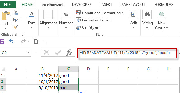
Since that Excel cannot recognize the date formats and just interprets them as a text string. So you need to use DATAVALUE function and let Excel think that it is a Date value. For example: DATEVALUE(“11/3/2018”). Now we can write down the following IF formula with Dates.
=IF(B1<DATEVALUE(“11/3/2018”),”good”,”bad”)
The above excel IF formula will check the date value in Cell B1 if it is less than another specified date(11/3/2018), if the test is TRUE, then return “good”, otherwise return “bad”
Excel IF function combining with DATE function
You can also use DATE function in an Excel IF statement to compare dates, like the below IF formula:
=IF(B1<=DATE(2018,11,3),”good”,””)
The above IF formula will check if the value in cell B1 is less than or equal to 11/3/2018 and show the returned value in cell C1, Otherwise show nothing.
Excel IF function combining with TODAY function
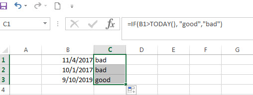
If you want to compare the current date with the specified date in the past, you can use IF function in combination with TODAY function in Excel. Like the following IF formula:
=IF(B1>TODAY(), “good”,”bad”)
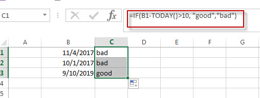
We also can use the complex logical test using Today function, like this: B1-TODAY>10, it will check the date value in one cell if it is more than 10 days from now. Let’s combine this logical test in the IF formula as follow:
=IF(B1-TODAY()>10,”good”,”bad”)
- Excel IF formula with operator : greater than,less than
Now we can use the above logical test with greater than operator. Let’s see the below generic if formula with greater than operator:=IF(A1>10,”excelhow.net”,”google”) … - Excel IF function with text values
If you want to write an IF formula for text values in combining with the below two logical operators in excel, such as: “equal to” or “not equal to”… - Excel IF Function With Numbers
If you want to check if a cell values is between two values or checking for the range of numbers or multiple values in cells, at this time, we need to use AND or OR logical function in combination with the logical operator and IF function…
- Excel Date function
The Excel DATE function returns the serial number for a date.The syntax of the DATE function is as below:= DATE (year, month, day) … - Excel IF function
The Excel IF function perform a logical test to return one value if the condition is TRUE and return another value if the condition is FALSE….
The IF function allows you to make a logical comparison between a value and what you expect by testing for a condition and returning a result if that condition is True or False.
-
=IF(Something is True, then do something, otherwise do something else)
But what if you need to test multiple conditions, where let’s say all conditions need to be True or False (AND), or only one condition needs to be True or False (OR), or if you want to check if a condition does NOT meet your criteria? All 3 functions can be used on their own, but it’s much more common to see them paired with IF functions.
Use the IF function along with AND, OR and NOT to perform multiple evaluations if conditions are True or False.
Syntax
-
IF(AND()) — IF(AND(logical1, [logical2], …), value_if_true, [value_if_false]))
-
IF(OR()) — IF(OR(logical1, [logical2], …), value_if_true, [value_if_false]))
-
IF(NOT()) — IF(NOT(logical1), value_if_true, [value_if_false]))
|
Argument name |
Description |
|
|
logical_test (required) |
The condition you want to test. |
|
|
value_if_true (required) |
The value that you want returned if the result of logical_test is TRUE. |
|
|
value_if_false (optional) |
The value that you want returned if the result of logical_test is FALSE. |
|
Here are overviews of how to structure AND, OR and NOT functions individually. When you combine each one of them with an IF statement, they read like this:
-
AND – =IF(AND(Something is True, Something else is True), Value if True, Value if False)
-
OR – =IF(OR(Something is True, Something else is True), Value if True, Value if False)
-
NOT – =IF(NOT(Something is True), Value if True, Value if False)
Examples
Following are examples of some common nested IF(AND()), IF(OR()) and IF(NOT()) statements. The AND and OR functions can support up to 255 individual conditions, but it’s not good practice to use more than a few because complex, nested formulas can get very difficult to build, test and maintain. The NOT function only takes one condition.
Here are the formulas spelled out according to their logic:
|
Formula |
Description |
|---|---|
|
=IF(AND(A2>0,B2<100),TRUE, FALSE) |
IF A2 (25) is greater than 0, AND B2 (75) is less than 100, then return TRUE, otherwise return FALSE. In this case both conditions are true, so TRUE is returned. |
|
=IF(AND(A3=»Red»,B3=»Green»),TRUE,FALSE) |
If A3 (“Blue”) = “Red”, AND B3 (“Green”) equals “Green” then return TRUE, otherwise return FALSE. In this case only the first condition is true, so FALSE is returned. |
|
=IF(OR(A4>0,B4<50),TRUE, FALSE) |
IF A4 (25) is greater than 0, OR B4 (75) is less than 50, then return TRUE, otherwise return FALSE. In this case, only the first condition is TRUE, but since OR only requires one argument to be true the formula returns TRUE. |
|
=IF(OR(A5=»Red»,B5=»Green»),TRUE,FALSE) |
IF A5 (“Blue”) equals “Red”, OR B5 (“Green”) equals “Green” then return TRUE, otherwise return FALSE. In this case, the second argument is True, so the formula returns TRUE. |
|
=IF(NOT(A6>50),TRUE,FALSE) |
IF A6 (25) is NOT greater than 50, then return TRUE, otherwise return FALSE. In this case 25 is not greater than 50, so the formula returns TRUE. |
|
=IF(NOT(A7=»Red»),TRUE,FALSE) |
IF A7 (“Blue”) is NOT equal to “Red”, then return TRUE, otherwise return FALSE. |
Note that all of the examples have a closing parenthesis after their respective conditions are entered. The remaining True/False arguments are then left as part of the outer IF statement. You can also substitute Text or Numeric values for the TRUE/FALSE values to be returned in the examples.
Here are some examples of using AND, OR and NOT to evaluate dates.
Here are the formulas spelled out according to their logic:
|
Formula |
Description |
|---|---|
|
=IF(A2>B2,TRUE,FALSE) |
IF A2 is greater than B2, return TRUE, otherwise return FALSE. 03/12/14 is greater than 01/01/14, so the formula returns TRUE. |
|
=IF(AND(A3>B2,A3<C2),TRUE,FALSE) |
IF A3 is greater than B2 AND A3 is less than C2, return TRUE, otherwise return FALSE. In this case both arguments are true, so the formula returns TRUE. |
|
=IF(OR(A4>B2,A4<B2+60),TRUE,FALSE) |
IF A4 is greater than B2 OR A4 is less than B2 + 60, return TRUE, otherwise return FALSE. In this case the first argument is true, but the second is false. Since OR only needs one of the arguments to be true, the formula returns TRUE. If you use the Evaluate Formula Wizard from the Formula tab you’ll see how Excel evaluates the formula. |
|
=IF(NOT(A5>B2),TRUE,FALSE) |
IF A5 is not greater than B2, then return TRUE, otherwise return FALSE. In this case, A5 is greater than B2, so the formula returns FALSE. |
Using AND, OR and NOT with Conditional Formatting
You can also use AND, OR and NOT to set Conditional Formatting criteria with the formula option. When you do this you can omit the IF function and use AND, OR and NOT on their own.
From the Home tab, click Conditional Formatting > New Rule. Next, select the “Use a formula to determine which cells to format” option, enter your formula and apply the format of your choice.
Using the earlier Dates example, here is what the formulas would be.
|
Formula |
Description |
|---|---|
|
=A2>B2 |
If A2 is greater than B2, format the cell, otherwise do nothing. |
|
=AND(A3>B2,A3<C2) |
If A3 is greater than B2 AND A3 is less than C2, format the cell, otherwise do nothing. |
|
=OR(A4>B2,A4<B2+60) |
If A4 is greater than B2 OR A4 is less than B2 plus 60 (days), then format the cell, otherwise do nothing. |
|
=NOT(A5>B2) |
If A5 is NOT greater than B2, format the cell, otherwise do nothing. In this case A5 is greater than B2, so the result will return FALSE. If you were to change the formula to =NOT(B2>A5) it would return TRUE and the cell would be formatted. |
Note: A common error is to enter your formula into Conditional Formatting without the equals sign (=). If you do this you’ll see that the Conditional Formatting dialog will add the equals sign and quotes to the formula — =»OR(A4>B2,A4<B2+60)», so you’ll need to remove the quotes before the formula will respond properly.
Need more help?

See also
You can always ask an expert in the Excel Tech Community or get support in the Answers community.
Learn how to use nested functions in a formula
IF function
AND function
OR function
NOT function
Overview of formulas in Excel
How to avoid broken formulas
Detect errors in formulas
Keyboard shortcuts in Excel
Logical functions (reference)
Excel functions (alphabetical)
Excel functions (by category)
Skip to content
На первый взгляд может показаться, что функцию ЕСЛИ для работы с датами можно применять так же, как для числовых и текстовых значений, которые мы только что обсудили. К сожалению, это не так.
Примеры работы функции ЕСЛИ с датами.
Дата в качестве условия, с которым работает функция ЕСЛИ, может быть записана в какую-то ячейку Excel, либо же прямо вставлена в формулу. Вот тут-то и возникают некоторые особенности и сложности работы функции ЕСЛИ с датами.
Пример 1. Формула условия для дат с
функцией ДАТАЗНАЧ (DATEVALUE)
Иногда случается, что записать дату непосредственно в функцию ЕСЛИ, не ссылаясь ни на какую ячейку. В этом случае возникают некоторые сложности.
В отличие от многих
других функций Excel, ЕСЛИ не может распознавать даты и интерпретирует их как текст,
как простые текстовые строки.
Поэтому вы не можете выразить свое логическое условие просто как >«15.07.2019» или же >15.07.2019. Увы, ни один из приведенных вариантов не верен.
Чтобы функция ЕСЛИ распознала дату в вашем логическом условии именно как дату, вы должны обернуть ее в функцию ДАТАЗНАЧ (в английском варианте – DATEVALUE).
Например, ДАТАЗНАЧ(«15.07.2019»).
Полная формула ЕСЛИ может
иметь следующую форму:
=ЕСЛИ(B2<ДАТАЗНАЧ(«10.09.2019″),»Поступил»,»Ожидается»)
Как показано на скриншоте,
эта формула ЕСЛИ оценивает даты в столбце В и возвращает «Послупил», если дата
поступления до 10 сентября. В противном случае формула возвращает «Ожидается».
Пример 2. Формула условия для дат с
функцией СЕГОДНЯ()
В случае, когда даты записаны в ячейки таблицы Excel, применять ДАТАЗНАЧ нет необходимости.
Если вы основываете свое условие на текущей дате, то можете взять функцию СЕГОДНЯ (в английском варианте — TODAY) в качестве аргумента функции ЕСЛИ.
К примеру, сегодня — 9 сентября 2019 года.
В столбце C отметим товар, который уже поступил. В ячейке C2 запишем:
=ЕСЛИ(B2<СЕГОДНЯ(),»Поступил»,»»)
В столбце D отметим товар, который еще не поступил. В ячейке D2 запишем:
=ЕСЛИ(B2<СЕГОДНЯ(),»»,»Ожидается»)
Пример 3. Расширенные
формулы ЕСЛИ для будущих и прошлых дат
Предположим, вы хотите
отметить только те даты, которые отстоят от текущей более чем на 30 дней.
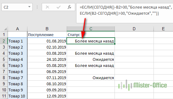
Выделим даты, отстоящие более чем на месяц от текущей, в прошлом. Укажем для них «Более месяца назад». Запишем это условие:
=ЕСЛИ(СЕГОДНЯ()-B2>30,»Более
месяца назад»,»»)
Если условие не выполнено, то в ячейку запишем пустую строку «».
А для будущих дат, также отстоящих более чем на месяц, укажем «Ожидается».
=ЕСЛИ(B2-СЕГОДНЯ()>30,»Ожидается»,»»)
Если все результаты попробовать объединить в одном столбце, то придется составить выражение с несколькими вложенными функциями ЕСЛИ:
=ЕСЛИ(СЕГОДНЯ()-B2>30,»Более месяца назад», ЕСЛИ(B2-СЕГОДНЯ()>30,»Ожидается»,»»))
Примеры работы функции ЕСЛИ:
Return to Excel Formulas List
Download Example Workbook
Download the example workbook
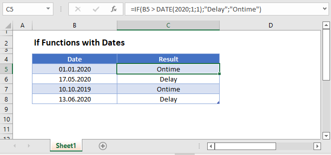
This tutorial will demonstrate how to use the IF Function with Dates in Excel and Google Sheets.
IF & DATE Functions
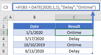
To use dates within IF Functions, you can use the DATE Function to define a date:
=IF(B3 > DATE(2020,1,1),"Delay","Ontime")One example of this formula is to calculate if a payment is over due:
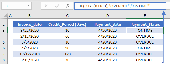
Payment Over Due
=IF(D3>=(B3+C3),"OVERDUE","ONTIME")If Function with Dates – Google Sheets
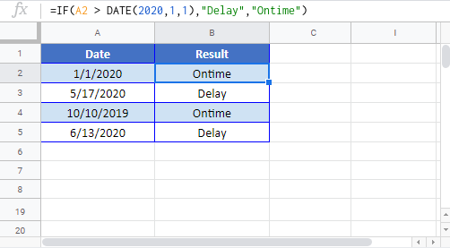
All of the above examples work exactly the same in Google Sheets as in Excel.


