If function excel any number

IF function

The IF function is one of the most popular functions in Excel, and it allows you to make logical comparisons between a value and what you expect.

So an IF statement can have two results. The first result is if your comparison is True, the second if your comparison is False.

For example, =IF(C2=”Yes”,1,2) says IF(C2 = Yes, then return a 1, otherwise return a 2).

Use the IF function, one of the logical functions, to return one value if a condition is true and another value if it’s false.

IF(logical_test, value_if_true, [value_if_false])

For example:

• =IF(A2>B2,»Over Budget»,»OK»)

• =IF(A2=B2,B4-A4,»»)

Argument name	Description
logical_test    (required)	The condition you want to test.
value_if_true    (required)	The value that you want returned if the result of logical_test is TRUE.
value_if_false    (optional)	The value that you want returned if the result of logical_test is FALSE.

Simple IF examples

• =IF(C2=”Yes”,1,2)

In the above example, cell D2 says: IF(C2 = Yes, then return a 1, otherwise return a 2)

• =IF(C2=1,”Yes”,”No”)

In this example, the formula in cell D2 says: IF(C2 = 1, then return Yes, otherwise return No)As you see, the IF function can be used to evaluate both text and values. It can also be used to evaluate errors. You are not limited to only checking if one thing is equal to another and returning a single result, you can also use mathematical operators and perform additional calculations depending on your criteria. You can also nest multiple IF functions together in order to perform multiple comparisons.

• =IF(C2>B2,”Over Budget”,”Within Budget”)

In the above example, the IF function in D2 is saying IF(C2 Is Greater Than B2, then return “Over Budget”, otherwise return “Within Budget”)

• =IF(C2>B2,C2-B2,0)

In the above illustration, instead of returning a text result, we are going to return a mathematical calculation. So the formula in E2 is saying IF(Actual is Greater than Budgeted, then Subtract the Budgeted amount from the Actual amount, otherwise return nothing).

• =IF(E7=”Yes”,F5*0.0825,0)

In this example, the formula in F7 is saying IF(E7 = “Yes”, then calculate the Total Amount in F5 * 8.25%, otherwise no Sales Tax is due so return 0)

Note: If you are going to use text in formulas, you need to wrap the text in quotes (e.g. “Text”). The only exception to that is using TRUE or FALSE, which Excel automatically understands.

Common problems

Problem	What went wrong
0 (zero) in cell	There was no argument for either value_if_true or value_if_False arguments. To see the right value returned, add argument text to the two arguments, or add TRUE or FALSE to the argument.
#NAME? in cell	This usually means that the formula is misspelled.

Need more help?

You can always ask an expert in the Excel Tech Community or get support in the Answers community.

See Also

IF function — nested formulas and avoiding pitfalls

IFS function

Using IF with AND, OR and NOT functions

COUNTIF function

How to avoid broken formulas

Overview of formulas in Excel

This tutorial demonstrates how to check if a cell contains any number in Excel and Google Sheets.

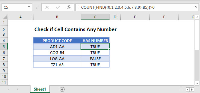
Cell Contains Any Number

In Excel, if a cell contains numbers and letters, the cell is considered a text cell. You can check if a text cell contains any number by using the COUNT and FIND Functions.

=COUNT(FIND({0,1,2,3,4,5,6,7,8,9},B3))>0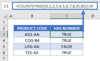

The formula above checks for the digits 0–9 in a cell and counts the number of discrete digits the cell contains. Then it returns TRUE if the count is positive or FALSE if it is zero.

Let’s step through each function below to understand this example.

FIND a Number in a Cell

First, we use the FIND Function. The FIND Function finds the position of a character within a text string.

=FIND({0,1,2,3,4,5,6,7,8,9},B3)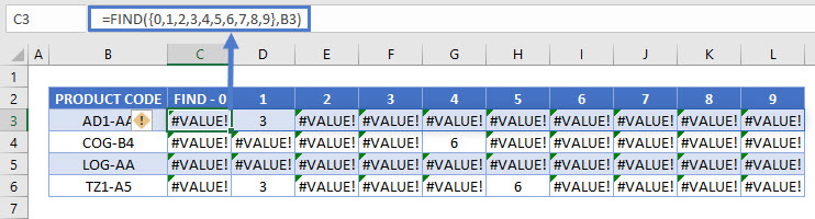

In this example, we use an array of all numerical characters (digits 0–9) and find each one in the cell. Since our input is an array – in curly brackets {} – our output is also an array. The example above shows how the FIND Function is performed ten times on each cell (once for each numerical digit).

If the number is found, it’s position is output. Above you can see the number “1” is found in the 3rd position in the first row and “4” is found in the 6th position in the 2nd row.

If a number is not found, the #VALUE! Error is displayed.

Note: The FIND and SEARCH Functions return the same result when used to search for numbers. Either function can be used.

COUNT the Number of Digits

Next, we count the non-error outputs from the last step. The COUNT Function counts the number of numeric values found in the array, ignoring errors.

=COUNT(C3:L3)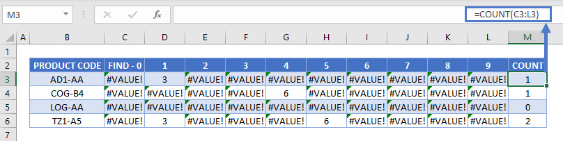

Test the Number Count

Finally, we need to test whether the result from the last step is greater than zero. The formula below returns TRUE for non-zero counts (where the target cell contains a number) and FALSE for any zero counts.

=M3>0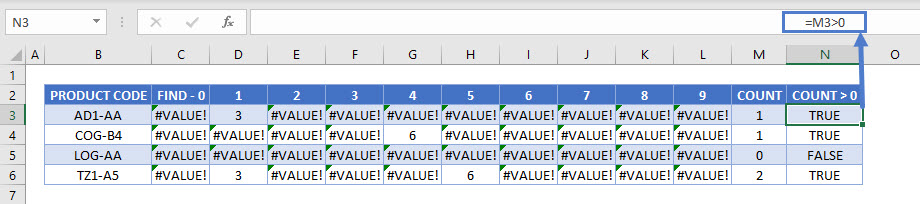

Combining these steps gives us our initial formula:

=COUNT(FIND({0,1,2,3,4,5,6,7,8,9},B3))>0

Check if Cell Contains Specific Number

To check if a cell contains a specific number, we can use the FIND or SEARCH Function.

=FIND(5,B3)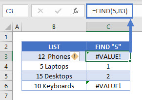

In this example we use the FIND Function to check for the number 5 in column B. It returns the position of the number 5 in the cell if it is found and a VALUE error if “5” is not found.

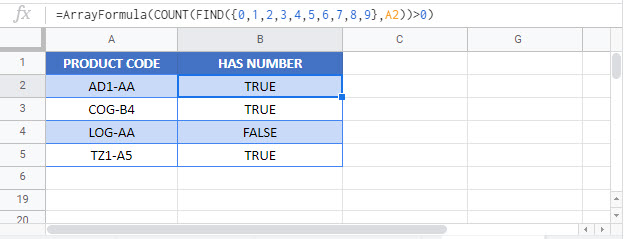
Check if Cell Contains Any Number – Google Sheets

These formulas work the same in Google Sheets as in Excel. However, you need to press CTRL + SHIFT + ENTER for Google Sheets to recognize an array formula.

Alternatively, you could type “ArrayFormula” and put the formula in parentheses. Both methods produce the same result.

The IF function runs a logical test and returns one value for a TRUE result, and another value for a FALSE result. The result from IF can be a value, a cell reference, or even another formula. By combining the IF function with other logical functions like AND and OR, you can test more than one condition at a time.

Syntax

The generic syntax for the IF function looks like this:

=IF(logical_test,[value_if_true],[value_if_false])

The first argument, logical_test, is typically an expression that returns either TRUE or FALSE. The second argument, value_if_true, is the value to return when logical_test is TRUE. The last argument, value_if_false, is the value to return when logical_test is FALSE. Both value_if_true and value_if_false are optional, but you must provide one or the other. For example, if cell A1 contains 80, then:

=IF(A1>75,TRUE) // returns TRUE
=IF(A1>75,"OK") // returns "OK"
=IF(A1>85,"OK") // returns FALSE
=IF(A1>75,10,0) // returns 10
=IF(A1>85,10,0) // returns 0
=IF(A1>75,"Yes","No") // returns "Yes"
=IF(A1>85,"Yes","No") // returns "No"

Notice that text values like «OK», «Yes», «No», etc. must be enclosed in double quotes («»). However, numeric values should not be enclosed in quotes.

Logical tests

The IF function supports logical operators (>,<,<>,=) when creating logical tests. Most commonly, the logical_test in IF is a complete logical expression that will evaluate to TRUE or FALSE. The table below shows some common examples:

Goal	Logical test
If A1 is greater than 75	A1>75
If A1 equals 100	A1=100
If A1 is less than or equal to 100	A1<=100
If A1 equals «Red»	A1=»red»
If A1 is not equal to «Red»	A1<>»red»
If A1 is less than B1	A1<B1
If A1 is empty	A1=»»
If A1 is not empty	A1<>»»
If A1 is less than current date	A1<TODAY()

Notice text values must be enclosed in double quotes («»), but numbers do not. The IF function does not support wildcards, but you can combine IF with COUNTIF to get basic wildcard functionality. To test for substrings in a cell, you can use the IF function with the SEARCH function.

Pass or Fail example

In the worksheet shown above, we want to assign either «Pass» or «Fail» based on a test score. A passing score is 70 or higher. The formula in D6, copied down, is:

=IF(C5>=70,"Pass","Fail")

Translation: If the value in C5 is greater than or equal to 70, return «Pass». Otherwise, return «Fail».

Note that the logical flow of this formula can be reversed. This formula returns the same result:

=IF(C5<70,"Fail","Pass")

Translation: If the value in C5 is less than 70, return «Fail». Otherwise, return «Pass».

Both formulas above, when copied down, will return correct results.

Note: If you are new to the idea of formula criteria, this article explains many examples.

Assign points based on color

In the worksheet below, we want to assign points based on the color in column B. If the color is «red», the result should be 100. If the color is «blue», the result should be 125. This requires that we use a formula based on two IF functions, one nested inside the other. The formula in C5, copied down, is:

=IF(B5="red",100,IF(B5="blue",125))

Translation: IF the value in B5 is «red», return 100. Else, if the value in B5 is «blue», return 125.

There are three things to notice in this example:

1. The formula will return FALSE if the value in B5 is anything except «red» or «blue»
2. The text values «red» and «blue» must be enclosed in double quotes («»)
3. The IF function is not case-sensitive and will match «red», «Red», «RED», or «rEd».

This is a simple example of a nested IFs formula. See below for a more complex example.

Return another formula

The IF function can return another formula as a result. For example, the formula below will return A1*5% when A1 is less than 100, and A1*7% when A1 is greater than or equal to 100:

=IF(A1<100,A1*5%,A1*7%)

Nested IF statements

The IF function can be «nested». A «nested IF» refers to a formula where at least one IF function is nested inside another in order to test for more conditions and return more possible results. Each IF statement needs to be carefully «nested» inside another so that the logic is correct. For example, the following formula can be used to assign a grade rather than a pass / fail result:

=IF(C6<70,"F",IF(C6<75,"D",IF(C6<85,"C",IF(C6<95,"B","A"))))

Up to 64 IF functions can be nested. However, in general, you should consider other functions, like VLOOKUP or XLOOKUP for more complex scenarios, because they can handle more conditions in a more streamlined fashion. For a more details see this article on nested IFs.

Note: the newer IFS function is designed to handle multiple conditions without nesting. However, a lookup function like VLOOKUP or XLOOKUP is usually a better approach unless the logic for each condition is custom.

IF with AND, OR, NOT

The IF function can be combined with the AND function and the OR function. For example, to return «OK» when A1 is between 7 and 10, you can use a formula like this:

=IF(AND(A1>7,A1<10),"OK","")

Translation: if A1 is greater than 7 and less than 10, return «OK». Otherwise, return nothing («»).

To return B1+10 when A1 is «red» or «blue» you can use the OR function like this:

=IF(OR(A1="red",A1="blue"),B1+10,B1)

Translation: if A1 is red or blue, return B1+10, otherwise return B1.

=IF(NOT(A1="red"),B1+10,B1)

Translation: if A1 is NOT red, return B1+10, otherwise return B1.

IF cell contains specific text

Because the IF function does not support wildcards, it is not obvious how to configure IF to check for a specific substring in a cell. A common approach is to combine the ISNUMBER function and the SEARCH function to create a logical test like this:

=ISNUMBER(SEARCH(substring,A1)) // returns TRUE or FALSE

For example, to check for the substring «xyz» in cell A1, you can use a formula like this:

=IF(ISNUMBER(SEARCH("xyz",A1)),"Yes","No")

Read a detailed explanation here.

More information

• Read more about nested IFs
• Learn how to use VLOOKUP instead of nested IFs (video)
• 50 Examples of formula criteria

Notes

• The IF function is not case-sensitive.
• To count values conditionally, use the COUNTIF or the COUNTIFS functions.
• To sum values conditionally, use the SUMIF or the SUMIFS functions.
• If any of the arguments to IF are supplied as arrays, the IF function will evaluate every element of the array.

Normally, If you want to write an IF formula for numbers in combining with the  logical operators in excel, such as: greater than, less than, greater than or equal to, less than or equal to, equal to, not equal to.etc.

The generic IF formula with logical operator for number values is as below:

=IF(B1>10,”good”,”bad”)

Excel IF formula for range of numbers

If you want to check if a cell values is between two values or checking for the range of numbers or multiple values in cells, at this time, we need to use AND or OR logical function in combination with the logical operator and IF function.

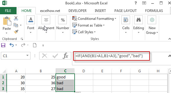
For example, you need to check if the value in cell B1 is between values in Cell A1 and A3, then we can write down the following excel IF formula:

=IF(AND(B1>A1,B1<A3),"good","bad")

We can enter the above formula into the formula bar in the cell C1 and then press the Enter key. And rag the Fill Handle to the range C1:C3.it will apply for the other cells for this formula.

Excel IF formula for negative numbers

If you want to create an IF formula to display some text string in cells if the value in cell falls between the range negative numbers -10 to positive numbers 10.

Actually, whatever negative numbers or positive numbers, we still can use AND or OR logical function to create a logical test in IF formula. we can write down the following IF formula:

=IF(AND(B1>-10, B1<10),”good”,”bad”)

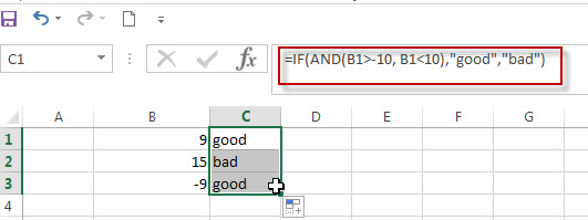
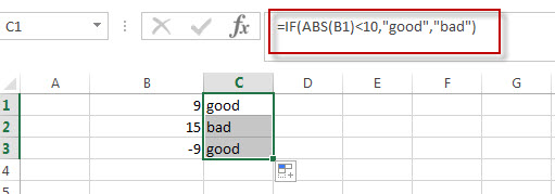
Also, we can use another excel function ABS() to achieve the same results. Let’s see the below IF formula in combination with ABS function.

=IF(ABS(B1)<10,”good”,”bad”)

---

• Excel IF formula with operator : greater than,less than
  Now we can use the above logical test with greater than operator. Let’s see the below generic if formula with greater than operator:=IF(A1>10,”excelhow.net”,”google”) …
  
• Excel IF function with text values
  If you want to write an IF formula for text values in combining with the below two logical operators in excel, such as: “equal to” or “not equal to”.
• Excel IF function with Dates 
  If you have a list of dates and then want to compare to these dates with a specified date to check if those dates is greater than or less than that specified date. …
• Excel IF Function With Numbers
  If you want to check if a cell values is between two values or checking for the range of numbers or multiple values in cells, at this time, we need to use AND or OR logical function in combination with the logical operator and IF function…

• Excel AND function
  The Excel AND function returns TRUE if all of arguments are TRUE, and it returns FALSE if any of arguments are FALSE.The syntax of the AND function is as below:= AND (condition1,[condition2],…) …
• Excel IF function 
  The Excel IF function perform a logical test to return one value if the condition is TRUE and return another value if the condition is FALSE….
• Excel nested if function
  The nested IF function is formed by multiple if statements within one Excel if function. This excel nested if statement makes it possible for a single formula to take multiple actions…
• Excel ABS function
  The Excel ABS function returns the absolute value of a number

Excel IF Function – Introduction

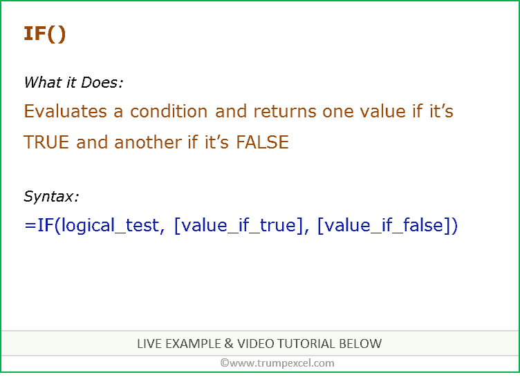
When to use Excel IF Function

IF function in Excel is best suited for situations where you check whether a condition is TRUE or FALSE. If it’s TRUE, the function returns a specified value/reference, and if not then it returns another specified value/reference.

What it Returns

It returns whatever value you specify for the TRUE or FALSE condition.

Syntax

=IF(logical_test, [value_if_true], [value_if_false])

Input Arguments

• logical_test – this is the condition that you want to test. It could be a logical expression that can evaluate to TRUE or FALSE. This can either be a cell reference, a result of some other formula, or can be manually entered.
• [value_if_true] – (Optional) This is the value that is returned when the logical_test evaluates to TRUE.
• [value_if_false] – (Optional) This is the value that is returned when the logical_test evaluates to FALSE.

Important Notes About using IF Function in Excel

• A maximum of 64 nested IF conditions can be tested in the formula.
• If any of the argument is an array, each element of the array is evaluated.
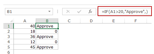
• If you omit the FALSE argument (value_if_false), i.e., there is only a comma after the  value_if_true argument, the function would return a 0 when the condition is FALSE.
  • For example, in the example below, the formula is =IF(A1>20,”Approve”,), where the value_if_false is not specified, however, the value_if_true argument is still followed by a comma. This would return 0 whenever the checked condition is not met.
• If you omit the TRUE argument (value_if_true), and specify only the value_if_false argument, the function would return a 0 when the condition is TRUE.
  • For example, in the example below, the formula is =IF(A1>20,,”Approve”), where the value_if_true is not specified (only a comma is used to then specify the value_if_false value). This would return 0 whenever the checked condition is met.

Excel IF Function – Examples

Here are five practical examples of using the IF function in Excel.

Example 1: Using Excel IF function to Check a Simple Numeric Condition

When using Excel IF function with numbers, you can use a variety of operators to check a condition. Here is a list of operators you can use:

Below is a simple example where students marks are checked. If the marks are more than or equal to 35, the function returns Pass, else it returns Fail.

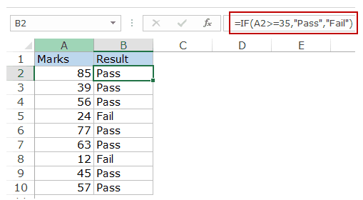
Example 2: Using Nested IF to Check a Sequence of Conditions

Excel IF Function can take up to 64 conditions at once. While it’s inadvisable to create long Nested IF functions, in the case of limited conditions, you can create a formula that checks conditions in a sequence.

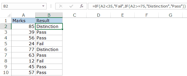
In the example below, we check for two conditions.

• The first condition checks whether the marks are less than 35. If this is TRUE it returns Fail.
• In case the first condition is FALSE, which means that the student scored above or equal to 35, it checks for another condition. It checks if the marks are greater than or equal to 75. If this is true, it returns Distinction, else it simply returns Pass.

Example 3: Calculating Commissions Using Excel IF Function

Excel If Function allows you to perform calculations in the value section. A good example of this is calculating the sales commission for sales rep using the IF function.

In the example below, a sales rep gets no commission if the sales are less than 50K, gets a 2% commission if the sales are between 50-100K and 4% commission if the sales are more than 100K.

Here is the formula used:

=IF(B2<50,0,If(B2<100,B2*2%,B2*4%))

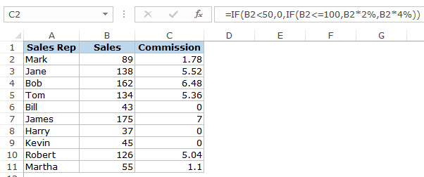
In the formula used in the example above, the calculation is done within the IF function itself. When the sales value is between 50-100K, it returns B2*2%, which is the 2% commission based on the sales value.

Example 4: Using Logical Operators (AND/OR) in Excel IF Function

You can use logical operators (AND/OR) within the IF function to test multiple conditions at once.

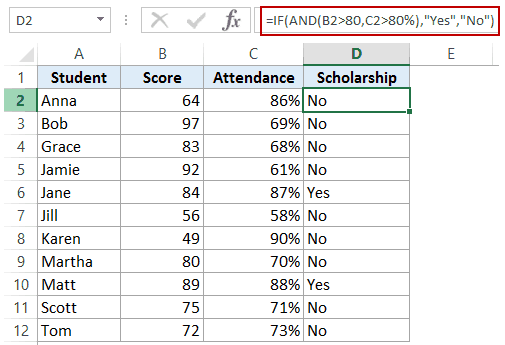
For example, suppose you’ve to select students for the scholarship based on marks and attendance. In the example shown below, a student is eligible only if he scores more than 80 and has the attendance of more than 80%.

You can use the AND function within the IF function to first check whether both these conditions are met or not. If the conditions are met, the function returns Eligible, else it returns Not Eligible.

Here is the formula that will do this:

=IF(AND(B2>80,C2>80%),”Yes”,”No”)

Example 5: Converting all Errors to Zero using Excel IF function

Excel IF function can also be used to get rid of cells that contain errors. You can convert the error values to blanks or zeros or any other value.

Here is the formula that will do it:

=IF(ISERROR(A1),0,A1)

The formula returns a 0 when there is an error value, else it returns the value in the cell.

NOTE: If you’re using Excel 2007 or versions after it, you can also use the IFERROR function to do this. 

Similarly, you can also handle blank cells. In case of blank cells, use the ISBLANK function as shown below:

=IF(ISBLANK(A1),0,A1)

Excel IF Function – Video Tutorial

Related Excel Functions:

• Excel AND Function.
• Excel OR Function.
• Excel NOT Function.
• Excel IFS Function.
• Excel IFERROR Function.
• Excel FALSE Function.
• Excel TRUE Function

Other Excel tutorials you may find useful:

• Avoid Nested IF Function in Excel by using VLOOKUP