If formula in excel with list - Word и Excel - помощь в работе с программами

So, there are times when you would like to know that a value is in a list or not. We have done this using VLOOKUP. But we can do the same thing using COUNTIF function too. So in this article, we will learn how to check if a values is in a list or not using various ways.

Check If Value In Range Using COUNTIF Function

So as we know, using COUNTIF function in excel we can know how many times a specific value occurs in a range. So if we count for a specific value in a range and its greater than zero, it would mean that it is in the range. Isn’t it?

Generic Formula

=COUNTIF(range,value)>0

Range: The range in which you want to check if the value exist in range or not.

Value: The value that you want to check in the range.

Let’s see an example:

Excel Find Value is in Range Example

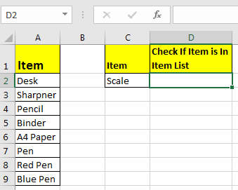
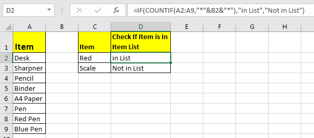
For this example, we have below sample data. We need a check-in the cell D2, if the given item in C2 exists in range A2:A9 or say item list. If it’s there then, print TRUE else FALSE.

Write this formula in cell D2:

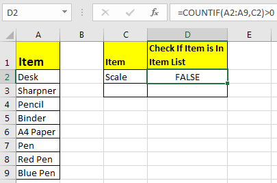
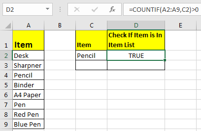
Since C2 contains “scale” and it’s not in the item list, it shows FALSE. Exactly as we wanted. Now if you replace “scale” with “Pencil” in the formula above, it’ll show TRUE.

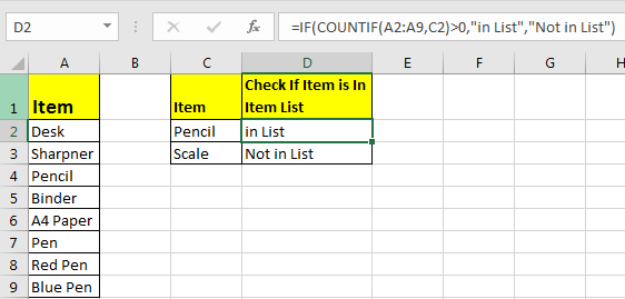
Now, this TRUE and FALSE looks very back and white. How about customizing the output. I mean, how about we show, “found” or “not found” when value is in list and when it is not respectively.
Since this test gives us TRUE and FALSE, we can use it with IF function of excel.

Write this formula:

=IF(COUNTIF(A2:A9,C2)>0,»in List»,»Not in List»)

You will have this as your output.

What If you remove “>0” from this if formula?

=IF(COUNTIF(A2:A9,C2),»in List»,»Not in List»)

It will work fine. You will have same result as above. Why? Because IF function in excel treats any value greater than 0 as TRUE.

How to check if a value is in Range with Wild Card Operators

Sometimes you would want to know if there is any match of your item in the list or not. I mean when you don’t want an exact match but any match.

For example, if in the above-given list, you want to check if there is anything with “red”. To do so, write this formula.

=IF(COUNTIF(A2:A9,»*red*»),»in List»,»Not in List»)

This will return a TRUE since we have “red pen” in our list. If you replace red with pink it will return FALSE. Try it.
Now here I have hardcoded the value in list but if your value is in a cell, say in our favourite cell B2 then write this formula.

IF(COUNTIF(A2:A9,»*»&B2&»*»),»in List»,»Not in List»)

There’s one more way to do the same. We can use the MATCH function in excel to check if the column contains a value. Let’s see how.

Find if a Value is in a List Using MATCH Function

So as we all know that MATCH function in excel returns the index of a value if found, else returns #N/A error. So we can use the ISNUMBER to check if the function returns a number.
If it returns a number ISNUMBER will show TRUE, which means it’s found else FALSE, and you know what that means.

Write this formula in cell C2:

=ISNUMBER(MATCH(C2,A2:A9,0))

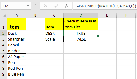
The MATCH function looks for an exact match of value in cell C2 in range A2:A9. Since DESK is on the list, it shows a TRUE value and FALSE for SCALE.

So yeah, these are the ways, using which you can find if a value is in the list or not and then take action on them as you like using IF function. I explained how to find value in a range in the best way possible. Let me know if you have any thoughts. The comments section is all yours.

Related Articles:

How to Check If Cell Contains Specific Text in Excel

How to Check A list of Texts In String in Excel

How to take the Average Difference between lists in Excel

How to Get Every Nth Value From A list in Excel

Popular Articles:

50 Excel Shortcuts to Increase Your Productivity

How to use the VLOOKUP Function in Excel

How to use the COUNTIF function in Excel

How to use the SUMIF Function in Excel

Источник

IF function

The IF function is one of the most popular functions in Excel, and it allows you to make logical comparisons between a value and what you expect.

So an IF statement can have two results. The first result is if your comparison is True, the second if your comparison is False.

For example, =IF(C2=”Yes”,1,2) says IF(C2 = Yes, then return a 1, otherwise return a 2).

Use the IF function, one of the logical functions, to return one value if a condition is true and another value if it’s false.

IF(logical_test, value_if_true, [value_if_false])

For example:

=IF(A2>B2,»Over Budget»,»OK»)
=IF(A2=B2,B4-A4,»»)

Argument name	Description
logical_test (required)	The condition you want to test.
value_if_true (required)	The value that you want returned if the result of *logical_test* is TRUE.
value_if_false (optional)	The value that you want returned if the result of *logical_test* is FALSE.

Simple IF examples

=IF(C2=”Yes”,1,2)

In the above example, cell D2 says: IF(C2 = Yes, then return a 1, otherwise return a 2)

=IF(C2=1,”Yes”,”No”)

In this example, the formula in cell D2 says: IF(C2 = 1, then return Yes, otherwise return No)As you see, the IF function can be used to evaluate both text and values. It can also be used to evaluate errors. You are not limited to only checking if one thing is equal to another and returning a single result, you can also use mathematical operators and perform additional calculations depending on your criteria. You can also nest multiple IF functions together in order to perform multiple comparisons.

=IF(C2>B2,”Over Budget”,”Within Budget”)

In the above example, the IF function in D2 is saying IF(C2 Is Greater Than B2, then return “Over Budget”, otherwise return “Within Budget”)

=IF(C2>B2,C2-B2,0)

In the above illustration, instead of returning a text result, we are going to return a mathematical calculation. So the formula in E2 is saying IF(Actual is Greater than Budgeted, then Subtract the Budgeted amount from the Actual amount, otherwise return nothing).

=IF(E7=”Yes”,F5*0.0825,0)

In this example, the formula in F7 is saying IF(E7 = “Yes”, then calculate the Total Amount in F5 * 8.25%, otherwise no Sales Tax is due so return 0)

Note: If you are going to use text in formulas, you need to wrap the text in quotes (e.g. “Text”). The only exception to that is using TRUE or FALSE, which Excel automatically understands.

Common problems

Problem	What went wrong
0 (zero) in cell	There was no argument for either value_if_true or value_if_False arguments. To see the right value returned, add argument text to the two arguments, or add TRUE or FALSE to the argument.
#NAME? in cell	This usually means that the formula is misspelled.

Need more help?

You can always ask an expert in the Excel Tech Community or get support in the Answers community.

1. Check if the cell contains any value in the list

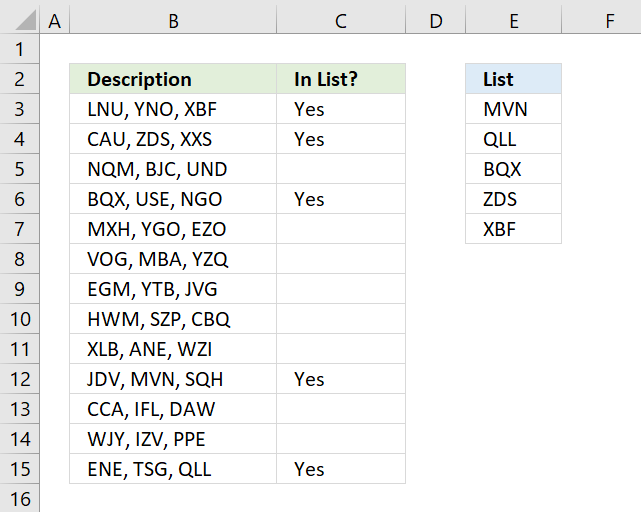
The image above shows an array formula in cell C3 that checks if cell B3 contains at least one of the values in List (E3:E7), it returns «Yes» if any of the values are found in column B and returns nothing if the cell contains none of the values.

For example, cell B3 contains XBF which is found in cell E7. Cell B4 contains text ZDS found in cell E6. Cell C5 contains no values in the list.

=IF(OR(COUNTIF(B3,»*»&$E$3:$E$7&»*»)), «Yes», «»)

You need to enter this formula as an array formula if you are not an Excel 365 subscriber. There is another formula below that doesn’t need to be entered as an array formula, however, it is slightly larger and more complicated.

Type formula in cell C3.
Press and hold CTRL + SHIFT simultaneously.
Press Enter once.
Release all keys.

Excel adds curly brackets to the formula automatically if you successfully entered the array formula. Don’t enter the curly brackets yourself.

1.1 Explaining formula in cell C3

Step 1 — Check if the cell contains any of the values in the list

The COUNTIF function lets you count cells based on a condition, however, it also allows you to count cells based on multiple conditions if you use a cell range instead of a cell.

COUNTIF(range, criteria)

The criteria argument utilizes a beginning and ending asterisk in order to match a text string and not the entire cell value, asterisks are one of two wildcard characters that you are allowed to use.

The ampersands concatenate the asterisks to cell range E3:E7.

COUNTIF(B3,»*»&$E$3:$E$7&»*»)

becomes

COUNTIF(«LNU, YNO, XBF», {«*MVN*»; «*QLL*»; «*BQX*»; «*ZDS*»; «*XBF*»})

and returns this array

{0; 0; 0; 0; 1}

which tells us that the last value in the list is found in cell B3.

Step 2 — Return TRUE if at least one value is 1

The OR function returns TRUE if at least one of the values in the array is TRUE, the numerical equivalent to TRUE is 1.

OR({0; 0; 0; 0; 1})

returns TRUE.

Step 3 — Return Yes or nothing

The IF function then returns «Yes» if the logical test evaluates to TRUE and nothing if the logical test returns FALSE.

IF(TRUE, «Yes», «»)

returns «Yes» in cell B3.

Regular formula

The following formula is quite similar to the formula above except that it is a regular formula and it has an additional INDEX function.

=IF(OR(INDEX(COUNTIF(B3,»*»&$E$3:$E$7&»*»),)), «Yes», «»)

2. Display matches if the cell contains text from a list

The image above demonstrates a formula that checks if a cell contains a value in the list and then returns that value. If multiple values match then all matching values in the list are displayed.

For example, cell B3 contains «ZDS, YNO, XBF» and cell range E3:E7 has two values that match, «ZDS» and «XBF».

Formula in cell C3:

=TEXTJOIN(«, «, TRUE, IF(COUNTIF(B3, «*»&$E$3:$E$7&»*»), $E$3:$E$7, «»))

The TEXTJOIN function is available for Office 2019 and Office 365 subscribers. You will get a #NAME error if your Excel version is missing this function. Office 2019 users may need to enter this formula as an array formula.

The next formula works with most Excel versions.

Array formula in cell C3:

=INDEX($E$3:$E$7, MATCH(1, COUNTIF(B3, «*»&$E$3:$E$7&»*»), 0))

However, it only returns the first match. There is another formula below that returns all matching values, check it out.

How to enter an array formula

2.1 Explaining formula in cell C3

Step 1 — Count cells containing text strings

The COUNTIF function lets you count cells based on a condition, we are going to use multiple conditions. I am going to use asterisks to make the COUNTIF function check for a partial match.

The asterisk is one of two wild card characters that you can use, it matches 0 (zero) to any number of any characters.

COUNTIF(B3, «*»&$E$3:$E$7&»*»)

becomes

COUNTIF(«ZDS, YNO, XBF», {«*MVN*»; «*QLL*»; «*BQX*»; «*ZDS*»; «*XBF*»})

and returns {1; 0; 0; 0; 1}.

This array contains as many values as there values in the list, the position of each value in the array matches the position of the value in the list. This means that we can tell from the array that the first value and the last value is found in cell B3.

Step 2 — Return the actual value

The IF function returns one value if the logical test is TRUE and another value if the logical test is FALSE.

IF(logical_test, [value_if_true], [value_if_false])

This allows us to create an array containing values that exists in cell B3.

IF(COUNTIF(B3, «*»&$E$3:$E$7&»*»), $E$3:$E$7, «»)

becomes

IF(COUNTIF(«ZDS, YNO, XBF», {«*MVN*»; «*QLL*»; «*BQX*»; «*ZDS*»; «*XBF*»}), {«*MVN*»; «*QLL*»; «*BQX*»; «*ZDS*»; «*XBF*»}, «»)

and returns {«»;»»;»»;»ZDS»;»XBF»}.

Step 3 — Concatenate values in array

The TEXTJOIN function allows you to combine text strings from multiple cell ranges and also use delimiting characters if you want.

TEXTJOIN(delimiter, ignore_empty, text1, [text2], …)

TEXTJOIN(«, «, TRUE, IF(COUNTIF(B3, «*»&$E$3:$E$7&»*»), $E$3:$E$7, «»))

becomes

TEXTJOIN(«, «, TRUE, {«»;»»;»»;»ZDS»;»XBF»})

and returns text strings ZDS, XBF.

3. Display matches if cell contains text from a list (Earlier Excel versions)

The image above demonstrates a formula that returns multiple matches if the cell contains values from a list. This array formula works with most Excel versions.

Array formula in cell C3:

=IFERROR(INDEX($G$3:$G$7, SMALL(IF(COUNTIF($B3, «*»&$G$3:$G$7&»*»), MATCH(ROW($G$3:$G$7), ROW($G$3:$G$7)), «»), COLUMNS($A$1:A1))), «»)

How to enter an array formula

Copy cell C3 and paste to cell range C3:E15.

3.1 Explaining formula in cell C3

Step 1 — Identify matching values in cell

The COUNTIF function lets you count cells based on a condition, we are going to use a cell range instead. This will return an array of values.

COUNTIF($B3, «*»&$G$3:$G$7&»*»)

becomes

COUNTIF(«ZDS, YNO, XBF», {«*MVN*»; «*QLL*»; «*BQX*»; «*ZDS*»; «*XBF*»})

and returns {0; 0; 0; 1; 1}.

Step 2 — Calculate relative positions of matching values

The IF function returns one value if the logical test is TRUE and another value if the logical test is FALSE.

IF(logical_test, [value_if_true], [value_if_false])

This allows us to create an array containing values representing row numbers.

IF(COUNTIF($B3, «*»&$G$3:$G$7&»*»), MATCH(ROW($G$3:$G$7), ROW($G$3:$G$7)), «»)

becomes

IF({0; 0; 0; 2; 1}, MATCH(ROW($G$3:$G$7), ROW($G$3:$G$7)), «»)

becomes

IF({0; 0; 0; 2; 1}, {1; 2; 3; 4; 5}, «»)

and returns {«»; «»; «»; 4; 5}.

Step 3 — Extract the k-th smallest number

I am going to use the SMALL function to be able to extract one value in each cell in the next step.

SMALL(array, k)

SMALL(IF(COUNTIF($B3, «*»&$G$3:$G$7&»*»), MATCH(ROW($G$3:$G$7), ROW($G$3:$G$7)), «»), COLUMNS($A$1:A1)))

becomes

SMALL({«»; «»; «»; 4; 5}, COLUMNS($A$1:A1)))

The COLUMNS function calculates the number of columns in a cell range, however, the cell reference in our formula grows when you copy the cell and paste to adjacent cells to the right.

SMALL({0; 0; 0; 4; 5}, COLUMNS($A$1:A1)))

becomes

SMALL({«»; «»; «»; 4; 5}, 1)

and returns 4.

Step 4 — Return value based on row number

The INDEX function returns a value from a cell range or array, you specify which value based on a row and column number. Both the [row_num] and [column_num] are optional.

INDEX(array, [row_num], [column_num])

INDEX($G$3:$G$7, SMALL(IF(COUNTIF($B3, «*»&$G$3:$G$7&»*»), MATCH(ROW($G$3:$G$7), ROW($G$3:$G$7)), «»), COLUMNS($A$1:A1)))

becomes

INDEX($G$3:$G$7, 4)

becomes

INDEX({«MVN»;»QLL»;»BQX»;»ZDS»;»XBF»}, 4)

and returns «ZDS» in cell C3.

Step 5 — Remove error values

The IFERROR function lets you catch most errors in Excel formulas except #SPILL! errors. Be careful when using the IFERROR function, it may make it much harder spotting formula errors.

IFERROR(value, value_if_error)

There are two arguments in the IFERROR function. The value argument is returned if it is not evaluating to an error. The value_if_error argument is returned if the value argument returns an error.

IFERROR(INDEX($G$3:$G$7, SMALL(IF(COUNTIF($B3, «*»&$G$3:$G$7&»*»), MATCH(ROW($G$3:$G$7), ROW($G$3:$G$7)), «»), COLUMNS($A$1:A1))), «»)

4. Filter delimited values not in the list (Excel 365)

The formula in cell C3 lists values in cell B3 that are not in the List specified in cell range E3:E7. The formula returns #CALC! error if all values are in the list, see cell C14 as an example.

Excel 365 dynamic array formula in cell C3:

=LET(z,TRIM(TEXTSPLIT(B3,,»,»)),TEXTJOIN(«, «,TRUE,FILTER(z,NOT(COUNTIF($E$3:$E$7,z)))))

4.1 Explaining formula

Step 1 — Split values with a delimiting character

The TEXTSPLIT function splits a string into an array based on delimiting values.

Function syntax: TEXTSPLIT(Input_Text, col_delimiter, [row_delimiter], [Ignore_Empty])

TEXTSPLIT(B3,,»,»)

becomes

TEXTSPLIT(«ZDS, VTO, XBF»,,»,»)

and returns

{«ZDS»; » VTO»; » XBF»}

Step 2 — Remove leading and trailing spaces

The TRIM function deletes all blanks or space characters except single blanks between words in a cell value.

Function syntax: TRIM(text)

TRIM(TEXTSPLIT(B3,,»,»))

becomes

TRIM({«ZDS»; » VTO»; » XBF»})

and returns

{«ZDS»; «VTO»; «XBF»}

Step 3 — Check if values are in list

The COUNTIF function calculates the number of cells that is equal to a condition.

Function syntax: COUNTIF(range, criteria)

COUNTIF($E$3:$E$7,TRIM(TEXTSPLIT(B3,,»,»)))

becomes

COUNTIF({«MVN»;»QLL»;»BQX»;»ZDS»;»XBF»},{«ZDS»; «VTO»; «XBF»})

and returns

{1; 0; 1}

These numbers indicate if a value is found in the list, zero means not in the list and 1 or higher means that the value is in the list at least once.

The number’s position corresponds to the position of the values. {1; 0; 1} — {«ZDS»; «VTO»; «XBF»} meaning «ZDS» and «XBF» are in the list and «VTO» not.

Step 4 — Not

The NOT function returns the boolean opposite to the given argument.

Function syntax: NOT(logical)

NOT(COUNTIF($E$3:$E$7,TRIM(TEXTSPLIT(B3,,»,»))))

becomes

NOT({1; 0; 1})

and returns

{FALSE; TRUE; FALSE}.

0 (zero) is equivalent to FALSE. The boolean opposite is TRUE.

Any other number than 0 (zero) is equivalent to TRUE. The boolean opposite is FALSE.

Step 5 — Filter

The FILTER function extracts values/rows based on a condition or criteria.

Function syntax: FILTER(array, include, [if_empty])

FILTER(TRIM(TEXTSPLIT(B3,,»,»)),NOT(COUNTIF($E$3:$E$7,TRIM(TEXTSPLIT(B3,,»,»)))))

becomes

FILTER({«ZDS»; «VTO»; «XBF»},{FALSE; TRUE; FALSE})

and returns

«VTO».

Step 6 — Join

The TEXTJOIN function combines text strings from multiple cell ranges.

Function syntax: TEXTJOIN(delimiter, ignore_empty, text1, [text2], …)

TEXTJOIN(«, «,TRUE,FILTER(TRIM(TEXTSPLIT(B3,,»,»)),NOT(COUNTIF($E$3:$E$7,TRIM(TEXTSPLIT(B3,,»,»))))))

becomes

TEXTJOIN(«, «,TRUE,{«VTO»})

and returns

«VTO».

Step 7 — Shorten the formula

The LET function lets you name intermediate calculation results which can shorten formulas considerably and improve performance.

Function syntax: LET(name1, name_value1, calculation_or_name2, [name_value2, calculation_or_name3…])

TEXTJOIN(«, «,TRUE,FILTER(TRIM(TEXTSPLIT(B3,,»,»)),NOT(COUNTIF($E$3:$E$7,TRIM(TEXTSPLIT(B3,,»,»))))))

z — TRIM(TEXTSPLIT(B3,,»,»))

LET(z,TRIM(TEXTSPLIT(B3,,»,»)),TEXTJOIN(«, «,TRUE,FILTER(z,NOT(COUNTIF($E$3:$E$7,z)))))

Источник

The logical IF statement in Excel is used for the recording of certain conditions. It compares the number and / or text, function, etc. of the formula when the values correspond to the set parameters, and then there is one record, when do not respond — another.

Logic functions — it is a very simple and effective tool that is often used in practice. Let us consider it in details by examples.

The syntax of the function «IF» with one condition

The operation syntax in Excel is the structure of the functions necessary for its operation data.

=IF(boolean;value_if_TRUE;value_if_FALSE)

Let us consider the function syntax:

Boolean – what the operator checks (text or numeric data cell).
Value_if_TRUE – what will appear in the cell when the text or numbers correspond to a predetermined condition (true).
Value_if_FALSE – what appears in the box when the text or the number does not meet the predetermined condition (false).

Example:

Logical IF functions.

The operator checks the A1 cell and compares it to 20. This is a «Boolean». When the contents of the column is more than 20, there is a true legend «greater 20». In the other case it’s «less or equal 20».

Attention! The words in the formula need to be quoted. For Excel to understand that you want to display text values.

Here is one more example. To gain admission to the exam, a group of students must successfully pass a test. The results are listed in a table with columns: a list of students, a credit, an exam.

list.

The statement IF should check not the digital data type but the text. Therefore, we prescribed in the formula В2= «done» We take the quotes for the program to recognize the text correctly.

The function IF in Excel with multiple conditions

Usually one condition for the logic function is not enough. If you need to consider several options for decision-making, spread operators’ IF into each other. Thus, we get several functions IF in Excel.

The syntax is as follows:

Here the operator checks the two parameters. If the first condition is true, the formula returns the first argument is the truth. False — the operator checks the second condition.

Examples of a few conditions of the function IF in Excel:

It’s a table for the analysis of the progress. The student received 5 points:

А – excellent;
В – above average or superior work;
C – satisfactory;
D – a passing grade;
E – completely unsatisfactory.

IF statement checks two conditions: the equality of value in the cells.

In this example, we have added a third condition, which implies the presence of another report card and «twos». The principle of the operator is the same.

Enhanced functionality with the help of the operators «AND» and «OR»

When you need to check out a few of the true conditions you use the function И. The point is: IF A = 1 AND A = 2 THEN meaning в ELSE meaning с.

OR function checks the condition 1 or condition 2. As soon as at least one condition is true, the result is true. The point is: IF A = 1 OR A = 2 THEN value B ELSE value C.

Functions AND & OR can check up to 30 conditions.

An example of using the operator AND:

It’s the example of using the logical operator OR.

How to compare data in two tables

Users often need to compare the two spreadsheets in an Excel to match. Examples of the «life»: compare the prices of goods in different bringing, to compare balances (accounting reports) in a few months, the progress of pupils (students) of different classes, in different quarters, etc.

To compare the two tables in Excel, you can use the COUNTIFS statement. Consider the order of application functions.

For example, consider the two tables with the specifications of various food processors. We planned allocation of color differences. This problem in Excel solves the conditional formatting.

Baseline data (tables, which will work with):

tables.

Select the first table. Conditional Formatting — create a rule — use a formula to determine the formatted cells:

In the formula bar write: = COUNTIFS (comparable range; first cell of first table)=0. Comparing range is in the second table.

To drive the formula into the range, just select it first cell and the last. «= 0» means the search for the exact command (not approximate) values.

Choose the format and establish what changes in the cell formula in compliance. It’s better to do a color fill.

Select the second table. Conditional Formatting — create a rule — use the formula. Use the same operator (COUNTIFS). For the second table formula:

Download all examples in Excel

Now it is easy to compare the characteristics of the data in the table.

Источник

Check If Value In Range Using COUNTIF Function

Excel Find Value is in Range Example

How to check if a value is in Range with Wild Card Operators

Find if a Value is in a List Using MATCH Function

Simple IF examples

Common problems

Need more help?

See Also

Need more help?

Dependent dropdown lists

What’s on this page

1. Check if the cell contains any value in the list

1.1 Explaining formula in cell C3

Step 1 — Check if the cell contains any of the values in the list

Step 2 — Return TRUE if at least one value is 1

Step 3 — Return Yes or nothing

Regular formula

2. Display matches if the cell contains text from a list

2.1 Explaining formula in cell C3

Step 1 — Count cells containing text strings

Step 2 — Return the actual value

Step 3 — Concatenate values in array

3. Display matches if cell contains text from a list (Earlier Excel versions)

3.1 Explaining formula in cell C3

Step 1 — Identify matching values in cell

Step 2 — Calculate relative positions of matching values

Step 3 — Extract the k-th smallest number

Step 4 — Return value based on row number

Step 5 — Remove error values

4. Filter delimited values not in the list (Excel 365)

4.1 Explaining formula

Step 1 — Split values with a delimiting character

Step 2 — Remove leading and trailing spaces

Step 3 — Check if values are in list

Step 4 — Not

Step 5 — Filter

Step 6 — Join

Step 7 — Shorten the formula

The syntax of the function «IF» with one condition

The function IF in Excel with multiple conditions

Enhanced functionality with the help of the operators «AND» and «OR»

How to compare data in two tables