
Excel for Microsoft 365 Excel 2021 Excel 2019 Excel 2016 Excel 2013 Excel 2010 Excel 2007 More…Less
Let’s say you want to ensure that a column contains text, not numbers. Or, perhapsyou want to find all orders that correspond to a specific salesperson. If you have no concern for upper- or lowercase text, there are several ways to check if a cell contains text.
You can also use a filter to find text. For more information, see Filter data.
Find cells that contain text
Follow these steps to locate cells containing specific text:
-
Select the range of cells that you want to search.
To search the entire worksheet, click any cell.
-
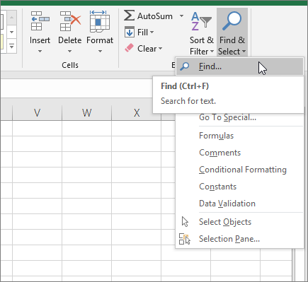
On the Home tab, in the Editing group, click Find & Select, and then click Find.

-
In the Find what box, enter the text—or numbers—that you need to find. Or, choose a recent search from the Find what drop-down box.
Note: You can use wildcard characters in your search criteria.
-
To specify a format for your search, click Format and make your selections in the Find Format popup window.
-
Click Options to further define your search. For example, you can search for all of the cells that contain the same kind of data, such as formulas.
In the Within box, you can select Sheet or Workbook to search a worksheet or an entire workbook.
-
Click Find All or Find Next.
Find All lists every occurrence of the item that you need to find, and allows you to make a cell active by selecting a specific occurrence. You can sort the results of a Find All search by clicking a header.
Note: To cancel a search in progress, press ESC.
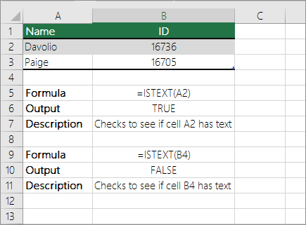
Check if a cell has any text in it
To do this task, use the ISTEXT function.
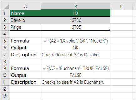
Check if a cell matches specific text
Use the IF function to return results for the condition that you specify.
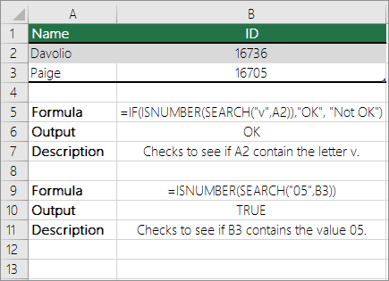
Check if part of a cell matches specific text
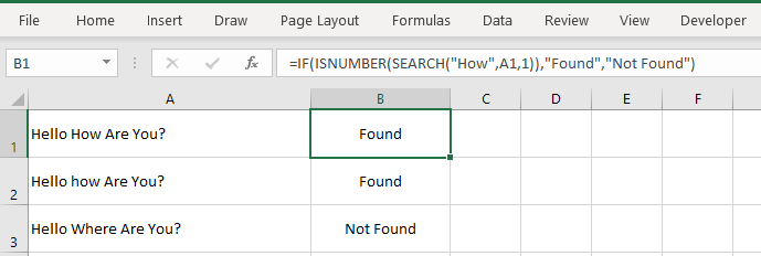
To do this task, use the IF, SEARCH, and ISNUMBER functions.
Note: The SEARCH function is case-insensitive.
Need more help?
One limitation of the IF function is that it does not support wildcards like «?» and «*». This means you can’t use IF by itself to test for text that may appear anywhere in a cell.
One solution is a formula that uses the IF function together with the SEARCH and ISNUMBER functions. In the example shown, we have a list of email addresses, and we want to extract those that contain «abc». In C5, the formula were using is this:
=IF(ISNUMBER(SEARCH("abc",B5)),B5,"")
If «abc» is found anywhere in cell B5, IF will return that value. If not, IF will return an empty string («»). In this formula, the logical test is this bit:
ISNUMBER(SEARCH("abc",B5))
This snippet will return TRUE if the the value in B5 contains «abc» and false if not. The logic of ISNUMBER + SEARCH is explained in detail here.
To copy cell the value in B5 when it contains «abc», we provide B5 again for the «value if true» argument. If FALSE, we supply an empty string («») which will display as a blank cell on the worksheet.
Excel has a number of formulas that help you use your data in useful ways. For example, you can get an output based on whether or not a cell meets certain specifications. Right now, we’ll focus on a function called “if cell contains, then”. Let’s look at an example.
Jump To Specific Section:
- Explanation: If Cell Contains
- If cell contains any value, then return a value
- If cell contains text/number, then return a value
- If cell contains specific text, then return a value
- If cell contains specific text, then return a value (case-sensitive)
- If cell does not contain specific text, then return a value
- If cell contains one of many text strings, then return a value
- If cell contains several of many text strings, then return a value
Excel Formula: If cell contains
Generic formula
=IF(ISNUMBER(SEARCH("abc",A1)),A1,"")
Summary
To test for cells that contain certain text, you can use a formula that uses the IF function together with the SEARCH and ISNUMBER functions. In the example shown, the formula in C5 is:
=IF(ISNUMBER(SEARCH("abc",B5)),B5,"")
If you want to check whether or not the A1 cell contains the text “Example”, you can run a formula that will output “Yes” or “No” in the B1 cell. There are a number of different ways you can put these formulas to use. At the time of writing, Excel is able to return the following variations:
- If cell contains any value
- If cell contains text
- If cell contains number
- If cell contains specific text
- If cell contains certain text string
- If cell contains one of many text strings
- If cell contains several strings
Using these scenarios, you’re able to check if a cell contains text, value, and more.
Explanation: If Cell Contains
One limitation of the IF function is that it does not support Excel wildcards like «?» and «*». This simply means you can’t use IF by itself to test for text that may appear anywhere in a cell.
One solution is a formula that uses the IF function together with the SEARCH and ISNUMBER functions. For example, if you have a list of email addresses, and want to extract those that contain «ABC», the formula to use is this:
=IF(ISNUMBER(SEARCH("abc",B5)),B5,""). Assuming cells run to B5
If «abc» is found anywhere in a cell B5, IF will return that value. If not, IF will return an empty string («»). This formula’s logical test is this bit:
ISNUMBER(SEARCH("abc",B5))
Read article: Excel efficiency: 11 Excel Formulas To Increase Your Productivity
Using “if cell contains” formulas in Excel
The guides below were written using the latest Microsoft Excel 2019 for Windows 10. Some steps may vary if you’re using a different version or platform. Contact our experts if you need any further assistance.
1. If cell contains any value, then return a value
This scenario allows you to return values based on whether or not a cell contains any value at all. For example, we’ll be checking whether or not the A1 cell is blank or not, and then return a value depending on the result.
- Select the output cell, and use the following formula: =IF(cell<>»», value_to_return, «»).
- For our example, the cell we want to check is A2, and the return value will be No. In this scenario, you’d change the formula to =IF(A2<>»», «No», «»).
- Since the A2 cell isn’t blank, the formula will return “No” in the output cell. If the cell you’re checking is blank, the output cell will also remain blank.
2. If cell contains text/number, then return a value
With the formula below, you can return a specific value if the target cell contains any text or number. The formula will ignore the opposite data types.
Check for text
- To check if a cell contains text, select the output cell, and use the following formula: =IF(ISTEXT(cell), value_to_return, «»).
- For our example, the cell we want to check is A2, and the return value will be Yes. In this scenario, you’d change the formula to =IF(ISTEXT(A2), «Yes», «»).

- Because the A2 cell does contain text and not a number or date, the formula will return “Yes” into the output cell.
Check for a number or date
- To check if a cell contains a number or date, select the output cell, and use the following formula: =IF(ISNUMBER(cell), value_to_return, «»).
- For our example, the cell we want to check is D2, and the return value will be Yes. In this scenario, you’d change the formula to =IF(ISNUMBER(D2), «Yes», «»).

- Because the D2 cell does contain a number and not text, the formula will return “Yes” into the output cell.
3. If cell contains specific text, then return a value
To find a cell that contains specific text, use the formula below.
- Select the output cell, and use the following formula: =IF(cell=»text», value_to_return, «»).
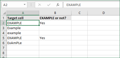
- For our example, the cell we want to check is A2, the text we’re looking for is “example”, and the return value will be Yes. In this scenario, you’d change the formula to =IF(A2=»example», «Yes», «»).

- Because the A2 cell does consist of the text “example”, the formula will return “Yes” into the output cell.
4. If cell contains specific text, then return a value (case-sensitive)
To find a cell that contains specific text, use the formula below. This version is case-sensitive, meaning that only cells with an exact match will return the specified value.
- Select the output cell, and use the following formula: =IF(EXACT(cell,»case_sensitive_text»), «value_to_return», «»).
- For our example, the cell we want to check is A2, the text we’re looking for is “EXAMPLE”, and the return value will be Yes. In this scenario, you’d change the formula to =IF(EXACT(A2,»EXAMPLE»), «Yes», «»).
- Because the A2 cell does consist of the text “EXAMPLE” with the matching case, the formula will return “Yes” into the output cell.
5. If cell does not contain specific text, then return a value
The opposite version of the previous section. If you want to find cells that don’t contain a specific text, use this formula.
- Select the output cell, and use the following formula: =IF(cell=»text», «», «value_to_return»).
- For our example, the cell we want to check is A2, the text we’re looking for is “example”, and the return value will be No. In this scenario, you’d change the formula to =IF(A2=»example», «», «No»).
- Because the A2 cell does consist of the text “example”, the formula will return a blank cell. On the other hand, other cells return “No” into the output cell.
6. If cell contains one of many text strings, then return a value
This formula should be used if you’re looking to identify cells that contain at least one of many words you’re searching for.
- Select the output cell, and use the following formula: =IF(OR(ISNUMBER(SEARCH(«string1», cell)), ISNUMBER(SEARCH(«string2», cell))), value_to_return, «»).
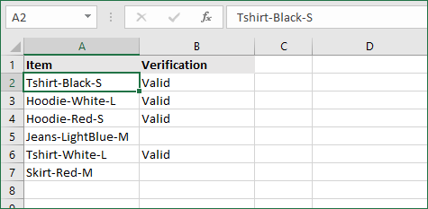
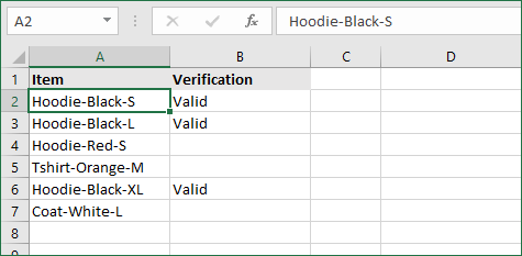
- For our example, the cell we want to check is A2. We’re looking for either “tshirt” or “hoodie”, and the return value will be Valid. In this scenario, you’d change the formula to =IF(OR(ISNUMBER(SEARCH(«tshirt»,A2)),ISNUMBER(SEARCH(«hoodie»,A2))),»Valid «,»»).
- Because the A2 cell does contain one of the text values we searched for, the formula will return “Valid” into the output cell.
To extend the formula to more search terms, simply modify it by adding more strings using ISNUMBER(SEARCH(«string», cell)).
7. If cell contains several of many text strings, then return a value
This formula should be used if you’re looking to identify cells that contain several of the many words you’re searching for. For example, if you’re searching for two terms, the cell needs to contain both of them in order to be validated.
- Select the output cell, and use the following formula: =IF(AND(ISNUMBER(SEARCH(«string1»,cell)), ISNUMBER(SEARCH(«string2″,cell))), value_to_return,»»).
- For our example, the cell we want to check is A2. We’re looking for “hoodie” and “black”, and the return value will be Valid. In this scenario, you’d change the formula to =IF(AND(ISNUMBER(SEARCH(«hoodie»,A2)),ISNUMBER(SEARCH(«black»,A2))),»Valid «,»»).
- Because the A2 cell does contain both of the text values we searched for, the formula will return “Valid” to the output cell.
Final thoughts
We hope this article was useful to you in learning how to use “if cell contains” formulas in Microsoft Excel. Now, you can check if any cells contain values, text, numbers, and more. This allows you to navigate, manipulate and analyze your data efficiently.
We’re glad you’re read the article up to here  Thank you
You may also like
» How to use NPER Function in Excel
» How to Separate First and Last Name in Excel
» How to Calculate Break-Even Analysis in Excel
![]()
Excel If Cell Contains Text

Excel If Cell Contains Text Then Formula helps you to return the output when a cell have any text or a specific text. You can check if a cell contains a some string or text and produce something in other cell. For Example you can check if a cell A1 contains text ‘example text’ and print Yes or No in Cell B1. Following are the example Formulas to check if Cell contains text then return some thing in a Cell.
If Cell Contains Text
Here are the Excel formulas to check if Cell contains specific text then return something. This will return if there is any string or any text in given Cell. We can use this simple approach to check if a cell contains text, specific text, string, any text using Excel If formula. We can use equals to operator(=) to compare the strings .
If Cell Contains Text Then TRUE
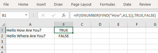
Following is the Excel formula to return True if a Cell contains Specif Text. You can check a cell if there is given string in the Cell and return True or False.
The formula will return true if it found the match, returns False of no match found.
If Cell Contains Partial Text
We can return Text If Cell Contains Partial Text. We use formula or VBA to Check Partial Text in a Cell.
Find for Case Sensitive Match:
We can check if a Cell Contains Partial Text then return something using Excel Formula. Following is a simple example to find the partial text in a given Cell. We can use if your want to make the criteria case sensitive.
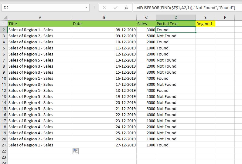
- Here, Find Function returns the finding position of the given string
- Use Find function is Case Sensitive
- IsError Function check if Find Function returns Error, that means, string not found
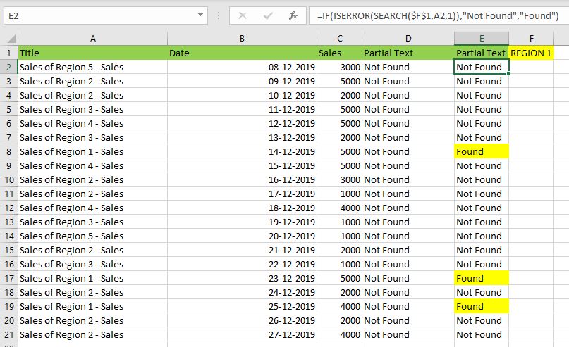
Search for Not Case Sensitive Match:
We can use Search function to check if Cell Contains Partial Text. Search function useful if you want to make the checking criteria Not Case Sensitive.
If Range of Cells Contains Text
We can check for the strings in a range of cells. Here is the formula to find If Range of Cells Contains Text. We can use Count If Formula to check the excel if range of cells contains specific text and return Text.
- CountIf function counts the number of cells with given criteria
- We can use If function to return the required Text
- Formula displays the Text ‘Range Contains Text” if match found
- Returns “Text Not Found in the Given Range” if match not found in the specified range
If Cells Contains Text From List
Below formulas returns text If Cells Contains Text from given List. You can use based on your requirement.
VlookUp to Check If Cell Contains Text from a List:
We can use VlookUp function to match the text in the Given list of Cells. And return the corresponding values.
- Check if a List Contains Text:
=IF(ISERR(VLOOKUP(F1,A1:B21,2,FALSE)),”False:Not Contains”,”True: Text Found”) - Check if a List Contains Text and Return Corresponding Value:
=VLOOKUP(F1,A1:B21,2,FALSE) - Check if a List Contains Partial Text and Return its Value:
=VLOOKUP(“*”&F1&”*”,A1:B21,2,FALSE)
If Cell Contains Text Then Return a Value
We can return some value if cell contains some string. Here is the the the Excel formula to return a value if a Cell contains Text. You can check a cell if there is given string in the Cell and return some string or value in another column.
The formula will return true if it found the match, returns False of no match found. can
Excel if cell contains word then assign value
You can replace any word in the following formula to check if cell contains word then assign value.
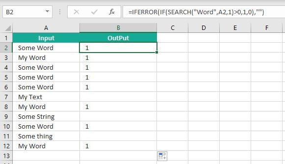
Search function will check for a given word in the required cell and return it’s position. We can use If function to check if the value is greater than 0 and assign a given value (example: 1) in the cell. search function returns #Value if there is no match found in the cell, we can handle this using IFERROR function.
Count If Cell Contains Text
We can check If Cell Contains Text Then COUNT. Here is the Excel formula to Count if a Cell contains Text. You can count the number of cells containing specific text.
The formula will Sum the values in Column B if the cells of Column A contains the given text.
Count If Cell Contains Partial Text
We can count the cells based on partial match criteria. The following Excel formula Counts if a Cell contains Partial Text.
- We can use the CountIf Function to Count the Cells if they contains given String
- Wild-card operators helps to make the CountIf to check for the Partial String
- Put Your Text between two asterisk symbols (*YourText*) to make the criteria to find any where in the given Cell
- Add Asterisk symbol at end of your text (YourText*) to make the criteria to find your text beginning of given Cell
- Place Asterisk symbol at beginning of your text (*YourText) to make the criteria to find your text end of given Cell
If Cell contains text from list then return value
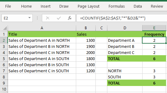
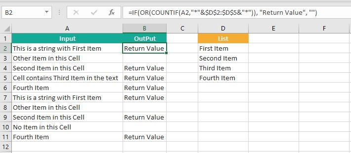
Here is the Excel Formula to check if cell contains text from list then return value. We can use COUNTIF and OR function to check the array of values in a Cell and return the given Value. Here is the formula to check the list in range D2:D5 and check in Cell A2 and return value in B2.
If Cell Contains Text Then SUM
Following is the Excel formula to Sum if a Cell contains Text. You can total the cell values if there is given string in the Cell. Here is the example to sum the column B values based on the values in another Column.
The formula will Sum the values in Column B if the cells of Column A contains the given text.

Sum If Cell Contains Partial Text
Use SumIfs function to Sum the cells based on partial match criteria. The following Excel formula Sums the Values if a Cell contains Partial Text.
- SUMIFS Function will Sum the Given Sum Range
- We can specify the Criteria Range, and wild-card expression to check for the Partial text
- Put Your Text between two asterisk symbols (*YourText*) to Sum the Cells if the criteria to find any where in the given Cell
- Add Asterisk symbol at end of your text (YourText*) to Sum the Cells if the criteria to find your text beginning of given Cell
- Place Asterisk symbol at beginning of your text (*YourText) to Sum the Cells if criteria to find your text end of given Cell
VBA to check if Cell Contains Text
Here is the VBA function to find If Cells Contains Text using Excel VBA Macros.
If Cell Contains Partial Text VBA
We can use VBA to check if Cell Contains Text and Return Value. Here is the simple VBA code match the partial text. Excel VBA if Cell contains partial text macros helps you to use in your procedures and functions.
MsgBox CheckIfCellContainsPartialText(Cells(2, 1), “Region 1”)
End Sub
Function CheckIfCellContainsPartialText(ByVal cell As Range, ByVal strText As String) As Boolean
If InStr(1, cell.Value, strText) > 0 Then CheckIfCellContainsPartialText = True
End Function
- CheckIfCellContainsPartialText VBA Function returns true if Cell Contains Partial Text
- inStr Function will return the Match Position in the given string
If Cell Contains Text Then VBA MsgBox
Here is the simple VBA code to display message box if cell contains text. We can use inStr Function to search for the given string. And show the required message to the user.
If InStr(1, Cells(2, 1), “Region 3”) > 0 Then blnMatch = True
If blnMatch = True Then MsgBox “Cell Contains Text”
End Sub
- inStr Function will return the Match Position in the given string
- blnMatch is the Boolean variable becomes True when match string
- You can display the message to the user if a Range Contains Text
Which function returns true if cell a1 contains text?
You can use the Excel If function and Find function to return TRUE if Cell A1 Contains Text. Here is the formula to return True.
Which function returns true if cell a1 contains text value?
You can use the Excel If function with Find function to return TRUE if a Cell A1 Contains Text Value. Below is the formula to return True based on the text value.
Share This Story, Choose Your Platform!
7 Comments
-
Meghana
December 27, 2019 at 1:42 pm — ReplyHi Sir,Thank you for the great explanation, covers everything and helps use create formulas if cell contains text values.
Many thanks! Meghana!!
-
Max
December 27, 2019 at 4:44 pm — ReplyPerfect! Very Simple and Clear explanation. Thanks!!
-
Mike Song
August 29, 2022 at 2:45 pm — ReplyI tried this exact formula and it did not work.
-
Theresa A Harding
October 18, 2022 at 9:51 pm — Reply -
Marko
November 3, 2022 at 9:21 pm — ReplyHi
Is possible to sum all WA11?
(A1) WA11 4
(A2) AdBlue 1, WA11 223
(A3) AdBlue 3, WA11 32, shift 4
… and everything is in one column.
Thanks you very much for your help.
Sincerely Marko
-
Mike
December 9, 2022 at 9:59 pm — ReplyThank you for the help. The formula =OR(COUNTIF(M40,”*”&Vendors&”*”)) will give “TRUE” when some part of M40 contains a vendor from “Vendors” list. But how do I get Excel to tell which vendor it found in the M40 cell?
-
PNRao
December 18, 2022 at 6:05 am — ReplyPlease describe your question more elaborately.
Thanks!
-
© Copyright 2012 – 2020 | Excelx.com | All Rights Reserved
Page load link
Содержание
- Check if a cell contains text (case-insensitive)
- Find cells that contain text
- Check if a cell has any text in it
- Check if a cell matches specific text
- Check if part of a cell matches specific text
- How To Use “If Cell Contains” Formulas in Excel
- Excel Formula: If cell contains
- Explanation: If Cell Contains
- Using “if cell contains” formulas in Excel
- 1. If cell contains any value, then return a value
- 2. If cell contains text/number, then return a value
- Check for text
- Check for a number or date
- 3. If cell contains specific text, then return a value
- 4. If cell contains specific text, then return a value (case-sensitive)
- 5. If cell does not contain specific text, then return a value
- 6. If cell contains one of many text strings, then return a value
- 7. If cell contains several of many text strings, then return a value
- Final thoughts
- Before you go
- Excel: If cell contains then count, sum, highlight, copy or delete
- Excel ‘Count if cell contains’ formula examples
- Count if cell contains any text
- Count if cell contains specific text
- Count if cell contains text (partial match)
- Count if cell contains multiple substrings (AND logic)
- Count if cell contains number
- Sum if cell contains text
- Perform different calculations based on cell value
- Excel conditional formatting if cell contains specific text
- Case-insensitive:
- Case-sensitive:
- Excel conditional formatting formula: if cell contains text (multiple conditions)
- If cell contains certain text, remove entire row
- If cell contains, select or copy entire rows
- Practice workbook
- You may also be interested in
Check if a cell contains text (case-insensitive)
Let’s say you want to ensure that a column contains text, not numbers. Or, perhapsyou want to find all orders that correspond to a specific salesperson. If you have no concern for upper- or lowercase text, there are several ways to check if a cell contains text.
You can also use a filter to find text. For more information, see Filter data.
Find cells that contain text
Follow these steps to locate cells containing specific text:
Select the range of cells that you want to search.
To search the entire worksheet, click any cell.
On the Home tab, in the Editing group, click Find & Select, and then click Find.
In the Find what box, enter the text—or numbers—that you need to find. Or, choose a recent search from the Find what drop-down box.
Note: You can use wildcard characters in your search criteria.
To specify a format for your search, click Format and make your selections in the Find Format popup window.
Click Options to further define your search. For example, you can search for all of the cells that contain the same kind of data, such as formulas.
In the Within box, you can select Sheet or Workbook to search a worksheet or an entire workbook.
Click Find All or Find Next.
Find All lists every occurrence of the item that you need to find, and allows you to make a cell active by selecting a specific occurrence. You can sort the results of a Find All search by clicking a header.
Note: To cancel a search in progress, press ESC.
Check if a cell has any text in it
To do this task, use the ISTEXT function.
Check if a cell matches specific text
Use the IF function to return results for the condition that you specify.
Check if part of a cell matches specific text
To do this task, use the IF, SEARCH, and ISNUMBER functions.
Note: The SEARCH function is case-insensitive.
Источник
How To Use “If Cell Contains” Formulas in Excel
Excel has a number of formulas that help you use your data in useful ways. For example, you can get an output based on whether or not a cell meets certain specifications. Right now, we’ll focus on a function called “if cell contains, then”. Let’s look at an example.

Excel Formula: If cell contains
To test for cells that contain certain text, you can use a formula that uses the IF function together with the SEARCH and ISNUMBER functions. In the example shown, the formula in C5 is:
If you want to check whether or not the A1 cell contains the text “Example”, you can run a formula that will output “Yes” or “No” in the B1 cell. There are a number of different ways you can put these formulas to use. At the time of writing, Excel is able to return the following variations:
- If cell contains any value
- If cell contains text
- If cell contains number
- If cell contains specific text
- If cell contains certain text string
- If cell contains one of many text strings
- If cell contains several strings
Using these scenarios, you’re able to check if a cell contains text, value, and more.
Explanation: If Cell Contains
One limitation of the IF function is that it does not support Excel wildcards like «?» and «*». This simply means you can’t use IF by itself to test for text that may appear anywhere in a cell.
One solution is a formula that uses the IF function together with the SEARCH and ISNUMBER functions. For example, if you have a list of email addresses, and want to extract those that contain «ABC», the formula to use is this:
If «abc» is found anywhere in a cell B5, IF will return that value. If not, IF will return an empty string («»). This formula’s logical test is this bit:
Using “if cell contains” formulas in Excel
The guides below were written using the latest Microsoft Excel 2019 for Windows 10 . Some steps may vary if you’re using a different version or platform. Contact our experts if you need any further assistance.
1. If cell contains any value, then return a value
This scenario allows you to return values based on whether or not a cell contains any value at all. For example, we’ll be checking whether or not the A1 cell is blank or not, and then return a value depending on the result.
- Select the output cell, and use the following formula: =IF(cell<>«», value_to_return, «») .
- For our example, the cell we want to check is A2 , and the return value will be No . In this scenario, you’d change the formula to =IF(A2<>«», «No», «») .
2. If cell contains text/number, then return a value
With the formula below, you can return a specific value if the target cell contains any text or number. The formula will ignore the opposite data types.
Check for text
- To check if a cell contains text, select the output cell, and use the following formula: =IF(ISTEXT(cell), value_to_return, «») .
- For our example, the cell we want to check is A2 , and the return value will be Yes . In this scenario, you’d change the formula to =IF(ISTEXT(A2), «Yes», «») .
- Because the A2 cell does contain text and not a number or date, the formula will return “ Yes ” into the output cell.
Check for a number or date
- To check if a cell contains a number or date, select the output cell, and use the following formula: =IF(ISNUMBER(cell), value_to_return, «») .
- For our example, the cell we want to check is D2 , and the return value will be Yes . In this scenario, you’d change the formula to =IF(ISNUMBER(D2), «Yes», «») .
- Because the D2 cell does contain a number and not text, the formula will return “ Yes ” into the output cell.
3. If cell contains specific text, then return a value
To find a cell that contains specific text, use the formula below.
- Select the output cell, and use the following formula: =IF(cell=»text», value_to_return, «») .
- For our example, the cell we want to check is A2 , the text we’re looking for is “ example ”, and the return value will be Yes . In this scenario, you’d change the formula to =IF(A2=»example», «Yes», «») .
- Because the A2 cell does consist of the text “ example ”, the formula will return “ Yes ” into the output cell.
4. If cell contains specific text, then return a value (case-sensitive)
To find a cell that contains specific text, use the formula below. This version is case-sensitive, meaning that only cells with an exact match will return the specified value.
- Select the output cell, and use the following formula: =IF(EXACT(cell,»case_sensitive_text»), «value_to_return», «») .
- For our example, the cell we want to check is A2 , the text we’re looking for is “ EXAMPLE ”, and the return value will be Yes . In this scenario, you’d change the formula to =IF(EXACT(A2,»EXAMPLE»), «Yes», «») .
- Because the A2 cell does consist of the text “ EXAMPLE ” with the matching case, the formula will return “ Yes ” into the output cell.
5. If cell does not contain specific text, then return a value
The opposite version of the previous section. If you want to find cells that don’t contain a specific text, use this formula.
- Select the output cell, and use the following formula: =IF(cell=»text», «», «value_to_return») .
- For our example, the cell we want to check is A2 , the text we’re looking for is “ example ”, and the return value will be No . In this scenario, you’d change the formula to =IF(A2=»example», «», «No») .
- Because the A2 cell does consist of the text “ example ”, the formula will return a blank cell. On the other hand, other cells return “ No ” into the output cell.
6. If cell contains one of many text strings, then return a value
This formula should be used if you’re looking to identify cells that contain at least one of many words you’re searching for.
- Select the output cell, and use the following formula: =IF(OR(ISNUMBER(SEARCH(«string1», cell)), ISNUMBER(SEARCH(«string2», cell))), value_to_return, «») .
- For our example, the cell we want to check is A2 . We’re looking for either “ tshirt ” or “ hoodie ”, and the return value will be Valid . In this scenario, you’d change the formula to =IF(OR(ISNUMBER(SEARCH(«tshirt»,A2)),ISNUMBER(SEARCH(«hoodie»,A2))),»Valid «,»») .
- Because the A2 cell does contain one of the text values we searched for, the formula will return “ Valid ” into the output cell.
To extend the formula to more search terms, simply modify it by adding more strings using ISNUMBER(SEARCH(«string», cell)) .
7. If cell contains several of many text strings, then return a value
This formula should be used if you’re looking to identify cells that contain several of the many words you’re searching for. For example, if you’re searching for two terms, the cell needs to contain both of them in order to be validated.
- Select the output cell, and use the following formula: =IF(AND(ISNUMBER(SEARCH(«string1»,cell)), ISNUMBER(SEARCH(«string2″,cell))), value_to_return,»») .
- For our example, the cell we want to check is A2 . We’re looking for “ hoodie ” and “ black ”, and the return value will be Valid . In this scenario, you’d change the formula to =IF(AND(ISNUMBER(SEARCH(«hoodie»,A2)),ISNUMBER(SEARCH(«black»,A2))),»Valid «,»») .
- Because the A2 cell does contain both of the text values we searched for, the formula will return “ Valid ” to the output cell.
Final thoughts
We hope this article was useful to you in learning how to use “if cell contains” formulas in Microsoft Excel. Now, you can check if any cells contain values, text, numbers, and more. This allows you to navigate, manipulate and analyze your data efficiently.
We’re glad you’re read the article up to here 🙂 Thank you 🙂
Please share it on your socials. Someone else will benefit.
Before you go
If you need any further help with Excel, don’t hesitate to reach out to our customer service team, which is available 24/7 to assist you. Return to us for more informative articles all related to productivity and modern-day technology!
Would you like to receive promotions, deals, and discounts to get our products for the best price? Don’t forget to subscribe to our newsletter by entering your email address below! Receive the latest technology news in your inbox and be the first to read our tips to become more productive.
Источник
Excel: If cell contains then count, sum, highlight, copy or delete
 by Svetlana Cheusheva, updated on March 17, 2023
In our previous tutorial, we were looking at Excel If contains formulas that return some value to another column if a target cell contains a given value. Aside from that, what else can you do if a cell contains specific text or number? A variety of things such as counting or summing cells, highlighting, removing or copying entire rows, and more.
Excel ‘Count if cell contains’ formula examples
In Microsoft Excel, there are two functions to count cells based on their values, COUNTIF and COUNTIFS. These functions cover most, though not all, scenarios. The below examples will teach you how to choose an appropriate Count if cell contains formula for your particular task.
Count if cell contains any text
In situations when you want to count cells containing any text, use the asterisk wildcard character as the criteria in your COUNTIF formula:
Or, use the SUMPRODUCT function in combination with ISTEXT:
In the second formula, the ISTEXT function evaluates each cell in the specified range and returns an array of TRUE (text) and FALSE (not text) values; the double unary operator (—) coerces TRUE and FALSE into 1’s and 0’s; and SUMPRODUCT adds up the numbers.
As shown in the screenshot below, both formulas yield the same result:
=SUMPRODUCT(—(ISTEXT(A2:A10))) 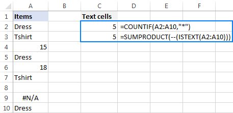
You may also want to look at how to count non-empty cells in Excel.
Count if cell contains specific text
To count cells that contain specific text, use a simple COUNTIF formula like shown below, where range is the cells to check and text is the text string to search for or a reference to the cell containing the text string.
For example, to count cells in the range A2:A10 that contain the word «dress», use this formula:
Or the one shown in the screenshot: 
Count if cell contains text (partial match)
To count cells that contain a certain substring, use the COUNTIF function with the asterisk wildcard character (*).
For example, to count how many cells in column A contain «dress» as part of their contents, use this formula:
Or, type the desired text in some cell and concatenate that cell with the wildcard characters:
=COUNTIF(A2:A10,»*»&D1&»*») 
Count if cell contains multiple substrings (AND logic)
To count cells with multiple conditions, use the COUNTIFS function. Excel COUNTIFS can handle up to 127 range/criteria pairs, and only cells that meet all of the specified conditions will be counted.
For example, to find out how many cells in column A contain «dress» AND «blue», use one of the following formulas:
=COUNTIFS(A2:A10,»*»&D1&»*», A2:A10,»*»&D2&»*») 
Count if cell contains number
The formula to count cells with numbers is the simplest formula one could imagine:
Please keep in mind that the COUNT function in Excel counts cells containing any numeric value including numbers, dates and times, because in terms of Excel the last two are also numbers.
In our case, the formula goes as follows:
To count cells that DO NOT contain numbers, use the SUMPRODUCT function together with ISNUMBER and NOT:
=SUMPRODUCT(—NOT(ISNUMBER(A2:A10))) 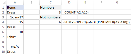
Sum if cell contains text
If you are looking for an Excel formula to find cells containing specific text and sum the corresponding values in another column, use the SUMIF function.
For example, to find out how many dresses are in stock, use this formula:
Where A2:A10 are the text values to check and B2:B10 are the numbers to sum.
Or, put the substring of interest in some cell (E1), and reference that cell in your formula, as shown in the screenshot below: 
To sum with multiple criteria, use the SUMIFS function.
For instance, to find out how many blue dresses are available, go with this formula:
Or use this one:
Where A2:A10 are the cells to check and B2:B10 are the cells to sum. 
Perform different calculations based on cell value
In our last tutorial, we discussed three different formulas to test multiple conditions and return different values depending on the results of those tests. And now, let’s see how you can perform different calculations depending on the value in a target cell.
Supposing you have sales numbers in column B and want to calculate bonuses based on those numbers: if a sale is over $300, the bonus is 10%; for sales between $201 and $300 the bonus is 7%; for sales between $101 and $200 the bonus is 5%, and no bonus for under $100 sales.
To have it done, simply multiply the sales (B2) by a corresponding percentage. How do you know which percentage to multiply by? By testing different conditions with nested IFs:
=B2*IF(B2>=300,10%, IF(B2>=200,7%, IF(B2>=100,5%,0)))
In real-life worksheets, it may be more convenient to input percentages in separate cells and reference those cells in your formula:
The key thing is fixing the bonus cells’ references with the $ sign to prevent them from changing when you copy the formula down the column. 
Excel conditional formatting if cell contains specific text
If you want to highlight cells with certain text, set up an Excel conditional formatting rule based on one of the following formulas.
Case-insensitive:
Case-sensitive:
For example, to highlight SKUs that contain the words «dress», make a conditional formatting rule with the below formula and apply it to as many cells in column A as you need beginning with cell A2:
=SEARCH(«dress», A2)>0 
Excel conditional formatting formula: if cell contains text (multiple conditions)
To highlight cells that contain two or more text strings, nest several Search functions within an AND formula. For example, to highlight «blue dress» cells, create a rule based on this formula:
=AND(SEARCH(«dress», A2)>0, SEARCH(«blue», A2)>0) 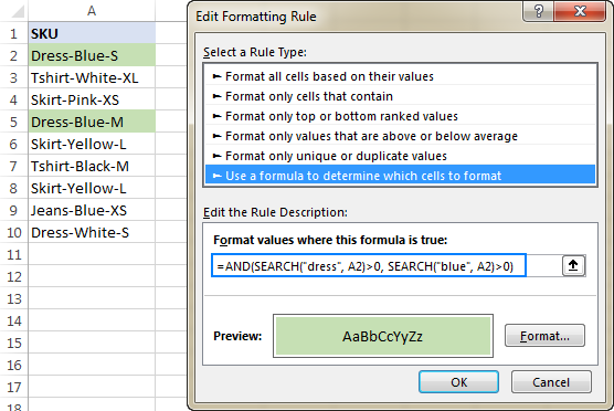
If cell contains certain text, remove entire row
In case you want to delete rows containing specific text, use Excel’s Find and Replace feature in this way:
- Select all cells you want to check.
- Press Ctrl + F to open the Find and Replace dialog box.
- In the Find what box, type the text or number you are looking for, and click the Find All
- Click on any search result, and then press Ctrl + A to select all.
- Click the Close button to close the Find and Replace
- Press Ctrl and the minus button at the same time ( Ctrl — ), which is the Excel shortcut for Delete.
- In the Delete dialog box, select Entire row, and click OK. Done!
In the screenshot below, we are deleting rows containing «dress»: 
If cell contains, select or copy entire rows
In situations when you want to select or copy rows with relevant data, use Excel’s AutoFilter to filter such rows. After that, press Ctrl + A to select the filtered data, Ctrl+C to copy it, and Ctrl+V to paste the data to another location.
To filter cells with two or more criteria, use Advanced Filter to find such cells, and then copy the entire rows with the results or extract only specific columns.
This is how you manipulate cells based on their value in Excel. I thank you for reading and hope to see you on our blog next week!
Practice workbook
You may also be interested in
Table of contents
I would appreciate any help
I have a spreadsheet with scores from events. Each person has participated in four events and they have four separated scores. I have assigned a point system for scores (i.e a 9 would give someone 20 points). is there a formula(function) that can look at the four cells of scores, determine if they qualify for points assigned and sum them into one cell of total points?
Hello!
To find multiple results that match the condition, use these guidelines and examples: How to Vlookup multiple values in Excel with criteria
If you need to calculate an sum by a condition, use the SUMIF function.
I have read ur example in «Perform different calculations based on cell value». Is there another simple way formula without using IF?
Because i have many tier in «Bonus». it too long if using IF
Hi!
If you have a lot of conditions, use the IFS logic function. Read more in this article: The new Excel IFS function instead of multiple IF.
Many thanks for your reply. i’ll try look IFS function
On our employee vacation tracker, I’m trying to add up any cells with a «V» value over multiple sheets. When I used the =COUNTIF(January!C7:AG7,»*V*») it works for that sheet, but I’m not sure what the formula is to add all the sheets for January to December for each employee. I’ve tried this =COUNTIF(January:December!C7:AG7,»V») but I get an error. Thanks in advance for your help!
Hello!
Unfortunately, your formula will not work. Here are the functions you can use to refer to the same cell or range in multiple sheets: Excel functions supporting 3-D references.
I have a table with data validation for the payment frequency to keep the spelling consistent.
I have table columns: Category, Payment Frequency (look up column), Payment Amount, Monthly Amount (cell multiplied or divided in formula)
Calculation: When I enter the payment frequency and the payment amount, I want to calculate the monthly payment amount.
Payment Frequency is calculated: monthly (*1), yearly (/12), bimonthly (*6), biweekly (*26/12), quarterly (*4/12), One time payment (*0) [I am not sure how to make that fit with the other payment options. ]
* Sorry, thought I had that clearer. The Monthly Amount is the cell in which I will insert the formula. The payment amount is the one multiplied/divided based on the payment frequency. The multiplier/divisor is in the brackets after the given payment frequency.
Hi!
Based on your description, it is hard to completely understand your task. However, I’ll try to guess and offer you to try the SUMIFS function. For more information, please visit: Excel SUMIFS and SUMIF with multiple criteria – formula examples. If this does not help, explain the problem in detail.
I am trying to tally attendance at programs based on age groups and type of program. I’m having issues getting a 0 total of the Sum of 3 age groups if type column contains «X» text. Using similar =SUMIF(D2:D6,»On»,A2:C6) I get 23 to display in formula’s box, but for =SUMIF(D2:D6,»Off»,A2:C6) I get zero instead of 15? Please help me find & fix my error.
Sample of spreadsheet:
A B C D
R1 Juv Teen Adult On/Off Site
R2 5 0 0 On
R3 0 7 6 On
R4 0 0 3 Off
R5 10 0 2 Off
R6 0 4 1 On
On Site total = 23
Off Site total = 15
Hello!
In the SUMIF formula, all ranges must be of the same dimension. Yours are different. For more information, please visit: How to use SUMIF function in Excel with formula examples.
I’m stumped on auto populating a cell. What I want to input is if sheet 2, column A contains any of the same text as sheet 1, column A. Then sheet 2 column 3 will auto populate the same numbers that are showing on Sheet 1, column 3.
Hello!
If I understand your task correctly, the following tutorial should help: VLOOKUP across multiple sheets in Excel with examples.
HI, Im looking for help with formatting a cell. So I want cell $G$277 to show as cell multiplied by .9789 if cell $E$277 shows as «bio». could anyone tell me how to input this please? thanks
sorry i wrote this incorrectly i mean to type
HI, Im looking for help with formatting a cell. So I want cell $G$277 to show as cell $H$277 multiplied by .9789 if cell $E$277 shows as «bio». could anyone tell me how to input this please? thanks
Hi!
With formatting, you cannot change the value of a cell. To change the value of a cell by condition, use the IF function.
Hi, thanks for the reply. I know i cant change the value of a cell, im trying to populate a cell based on an equation/formula based on a result from another cell but i just dont know how to write the equation.
I want for instance cell A1 to show the result of cell B1 multiplied by 0.9789 as the «true» if cell C1 has the word «Bio» in it, does that make sense? thanks
Hi!
Cell A1 can contain either a value or a formula like this:
Hi, I’ve tried that but nothing happens in the cell even though C1 has the word in it and B1 has a number populated in it ready for the formula to make the result in cell A1
I need to do this through conditional formatting as there is other information inputted that i need it to ignore
Hi!
As I already wrote to you, using conditional formatting it is impossible to change the value in the cell.
i have this formula in a column =IF(COUNTIFS($I:$I,I2,$Z:$Z,»YES»),»OK»,»NO») the «YES» result corresponds to another value as a result of look up on the other sheet. i would like to populate that lookup value on the entire next column.
how to do it please. thanks in advance
Hi!
Sorry, it’s not quite clear what you are trying to achieve. Could you please describe it in more detail?
hi sorry for that.. here in my table below, i have two groupings. In the column C is where my formula as =IF(COUNTIFS($A:$A,A2,$C:$C,»YES»),»OK»,»NO»). All the YES value in Column C ( as Apple and Milk ) is from my table in the other sheet with corresponding value of Fruits and Drinks. I need to put all the lookup result in the all cell for each group in Column E. how can i do it.
Column A Column B Column C Column D Column E
IMS Cherry No Ok Fruits
IMS Apple Yes Ok Fruits
IMS Soda No Ok Fruits
IMS2 Soda No Ok Drinks
IMS2 Milk Yes Ok Drinks
IMS2 Orange No Ok Drinks
Hi!
Your explanations are still not clear. I assume that your formula is not in C but in column D. This formula determines if there are duplicate rows. The results of this formula do not match with your data.
Explain «lookup result» — what are you looking for and where.
As it’s currently written, it’s hard to tell exactly what you’re asking.
Apologies.. yes my formula is n Column D where it becomes «OK» as it found «Yes» in Column C.
First is , i have to vlookup the DATA in Column B from the other sheet so i can have the YES or NO in Column C ( like the APPLE and Milk as YES value in Column C )
Second, in Column D is where i have the IF formula whether «OK» or «NO» .
Third, in Column E, something i need to get done. The YES value in Column C ( as APPLE and MILK corresponds to Fruit and Drink from other Sheet (so vlookup Apple will give me a result value of Fruit.)
so here in Column E i need to have a condition that if after the vlookup, the result value ( as Fruit ) will be filled in the certain cell per Group ( 3 cell per Column A groupings as per my sample.)
my apologies if i cant still explain it clearly here.. many thanks!
Hi!
To check data from column B on another sheet, you can use the MATCH function like this:
I don’t understand what you want to do in column E.
i can check the data from column B on another sheet by the this formula
sheet2:
Column A Column B
Apple Fruits
Milk Drinks
so in Sheet1: Column E
What i want in Column E is to fill the cell with «Fruits» without the #N/A
and this is what i am having now in Column E (based on my table above)
instead i want to have the formula which will gives me this.
Column E
Fruits
Fruits
Fruits
Drinks
Drinks
Drinks
Need help writing a formula to calculate percentage of invoices validated with payment dates. Essentially, we want to write a formula to generate a count of the cells with dates in them, and to exclude the cells with nothing. Based off this, we are building a gauge chart to depict the percentage of invoices validated. Min value would = 0 and Max value would = total invoices (with & without dates) and this formula would be the main data point showing percentage of invoices ONLY with payment dates tied to them.
Any tips/advice are greatly appreciated!
Hello!
To count the number of cells with dates, try this instruction: Count if blank or not blank. I hope it’ll be helpful. If this is not what you wanted, please describe the problem in more detail.
I’m looking for a formula that counts the number of cells that contain ANY text, and sum the number of cells in a cell below.
I need to sumerize how many clients each day, and obviously they all have diffrent names, and its always changing. As a bouns I’d like to enter that sum into another spreadsheet, on a specific days cell. the 2nd part is not vital. I’m running a homeless shelter and finding this formula stuff hard to absorb, lol.
So I figured the first part out, and feel free to ignore the second. I’m trying to learn everything and have a couple course type files, and now found this jem. Thanks for helping people out so much, very kind of you all.
Hi!
Pay attention to the first paragraph of the article above.
It covers your case completely.
Is possible to sum all WA11?
WA11 4
AdBlue 1, WA11 2
AdBlue 3, WA11 3, shift 4
. and everything is in one column
Hi!
You can’t do math with text. Split text into columns as described in this guide: How to split text string in Excel by comma, space, character or mask. You can also use the new Excel TEXTSPLIT function to split text. Then use the SUMIF function to calculate the sum by condition.
I have a time sheet that has a job code that I would like excel to reference to add up the hours that each employee has worked for that job to come up with the total hours worked on that job for the week.
So, if there is a letter in one cell, I want excel to take the numbers from another cell and add them all together for every occurrence of that letter in the table.
Hello!
To calculate the amount by conditions, use the COUNTIFS function. You can find the examples and detailed instructions here: Excel COUNTIFS and COUNTIF with multiple AND / OR criteria.
I’m not sure that is the correct formula.
Jobsite Code Job Total
AB A
CD C
FG D
Employee Mon Job Tue Job Wed Job
John 6 A 8 C 7 D
Joe 9 C 7 A 8 C
Taking the table above, I want Excel to look for A and add the hours from the corresponding cell; so, there’s an A in D7 and F8, I want Excel to add the hours in D6 (6 hours) and F7 (7) together for total hours worked on job A
I hope I answered your question.
What formula would I use (or is there one) to total the hours employees took to take certain staff training requirements (example table below):
A B C D E F G
1 Employee Name Course 1 Course 2 Course 3 Course 4 Course 5 Hours Completed
2 Course Length 3.25 1.25 1.50 1.00 0.75
3 Employee 1 10/17/22 10/12/22 10/12/22
4 Employee 2 10/16/22 10/04/22 10/12/22
5 Employee 3 10/17/22 10/13/22 10/13/22
6 Employee 4 10/17/22 10/17/22 10/11/22 10/11/22
Hi!
Based on your description, it is hard to completely understand your task. However, I’ll try to guess and offer you use SUMPRODUCT function.
Sorry the table didn’t come across very well, but that’s exactly the formula I needed. Thank you!
Is possible to sum this text?
Some text in cell. r=11
R=1,5. Some text in cell.
Sum all r=? and, that’s in one row.
Hello!
Here is the article that may be helpful to you: Extract number from text string.
Thank you very much
Hi i want to add following numbers which are present in a row
23,45,#N/A, 56,#N/A, 756.
Please suggest the formula to solve it.
Hi!
I don’t see any logic in your numbers. Try to look for a solution to the sequence of numbers in the article: SEQUENCE function in Excel — auto generate number series.
I’ve got the same issue I think Baiju is having, in that Excel isn’t clear on how you add up a series of columns or rows if some of the cells in the range have #NA or #NUM instead of a number.
I’ve got someone’s spreadsheet I’m trying to salvage. They’re trying to track the total invoices they process each month, amount of days to process each one, the number that are late (>30 days), and the $ amount for the invoices that are late. So, I’ve been using =DATEDIF and =IF(AND and =COUNTIF formulas to take a stab.
It’s cumbersome but would be working, except their spreadsheet includes all their invoices, including those that haven’t cleared yet. As a result I get #NUM! or #NA in those cells. When I try to sum the monetary values for the month (either =SUM or =COUNTIF) it fails because of the #NUM and #NA in the range. I haven’t been able to find an explanation on what to do when you’ve got non-numbers in a column you’re trying to add, so any advice you can provide would be appreciated. Thanks.
Hello!
Use the IFERROR function in formulas to avoid getting an error message. To calculate the sum, you can use the AGGEGATE function instead of the SUM function. If the second argument to this function is 6, then errors will be ignored.
I hope it’ll be helpful.
I need help to assign weights to text. For example, in the following response table,
Question No Response Weights
Q1 Red 1
Q2 Blue 2
Q3 Green 1
Q4 Red 2
Clearly, questions 2 and 4 are having higher importance. When commuting the response, it needs to read as
Red: (Q1*1+Q4*2) = 3
Blue: (Q2*2) =2
Green: (Q3*1) =1
Total =7 (not 4)
I’m trying to make a formula in which if an exact value is can get 4 different values in 4 different cells . Eg if A1=4 then B2=12, C2=199, D2 =122,E2=78
Hi!
We wrote many times that an Excel formula can change the value only in the cell in which it is written. You need to use a VBA macro.
Or use an IF formula in each cell.
Hi and thank you.
Stuck trying to work out formula for staff roster, whereby in a row of cells x 7 (one week) each shift worked (x 3 shifts, which equal 12 hours each) adds the sum of these shifts to a separate cell.
Eg.. Staff Name / Sum of Total Hrs / LD / / LD / LD
Should look like-
Staff name / 36 / LD / / LD / LD
This will actually be over 6- week roster, but just trying to get an idea of what to do in the above eg.
Thanks
Hi!
I’m not sure I got you right since the description you provided is not entirely clear. However, it seems to me that the formula below will work for you:
Use the COUNTIF function to count the number of specific values in seven cells.
I’d really appreciate help with a formula.
Column E is an IF statement and depending on a date range puts «YES» or «NO» in column E.
I’m trying to get a separate cell to provide the SUM of the number of «YES»s. SUM and SUMIF do not appear to work. For example, I have attempted the formula =SUMIF(E2:E20,»YES»). It incorrectly provides «0» as the answer. Is this because Column E is a separate formula itself. How do I get around this?
Your help is much appreciated.
Hello!
The SUMIF formula works with the results of formulas in the same way as with normal values. Your formula should work. Check what values are returned by your formulas in cells E2:E20. Perhaps there are extra spaces.
I would appreciate your help on a formula.
I am creating a vertical employee absence calendar in Excel (dates at the top, names on the side) with leave entered as text: holiday (H), half day holiday (HH), sick leave (S), and half day sick leave (SH).
I would like to add a row total for each person.
With COUNTA all entries = 1
So for e.g. H + S + HH should add up to 2.5 but COUNTA shows 3.
How can Excel add up different values for each type of text? So that that H = 1, HH = 0.5, S=1 and SH=0.5?
Very grateful for your help
Valerie
Many thanks for your help!
Hi!
The COUNTA function counts the number of cells. So it cannot return a fractional number. Replace letters with numbers using the IF function:
how I sum if I had 3 table
1 vendor (Samsung or Huawei)
2 Cell mode (ex Samsung I9500 series)
3 count
I used below formula but it count other vendor model as well
can you please support for the correction
Hi!
To calculate the sum of two criteria, use the SUMIFS function.
This should solve your task.
Hi
I need your support for correction of formula.
Please check below this formula is correct or not
=SUM((Sheet2!$D$8:$QC$11)*(—(Sheet2!$C$8:$C$11=’Cleaning details’!$D6))*(—(Sheet2!$D$4:$QC$4=’Cleaning details’!$C6))*(—(Sheet2!$D$3:$QC$3=’Cleaning details’!$E$4)))+SUM(Sheet2!$D$12:$QC$15)*(—(Sheet2!$C$12:$C$15=’Cleaning details’!$D6))*(—(Sheet2!$D$5:$QC$5=’Cleaning details’!$C6))*(—(Sheet2!$D$3:$QC$3=’Cleaning details’!$E$4))+SUM(Sheet2!$D$16:$QC$19)*(—(Sheet2!$C$16:$C$19=’Cleaning details’!$D6))*(—(Sheet2!$D$6:$QC$6=’Cleaning details’!$C6))*(—(Sheet2!$D$3:$QC$3=’Cleaning details’!$E$4))+SUM(Sheet2!$D$20:$QC$23)*(—(Sheet2!$C$20:$C$23=’Cleaning details’!$D6))*(—(Sheet2!$D$7:$QC$7=’Cleaning details’!$C6))*(—(Sheet2!$D$3:$QC$3=’Cleaning details’!$E$4))
Because this is not working in single cell.
Hi!
It is very difficult to understand a formula that contains unique references to your workbook worksheets. Hence, I cannot check its work, sorry.
Hi, my business gives commissions to our drivers (called “captains” as shown in the Excel screenshot). Their commission is 10% of the sale price of a surcharge they sell.
I want to track their daily commissions per captain and then total each daily commission for their weekly total commission per captain.
I already have their daily tracking set up to automatically calculate their daily commissions based on the prices of surcharges and tally of quantity sold for each.
My issue now is making the formula that automatically searches row P5 to T5 for instances of their unique name being written. Each time their name is written in that row indicates one working day with commissions made (total for each daily commission is in row P30 to T30) in their own column.
I would then like the same formula to have N34 to N36 autofill if there are captain’s names found in P5 to T5 (without duplicating their names) and then totaling their daily commissions specific to each captain’s name in the weekly totals at O34 to O36.
I hope this makes sense. Let me know if you need clarification.
I’ve tried for several hours to figure it out with various formulas but I’m not too versed in Excel so I’m hoping someone can help me out. Thanks in advance!
Sorry, there is no simple solution for your task. At least I do not know such 🙁
Hi,
SUMIF function is working for me but SUMIFS is not working even though I tried so many times. =SUMIFS(J2:J29,G2:G29,»Passive»,G2:G29,»Connector») is the formula which I am trying in my excel. I also have used * prior to text values but no result and instead its showing 0. I can’t understand why its showing 0. Kindly help.
Hello!
I can’t see your data and can’t check, but this formula should work
I recommend reading this guide: Excel SUMIF with multiple criteria (OR logic).
Hope this is what you need.
I have an Excel sheet where in column A i have various dates for sales over a three year period and in column B I have another column which contains text relating to the type of sale, either «Direct» or «Indirect» to indicate if the sale was a direct sale or through another party. I want to be able to count how many Direct or Indirect sales were made in each year. Can you help? I have tried combining the COUNTIF and COUNTIFS formulas but it’s not working. I can get the number of sales in each year by using the COUNTIFS formula but the problem starts when I try to extract the count in each year for each of Direct or Indirect by combining the two formulas. Thanks! Your website is amazing! I’ve managed to solve a lot of problems by checking your solutions.
Hello!
What formulas are you using? What’s not working in them? You must use the COUNTIFS formula with two conditions — Date and Sales Type.
Please have a look at this article — Excel COUNTIFS and COUNTIF with multiple AND/OR criteria
If they don’t work for you, then please describe your task in detail, I’ll try to suggest a solution.
What formula could I use to add up both numbers and letters in the same column? For example, I have 12 cells with values in the same column (the «x» respresents 1):
Before the numbers were added and we were only counting «x», we used this formula =COUNTIF(G73:G85,»=x»)
Now that numbers are also included, I am having trouble finding a formula that adds both «x» as 1 and the rest of the numbers.
Hello!
If I understand your task correctly, the following formula should work for you:
SUM function only adds numbers and ignores text.
I have two tabs:
First tab:
Column A Name
Column B Yes ( or No)
For example :
Column A Column B
Anna Yes
Lily No
If column B is value is Yes, I want to add column A value (Anna) to the other tab A1.
If column B is value is No, I don’t want to add column A value (Lily) into the other tab.
How to achieve that?
Hello!
You can use the guidelines and examples from the article: How to VLOOKUP multiple values in Excel with one or more criteria.
You can also use the FILTER function to get the values you want.
I hope my advice will help you solve your task.
I am having a really hard time trying to get the formula I need. The spreadsheet is for stock options. For easy example, column A are debits that it cost to open the contract. The adjacent cell in column B is the price I sell to close the contract. I have everything I need for the gain/loss and percentage taken. I am trying to figure out how I would calculate my true return? if for example I open a contract for -$500 and sell it for $750, I have a return of 50% on that specific row. However if I open another trade using that same $500 and then the $250 I captured for a trade as well, how would I calculate my overall return? It would want to calculate my return on $1250 instead of $750. Any help would be greatly appreciated.
Hi!
We are not stock specialists. If you have a specific question about the Excel formula, we will try to help.
Trying to make a formula using sumifs in B1 «lol» && C1 «wow
A1 blank cell (i want to put name text here which will be the reference of A2:A10)
B1 show the total lol
C1 show the total wow
A2:A10 Names
B2:B10 [sum_range]
C2:C10 text «Lol» or «wow»
I want to sum the value in B2:B10 if it meets the condition:
Sumif:
Condition 1 If A2:A10 is true (or same with the text I input in A1)
Condition 2 If C2:C10 «lol» or in «wow» category
e.q.
A1 «10/06»
B1 (if A1 is true A2;A10 sum the total 10/06 with lol
C1 sum the total 10/06 wow
Hello!
To find the sum of values for conditions, use the SUMIFS function.
If something is still unclear, please feel free to ask.
Hey Alex,
At the outset, very wonderfull site and informative.
I have the data in the following cols
Col A Col B
21-Sep-21 55
23-Sep-21 74
02-Oct-21 21
05-Oct-21 05
All I want to do is add the values apprearing for Sep and Oct as below
Sep’21 xxxxx
Oct’21 yyy
Hi!
I don’t understand what you want to do. Explain in more detail.
I am trying to find a formula to calculate cum GPA but will subtract the grades that have «TR» by it in the semester column. What formula if any would work for this?
EXAMPLE
Grade Hrs Points Semester
A 3 12 SP20
B 3 9 TR
C 2 4 FA21
D 1 1 TR
Hi!
Try using the AVERAGEIF function to calculate the average with conditions.
I need help with this formula. =SUMIF($D:$D,»*Wave 1*»,$F:$F)
Right now I want to add values from F if D says Wave 1 however if the the sum is 0 i want it to say TBD .. not sure how to do the TBD part
Hi!
What is TBD? Please describe your problem in more detail.
Hi,
I need to add values in alternative cells. eg: values in I5,K5,M5 and the sum should ignore text in those cells. Please suggest
In fact i would like to know whether excel can display the value of a cell in another cell by using an IF condition.
e.g value of A1 is «FLOWERS»
input text «FL» in B1
the result should be the value of A1 to be displayed in C1 if you put a condition that if the value of B1 = «FL»
is there any formula to solve this.
Hello!
You can learn more about IF function in Excel in this article on our blog.
I have a list of parts in column A, then i have a list of dates in column B
I want the formula to return how many times each part number has a date beside it
123456 1-jan-21
234567 5-jan-21
123456
123456 5-feb-21
so i would want this to return
123456 2
234567 1
Hello!
If I got you right, the formula below will help you with your task:
D1=»123456″
You can learn more about COUNTIFS function in Excel in this article on our blog
I hope it’ll be helpful.
Please help me figure this out. I have a spreadsheet of pupils’ scores on a test. I have put a ‘1’ in a cell if they got the question correct, a ‘0’ if incorrect and a ‘.’ if they didn’t attempt it. I have a separate list to the side which says the name of the topic next to each question number. I would like to generate a list of topics they need to practice for each pupil based on the questions they got wrong. How can I do this? For example, if they got question 8 and 10 incorrect and these questions were a multiplication and a division question I would like a list which says multiplication and division. Please help me figure this out!
Hello!
Please use the following array formula —
A3:C30 — your table, I3 — name, J3 — zero or «.» K3 — this formula.
Please have a look at this article — Vlookup multiple matches and return results in a row (Formula 2)
I hope I answered your question. If something is still unclear, please feel free to ask.
Hi Everyone, I would really like some help with this logic
I would like to create a formula in cell C2, if D2 = text «X» perform sum of A2 + B2, but if D2 = text «W» cell = just the value in B2
I hope this makes sense, TIA
Hi,
Please have a look at this article: Nested IF in Excel – formula with multiple conditions
It contains answers to your question
If all my cells contains value,(without blank) then I should get the output as T else F
Will anyone please help me out
What I’m looking for is a formula that will do the following:
If cell a1 contains specific text, then count cell a2.
I’ve tried all sorts of different options, but can’t get it to show the right count.
Hello!
You can check the text written in the cell using the ISTEXT function. Use it in an IF function statement. I don’t quite understand what «count cell a2» means.
Here is an example of what I’ve attempting. Perhaps this might help.
If in the range of data, X appears, then count the next cell after X (which would have A, B, or C in it).
Thank you for all the Information they are great. what i would like to dois:
I Have in column A a data validation that has X,Y Z and on a different sheet under X i have a list of names in a column as well as under Y ans Z. what I want, is when I choose for example X in column A, I want in column B automatically to copy all the names of the other sheet under X into the cells in column B into a column not row? please can you help me with this problem?
Hello, could you please help me to find formula that highlights the cell with specific text when the text is a list? Is this the correct way to do it in Conditional Formatting (by formula)?
=ISNUMBER(MATCH($A$2,List,0))
when list is the range of list cells?
If this is the best way, Is there a way to copy this exact formatting to other cells (format painter doesn’t do the job)?
Thank you so much in advance.
Hello Ludmila!
If I understand your task correctly, the following conditional formatting formula should work for you:
where F2 is the first cell of the list cell range.
I hope it’ll be helpful.
Hello Alexander, thank you for your answer. Unfortunately, the formula you’ve suggested didn’t work for me, though the formula that includes range of cells containing the list works well.
My additional question was is there a way to apply the same conditional formatting formula to multiple cells. I mean is there a fast way to copy the conditional formatting formula that will be updated to other cells (eg A3, A4 and so on) instead of creating a new rule for every next cell? Thank you!
Hello!
I’m sorry the formula wasn’t useful to you. Apparently, we represent your data differently.
How to copy conditional formatting is described here.
I am looking to use a condition on one cell (A2=Kabul, then pick data from another sheet, K5) and the same condition will be repeated in one formula (A2=Laghman, A2=Logar. and then data will be picked from a different cell). How I can do it?
Hello Ebadullah!
I’m sorry but your task is not entirely clear to me.
For me to be able to help you better, please describe your task in more detail. Please let me know in more detail what you were trying to find, what formula you used and what problem or error occurred. Give an example of the source data and the expected result. It’ll help me understand it better and find a solution for you. Thank you.
Hi there,
How do I Sum out multiple SKUs when I keyed them in according to the warehouse racking layout?
Example :
A1 B1 C1 are the name of the SKUs, while A1 C1 has the same SKU.
A2 B2 C2 will be the Quantity of each SKU above.
How do I get the the sum of A2 and C2 in a separate list if we got 600 SKUs.
Thank you.
Please if cell b4 has a data of 24pcs and cell c4 has 34000.
I want to multiply the two cell together.
Please how can I go about this.
Thanks
Hello Gbenga!
If I understand your task correctly, the following formula should work for you
=LEFT(A1,LEN(A1) — FIND(«pcs»,A1)) * B1
Hope you’ll find this information helpful.
Hello George!
In order to extract all the characters after «UL9», use the formula below:
=RIGHT(A10, LEN(A1) — FIND(«UL9», A1,1) +1)
As for pulling the text before «UL9», here is the formula for this case:
=LEFT(A1, FIND(«UL9», A1 ,1) — 1)
BTW, there is a formula-free solution for this task called Extract Text tool. Check out its manual, I believe you’ll find it helpful: https://www.ablebits.com/docs/excel-extract-text/
How can I delete upon scanning a bar code, everything except the text that starts with UL9C0037365 value in a cell
01008568230065341119071521UL9C0037365
Thank you
george
Thank you so much for most helpful forumula
How do I have a cell calculate a sum if there’s a certain word or text in another cell? I.E. 12345*2% will only be calculated if say cell A5 was showing the word «No».
Thanks!
I need a formula that will search a specific cell (E2) or all of column E for a «key» word and then if found, take the date in A2 and add 30 days to it and put this all in B2.
Please let me know if this can be accomplished.
Thanks.
Did you find a solution for your issue? I am currently trying to find something similar. I need to find all people who are online and add their hours, ignoring those who are on leave etc, Can anyone help?
Thanks in advance
Hi,
Is there a solution for this?
Basically, I have month in one column and dollars in another. If I want the sum of all the dollars in June, July and Aaugust in a separate column. Is there a formula that does this. I am sure there is but cannot figure it out.
Month dollar sum
June 20
June 30
June 25
June 22
June 31 sum of June dollars
July 18
July 16
July 15
July 22
July 19 sum of July dollars
August 6
August 3
August 32
August 34
August 24 sum of Aug dollars
Any Help Apprecaiated:
Essentially I am trying to write a formula where if all cells in a column range contain a numerical value it will SUM them, but add a condition where if the column contains a text it will search for the text and instead of returning a SUM it will return «Not Complete».
Currently I am working with the following formula but cant seem to get it to work:
=IF(ISNUMBER(SEARCH(«Not Complete»,H4:$H2000)),»Not Complete»,SUM(H4:$H2000))
For Reference:
Column of values mixed with text containing «Not Complete»
$0.052000
$0.052000
$0.052000
$0.052000
Not Complete
Not Complete
Not Complete
Not Complete
$0.052000
$0.052000
$0.052000
Trying to make a formula where if a cell has the text «GMP 1» then show the value which is in the same row but from column A. Also this has to work over separate sheets.
So, for example, i need it to look through column C on sheet 1 for the word «GMP 1» but return the row value of Column A, and put the result on sheet 2. Currently i have multiple efforts at the formula and getting results where it adds up the values from A (which i dont want) or #value #n/a or just the count value of if it is true. Tried multiple different starting points (sumproducts/vlookup etc)
Did anyone ever answer you? I’m looking for the same solution and can’t figure it out for the life of me. Thanks!
C5=Q
D5=Q
E5=H
F5=H
G5=Q
H5=Q
I5=H
J5=Q
K5=H
L5=H
M5=H
N5=H
O5=Q
P5=Q
Q is the travel plan for onsite. for the above example its 7 weeks stays.
but the onsite trip would be 4. so i need to caluclate the trip count.
I want to have a successive cell count where the value is «Q»
For the above example it would be 4.
Thanks
Srini
I am trying to see if excel can search a column and automatically add up specific cells to come as close to without exceeding a specific number. Example: I have a 12′ (120″) piece of lumber and I need to cut that into as many posts as possible with little waste. So in the example below it would highlight cells (A1, A2, A5, A6) in a specific color, then in another color continue with the other cells (not previously selected) and perform the same function. Thanks for any help.
A1 13.5″
A2 25.75″
A3 54″
A4 32″
A5 16″
A6 64.75″
A7 10″
A8 12.5″
A9 11
I’m working on a spreadsheet where i would like for a formula to be created when any text is entered into the cell to the left. If you enter a company name in a cell it will then create a PO based off the job number (in one cell) & the cost code (another cell)
Cell B2 is My Job Number & Cell A14 is My Cost Code. =B2&-A15 give me a my PO (Job Number-Cost Code). Now i would like this to be created only when text is entered in the cell to the left.
All Example and conversation are helpful,but if u add language option in your web side so its so easy and convenient for me and others, and I think Its plus point about you..
kind regards
sarmad azim
How about if i have a column of numbers and i want to search for matching numbers that then contain text in another column that i want to highlight mismatched PART text string. i.e
A1 B1
1 1562544 Engine
2 1562544 Cam Shaft
3 1573333 Engine 2
4 1573333 Engine 2
5 1582444 Engine
6 1582444 Engine
7 1582444 Cam Shaft Fixing
8 1628738 Cam Shaft
9 1628738 Cam Shaft — Chrome
I would only want a return for the rows that contain conflicting information i.e 1562544 and 1582444 in this case, i do not mind if it is just rows 2 & 7 that are returned or all that mismatch i.e 1&2 and 5,6&7 . Worth noting that rows 8&9 i do not consider a mismatch (hence the need for a PART string match)
Hope that makes sense
A cell contains =IF(ISNUMBER(SEARCH(«Avox Production»,B60)),»1″,»»)
The statement enters a «1» in the cell when the word «Avox Production» is typed in another cell B60.
I have a range of cells with the statement listed above. What I need to do is gather the sum of all cells with «1» and populate the total of these cells into another worksheet.
I’ve tried =SUM(B60:B65,Data!B60:B65) but nothing populates in the cell.
What is the cell address for the cell containing the formula:
=IF(ISNUMBER(SEARCH(«Avox Production»,B60)),»1″,»»)
That cell address will contain the «1» or «»
Sum that column to get your values
I need to do something along the lines of «If cell contains text «ab» then perform calculation (D10-0.15)-120)» basically I need the number showing in that cell to either be calculated using one formula or another. not sure how to structure this or if it’s possible. Thanks in advance!
Daniel:
You will use the SUMIF function including the optional sum_range. Where the data is in columns J, K and L enter this in L2:
=SUMIF(K2:K5,»PM»,J2:J5)
You’re saying, «Sum the values in J2 thru J5 where the text in the adjacent cells K2 thru K5 is PM.» So, it’s range, criteria, sum_range.
I was hoping you could help me with a formula.
I would like to calculate a range cells in a row if text is «Something»
so:
A1 A2 B4:
2.5 PM 6.0 This pulls all the values from A1 that have PM in A2.
2 CE
2.5 CE
2 IPT
3.5 PM
I was hoping you could help me with a formula.
I would like to calculate a range cells in a row if text is «Something»
2.5 PM
2 CE
2.5CE
2 IPT
3.5 PM
What Excel function and how to use if I select a word in cell (with drop down list with few text) and I would like each selected text to return a different drop down list from different sheet?
I would like to select only cell with numerical value from row containing numerical and non-numerical value.
I’d like to use a sumifs type formula, but instead of summing numbers, I’d like to grab text (vlookup won’t work because I need to use multiple criteria). Any ideas?
how to do if the cell is a date, say: 1/1/2018, then to sum a row of numbers and add another number in a cell, e.g. a2:j2, +e20. If it is not the date (1/1/2018), then let it be blanked.
Thanks for responding Doug, but nothing there is helping this particular scenario.
How would I sum a filtered columns visible data by using another columns text, I need the below formula to count visible cells of a filtered column based on a word
Sorry, More specific. Same question
Trying to get the above formula to sum Visible cells in column D, currently it sums all cells
Column E contains text,»Immediately» is one of the choices.
Column D contains numeric values that need to be summed
based on the choice of the word «Immediately»
They are filtered.
Phil:
Svetlana has a very thorough article here on AbleBits that covers this topic.
Enter «sum only filtered (visible) cells» in the search box and you’ll see the link to the article.
I would like to highlight Equal no. of cells to the numeric value in some cell. i.e
if i put 5 in cell no. A1, then cell B1,C1,D1,E1,F1 Shall be filled in red colour.
how to do it pls help
Krishna Das:
Sorry, I think the only way to do what you want is by writing some VBA code. That’s beyond the scope of this blog.
How To Highlight Row If Cell Contains Text/Value/Blank In Excel
Источник