If contains part of text excel

Let’s say you want to ensure that a column contains text, not numbers. Or, perhapsyou want to find all orders that correspond to a specific salesperson. If you have no concern for upper- or lowercase text, there are several ways to check if a cell contains text.

You can also use a filter to find text. For more information, see Filter data.

Find cells that contain text

Follow these steps to locate cells containing specific text:

1. Select the range of cells that you want to search.

   To search the entire worksheet, click any cell.

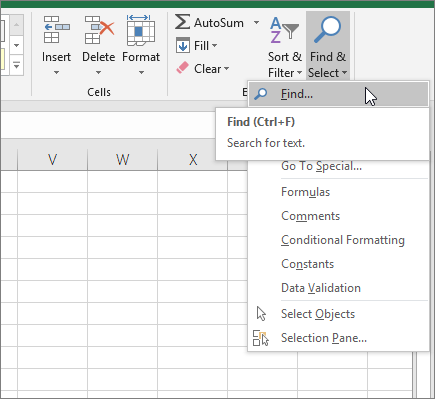
2. On the Home tab, in the Editing group, click Find & Select, and then click Find.

   

3. In the Find what box, enter the text—or numbers—that you need to find. Or, choose a recent search from the Find what drop-down box.

   Note: You can use wildcard characters in your search criteria.

4. To specify a format for your search, click Format and make your selections in the Find Format popup window.

5. Click Options to further define your search. For example, you can search for all of the cells that contain the same kind of data, such as formulas.

   In the Within box, you can select Sheet or Workbook to search a worksheet or an entire workbook.

6. Click Find All or Find Next.

   Find All lists every occurrence of the item that you need to find, and allows you to make a cell active by selecting a specific occurrence. You can sort the results of a Find All search by clicking a header.

Note: To cancel a search in progress, press ESC.

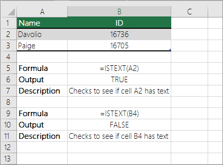
Check if a cell has any text in it

To do this task, use the ISTEXT function.

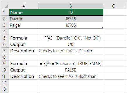
Check if a cell matches specific text

Use the IF function to return results for the condition that you specify.

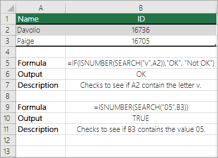
Check if part of a cell matches specific text

To do this task, use the IF, SEARCH, and ISNUMBER functions.

Note: The SEARCH function is case-insensitive.

Here is the Excel formula to Check If Cell Contains Partial Text. You can se this formula to determine the cell contains partial text and Count, Sum and do further processing.

Excel if cell contains partial text

Below Formula will check if cell contains partial text. It will return ‘Yes’ if it contains the partial text, ‘No’ if not found.

=IF(COUNTIF(A2,"*PartialText*"),"Yes","No")

This formula will check for the partial text in cell A2 and returns ‘Yes’ if found, returns ‘No’ if not found. You can return True, False if required as shown in the given formula.

=IF(COUNTIF(A2,"*PartialText*"),TRUE,FALSE)

Excel if cell contains partial text wildcard

Following are the useful wildcards to help in matching the partial text in excel formulas, and very useful to check if a cell contains partial text in Excel.

Asterisk (*)

You can use Asterisk (*) to match zero or more characters. Check the examples below:

• 1. Formula to check Excel if cell contains partial text, which should end with partial text
  =IF(COUNTIF(A2,"*PartialText"),TRUE,FALSE)

Here, * is the wildcard character preceding to the partial text.

• 2. Formula to check Excel if cell contains partial text, which should begins with partial text
  =IF(COUNTIF(A2,"PartialText*"),TRUE,FALSE)

Here, * is the wildcard character following the partial text.

• 3. Formula to check Excel if cell contains partial text, which contains the partial text at any position in the cell
  =IF(COUNTIF(A2,"*PartialText*"),TRUE,FALSE)

Here, * is the wildcard character following and preceding to the partial text.

Question mark (?) – one character

You can use Question mark (?) to match any one character. Check the examples below:

• 4. Formula to check Excel if cell contains partial text, cell should end with partial text and only preceding any one character.
  =IF(COUNTIF(A2,"?PartialText"),TRUE,FALSE)

5. Formula to check Excel if cell contains partial text, cell should begin with partial text and followed by any 3 character.
=IF(COUNTIF(A2,"PartialText???"),TRUE,FALSE)

Share This Story, Choose Your Platform!

4 Comments

1. Chris
   July 17, 2022 at 10:43 pm — Reply

   Hi, thanks for sharing this great tutorial. I have a question, how do you add multiple countifs in the same formula ? For example, if a cell contains some text, then display this…but if it contains another text, then display something else ? thanks!

   • PNRao
     September 11, 2022 at 6:44 am — Reply

     =IF(COUNTIF(A2,"*MyText*"),"String1-Yes",IF(COUNTIF(A2,"*AnotherText*"),"String2-Yes","No"))
     

2. JM
   December 2, 2022 at 9:36 pm — Reply

   Can I use this formula for more than 4 countifs in the same formula? if so can you show the formula?

   • PNRao
     December 5, 2022 at 11:24 am — Reply

     If you wants to count based on multiple criteria, you can use one CountIFS formula with multiple criteria. Please let us know your requirement, so that we can help you!

Smart searching makes the whole search process a breeze and that’s smart stuff for you, making everything easy breezy. As your search gets specific, the process gets more complicated and if you don’t employ the right techniques, you’ll find yourself having a bad fishing day in a ginormous Excel sea. See if you can get it right the first time with what we have planned for you here today.

Your learning today comprises checking cells for partial text using the SEARCH, COUNTIF, and MATCH functions along with other functions to control the outcome. Find out how to use wildcard characters to aid the search. We’ll use a case example to give the explanations a visual touch.

Case Example

Enlisted ahead in the example shot, we have our stock of fragrances. The fragrances are alphabetically sorted by name and the slight problem here is that the brand is also mentioned in the same cell. Now if we are to find fragrances according to a brand, we can’t do it as easily.

A start can be to split the brands from the names into a separate column but even then, we have a problem. If we alphabetically sort the brand names and search for a fragrance by Armani, our search will turn up pointless because the fragrance is listed by the name of Giorgio Armani and would be lying in the range of G while we’d be searching the brands with A as the initials.

So we need something a little more foolproof for our searches and we’ve expounded these ideas ahead in this tutorial.

Let’s get checking!

Using SEARCH Function

Partial text in a cell can be checked with the SEARCH function. The SEARCH function searches a cell for a given value and returns the position of the character at which the value is found. That’s how the SEARCH function will work on its own but there are ways to use the SEARCH function to expand its usability.

We can better look into this with an example so let’s merge our case example with the SEARCH function and apply the formula below:

=IF(ISNUMBER(SEARCH("Chanel",B3)),"Yes","-")

First we’ll talk about the SEARCH function. We want to find fragrances by Chanel in our stock and we have fed this brand name in the formula. The point of search is column B hence, the first cell to search is B3. Technically this should be enough, right? Let’s apply just the SEARCH function and see if it works:

Now that works… partially. The SEARCH function returns the position of the character where Chanel is found i.e. the 9th character. Since SEARCH couldn’t return the character’s position in the first instance (because B3 doesn’t contain the value «Armani»), it results in the #VALUE! error. While the SEARCH function on its own does something to give us the idea that the searched value is there, we need something more suitable for our spreadsheets.

Incoming: the ISNUMBER function. ISNUMBER returns TRUE when the provided value is a number and FALSE when it isn’t. This way, the ISNUMBER function will result in TRUE when SEARCH results in a numeric value and FALSE otherwise.

But we’re going for further prominence in the results and that’s why we’ve wrapped everything in the IF function. The IF function will yield a «Yes» upon finding «Chanel» as part of the cell value. Otherwise it will yield a dash «-«

With more clarity, we can easily see that we have 3 Chanel fragrances in stock.

Notes:

The SEARCH function doesn’t require a wildcard asterisk but a wildcard question mark can be used to replace a single character. Find out what a wildcard character is in the COUNTIF function section.

The SEARCH function is not case-sensitive. Switch it out with the FIND function for a case-sensitive option.

Checking Two Values

Checking our stock for Chanel was one value. Let’s also search for Gucci fragrances because why not? For searching two values, we will need the OR function. The OR function returns TRUE if any of the specified conditions are met and FALSE if none are met. Now see the formula with the SEARCH function for checking if a cell contains either of the two values:

=IF(OR(ISNUMBER(SEARCH("Chanel",B3)),ISNUMBER(SEARCH("Gucci",B3))),"Yes","-")

We’re finding two values so the formula has 2 SEARCH formulas; one with Chanel as the search value and one with Gucci. Both the SEARCH formulas are controlled by the ISNUMBER function. The OR function is fed with two conditions; find Chanel or find Gucci. If either is found, the IF function makes sure that «Yes» is returned. Else, a dash is returned.

Note: Suppose instead of finding two values in separate cells, you want to find two values in the same cell. E.g. we’re unable to recall the full name of a fragrance by Chanel but remember that the name included «de». In that case, the OR function will be replaced by the AND function and the search values will be «Chanel» and «de».

=IF(AND(ISNUMBER(SEARCH("Chanel",B3)),ISNUMBER(SEARCH("de",B3))),"Yes","-")

Using COUNTIF Function

An alternative to the SEARCH function for checking partial text in a cell is the COUNTIF function. The COUNTIF function is used to count the cells that meet a given condition. COUNTIF makes a lighter formula for finding partially matching text since the ISNUMBER function can be dropped.

The added touch is, however, having to use a wildcard character to match zero or more characters. In the coming sections, we’ll show you how to use the wildcard characters (the asterisk and question mark) within the COUNTIF function to check if a cell contains certain text.

Wildcard Characters

With Asterisk

The COUNTIF function needs to be triggered for searching part of the text in a cell with the asterisk in the formula. The asterisk acts as a replacement for zero or more characters and without it, the formula will search a cell containing just search text instead of searching a cell that includes the search text. The asterisk will be placed depending on the position of the text you want to find within the cell. Here’s a little helper:

Criterion	Parameter in the formula
Find text at the beginning of a cell	«text*»
Find text in the middle or anywhere in the cell	«*text*»
Find text at the end of a cell	«*text»

Judging from the above, the asterisk can also be placed at the end of Chanel if we’re unsure of any text after it in the cell. A safer bet will be to enclose the search text in asterisks because the presence of one can always account for zero characters but the absence will mean that there is no text.

Let’s proceed to the formula now so you can see how this works:

=IF(COUNTIF(B3,"*Chanel"),"Yes","-")

The COUNTIF function is to return 1 for a cell containing «*Chanel». The asterisk is placed before the text of interest because we know that the brand name will be the last part of the text in the cell. If the cell does not contain Chanel as the last of the text, COUNTIF will return 0.

To customize 1 and 0, we have added the IF function in the formula to replace these numbers with «Yes» and «-» respectively. These are the results:

Search a Range

In the case above, we were seeing which fragrances by Chanel were in stock. If we were only out to check whether the stock contained any Chanel fragrances at all, without specificity, we can apply the COUNTIF function to the whole range in the dataset and get a single cell result in return. In Excel words, the COUNTIF function works on a range as well as a single cell. Use this formula to check a range for partial matching:

=IF(COUNTIF(B3:B12,"*Chanel"),"Yes","-")

The only thing we have changed in this formula is the cell reference from B3 to the range B3:B12. The formula searches this range for cells that contain Chanel as the ending text. Since there are 3 cells in this range that meet this condition, the formula gives us a «Yes» in a single cell.

With Question Mark

Another wildcard character with an interesting characteristic is the question mark. While the asterisk can signify multiple characters, a single question mark signifies a single character and more than one can be used.

Let’s draw from our case example. We are certain there is a Lancome fragrance in our stock but can’t quite remember what spelling the entry has been made with. Was it Lancôme or Lancome? Don’t sweat it. It’s just the O causing dubiety and we can replace it with a question mark wildcard. Use a formula like this to check for partial matching using a wildcard question mark:

=IF(COUNTIF(B3,"*Lanc?me"),"Yes","-")

Only changing our search text in this formula, the rest is the same COUNTIF we were using earlier. Now we are searching for a Lancome fragrance with a leading asterisk because the remaining text is before the brand name in the cell. The dubious «o» in Lancome has been replaced with a question mark.

Applying this formula to all the fragrances in our dataset, we have one «Yes» returned for B11, solving our mystery spelling as Lancôme.

Notes:

The COUNTIF function works for ranges too so it can also be applied as a range formula, depending on what your requirement is.

Using MATCH Function

The last option for checking a cell that may contain your search text in part is the MATCH function. The MATCH function checks an array for a value and returns the position of the cell in that array. We can work with that. If the position of the cell in the array is what we insist on, then we can do with using just the MATCH function. But we’re finding a specific text in a range so we’ll throw more spanners into the works. Keep reading!

Wildcard Characters

With Asterisk

With the MATCH function, we also need to use the asterisk as a wildcard. We require other functions like in this formula ahead:

=IF(ISNA(MATCH("*Chanel*",B3:B12,0)),"Not Found!","Found")

The MATCH function has been equipped with Chanel as the first parameter enclosed in two asterisks to replace possible text. The lookup array is B3:B12 and 0 has been entered to find an exact match. When the search text cannot be found, MATCH will result in a #N/A error and for finding every match, 1 will be returned.

To channel #N/A and 1 into TRUE and FALSE, the ISNA function has been added in the formula. the ISNA function returns TRUE when a value is #N/A. Now the TRUE and FALSE are in guise with «Not Found!» and «Found» by the IF function respectively.

The MATCH function picked up on 3 cells that contain the text Chanel. ISNA checks for an #N/A error. Since MATCH’s result is 3, there is no #N/A error – leading to FALSE. The value for FALSE as per the IF function is «Found». The indication is that the search text Chanel has been found in the range B3:B12.

The same formula can be used with the range excluded and relative cell reference included to find the exact cells that contain the matching text:

=IF(ISNA(MATCH("*Chanel*",B3,0)),"Not Found!","Found")

With Question Mark

Now let’s see how to use the question mark as a wildcard character with the MATCH function for finding partial text in a range.

=IF(ISNA(MATCH("*Lanc?me",B3:B12,0)),"Not Found!","Found")

With the same lineup of the MATCH, ISNA, and IF functions, we’ve entered the search text with a wildcard question mark to find Lanc?me in B3:B12. And good news, it has been found.

Open up the results by using a cell reference instead of the range to specifically find the cell that contains the Lanc?me fragrance:

=IF(ISNA(MATCH("*Lanc?me",B3:B12,0)),"Not Found!","Found")

One more thing this tutorial contains is the end of the tutorial so we’re heading out of finding partial matches in text in Excel. But if this is new for you, get cracking with some text search experiments and before you’re ready to head out, we’ll be back with more Excel stuff to crack. You can count on us for that!

In this example, the goal is to test a value in a cell to see if it contains a specific substring. Excel contains two functions designed to check the occurrence of one text string inside another: the SEARCH function and the FIND function. Both functions return the position of the substring if found as a number, and a #VALUE! error if the substring is not found. The difference is that the SEARCH function supports wildcards but is not case-sensitive, while the FIND function is case-sensitive but does not support wildcards. The general approach with either function is to use the ISNUMBER function to check for a numeric result (a match) and return TRUE or FALSE.

SEARCH function (not case-sensitive)

The SEARCH function is designed to look inside a text string for a specific substring. If SEARCH finds the substring, it returns a position of the substring in the text as a number. If the substring is not found, SEARCH returns a #VALUE error. For example:

=SEARCH("p","apple") // returns 2
=SEARCH("z","apple") // returns #VALUE!

To force a TRUE or FALSE result, we use the ISNUMBER function. ISNUMBER returns TRUE for numeric values and FALSE for anything else. So, if SEARCH finds the substring, it returns the position as a number, and ISNUMBER returns TRUE:

=ISNUMBER(SEARCH("p","apple")) // returns TRUE
=ISNUMBER(SEARCH("z","apple")) // returns FALSE

If SEARCH doesn’t find the substring, it returns an error, which causes the ISNUMBER to return FALSE.

Wildcards

Although SEARCH is not case-sensitive, it does support wildcards (*?~). For example, the question mark (?) wildcard matches any one character. The formula below looks for a 3-character substring beginning with «x» and ending in «y»:

=ISNUMBER(SEARCH("x?z","xyz")) // TRUE
=ISNUMBER(SEARCH("x?z","xbz")) // TRUE
=ISNUMBER(SEARCH("x?z","xyy")) // FALSE

The asterisk (*) wildcard matches zero or more characters. This wildcard is not as useful in the SEARCH function because SEARCH already looks for a substring. For example, it might seem like the following formula will test for a value that ends with «z»:

=ISNUMBER(SEARCH("*z",text))

However, because SEARCH automatically looks for a substring, the following formulas all return 1 as a result, even though the text in the first formula is the only text that ends with «z»:

=SEARCH("*z","XYZ") // returns 1
=SEARCH("*z","XYZXY") // returns 1
=SEARCH("*z","XYZXY123") // returns 1
=SEARCH("x*z","XYZXY123") // returns 1

This means the asterisk (*) is not a reliable way to test for «ends with». However, you an use the the asterisk (*) wildcard like this: 

=SEARCH("x*2*b","AAAXYZ123ABCZZZ") // returns 4
=SEARCH("x*2*b","NXYZ12563JKLB") // returns 2

Here we are looking for «x», «2», and «b» in that order, with any number of characters in between. Finally, you can use the tilde (~) as an escape character to indicate that the next character is a literal like this:

=SEARCH("~*","apple*") // returns 6
=SEARCH("~?","apple?") // returns 6
=SEARCH("~~","apple~") // returns 6

The above formulas use SEARCH to find a literal asterisk (*), question mark (?) , and tilde (~) in that order.

FIND function (case-sensitive)

Like the SEARCH function, the FIND function returns the position of a substring in text as a number, and an error if the substring is not found. However, unlike the SEARCH function, the FIND function respects case:

=FIND("A","Apple") // returns 1
=FIND("A","apple") // returns #VALUE!

To make a case-sensitive version of the formula, just replace the SEARCH function with the FIND function in the formula above:

=ISNUMBER(FIND(substring,A1))

The result is a case-sensitive search:

=ISNUMBER(FIND("A","Apple")) // returns TRUE
=ISNUMBER(FIND("A","apple")) // returns FALSE

If cell contains

To return a custom result when a cell contains specific text, add the IF function like this:

=IF(ISNUMBER(SEARCH(substring,A1)), "Yes", "No")

Instead of returning TRUE or FALSE, the formula above will return «Yes» if substring is found and «No» if not.

With hardcoded search string

To test for a hardcoded substring, enclose the text in double quotes («»). For example, to check A1 for the text «apple» use:

=ISNUMBER(SEARCH("apple",A1))

More than one search string

To test a cell for more than one thing (i.e. for one of many substrings), see this example formula.