If command in excel with and

Use AND and OR to test a combination of conditions

When you need to find data that meets more than one condition, such as units sold between April and January, or units sold by Nancy, you can use the AND and OR functions together. Here’s an example:

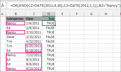
This formula nests the AND function inside the OR function to search for units sold between April 1, 2011 and January 1, 2012, or any units sold by Nancy. You can see it returns True for units sold by Nancy, and also for units sold by Tim and Ed during the dates specified in the formula.

Here’s the formula in a form you can copy and paste. If you want to play with it in a sample workbook, see the end of this article.

Use AND and OR with IF

You can also use AND and OR with the IF function.

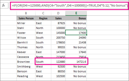
In this example, people don’t earn bonuses until they sell at least $125,000 worth of goods, unless they work in the southern region where the market is smaller. In that case, they qualify for a bonus after $100,000 in sales.

Let’s look a bit deeper. The IF function requires three pieces of data (arguments) to run properly. The first is a logical test, the second is the value you want to see if the test returns True, and the third is the value you want to see if the test returns False. In this example, the OR function and everything nested in it provides the logical test. You can read it as: Look for values greater than or equal to 125,000, unless the value in column C is «South», then look for a value greater than 100,000, and every time both conditions are true, multiply the value by 0.12, the commission amount. Otherwise, display the words «No bonus.»

Sample data

If you want to work with the examples in this article, copy the following table into cell A1 in your own spreadsheet. Be sure to select the whole table, including the heading row.

Источник

Function IF in Excel with a few examples of conditions

The logical IF statement in Excel is used for the recording of certain conditions. It compares the number and / or text, function, etc. of the formula when the values correspond to the set parameters, and then there is one record, when do not respond — another.

Logic functions — it is a very simple and effective tool that is often used in practice. Let us consider it in details by examples.

The syntax of the function «IF» with one condition

The operation syntax in Excel is the structure of the functions necessary for its operation data.

Let us consider the function syntax:

• Boolean – what the operator checks (text or numeric data cell).
• Value_if_TRUE – what will appear in the cell when the text or numbers correspond to a predetermined condition (true).
• Value_if_FALSE – what appears in the box when the text or the number does not meet the predetermined condition (false).

Logical IF functions.

The operator checks the A1 cell and compares it to 20. This is a «Boolean». When the contents of the column is more than 20, there is a true legend «greater 20». In the other case it’s «less or equal 20».

Attention! The words in the formula need to be quoted. For Excel to understand that you want to display text values.

Here is one more example. To gain admission to the exam, a group of students must successfully pass a test. The results are listed in a table with columns: a list of students, a credit, an exam.

The statement IF should check not the digital data type but the text. Therefore, we prescribed in the formula В2= «done» We take the quotes for the program to recognize the text correctly.

The function IF in Excel with multiple conditions

Usually one condition for the logic function is not enough. If you need to consider several options for decision-making, spread operators’ IF into each other. Thus, we get several functions IF in Excel.

The syntax is as follows:

Here the operator checks the two parameters. If the first condition is true, the formula returns the first argument is the truth. False — the operator checks the second condition.

Examples of a few conditions of the function IF in Excel:

It’s a table for the analysis of the progress. The student received 5 points:

• А – excellent;
• В – above average or superior work;
• C – satisfactory;
• D – a passing grade;
• E – completely unsatisfactory.

IF statement checks two conditions: the equality of value in the cells.

In this example, we have added a third condition, which implies the presence of another report card and «twos». The principle of the operator is the same.

Enhanced functionality with the help of the operators «AND» and «OR»

When you need to check out a few of the true conditions you use the function И. The point is: IF A = 1 AND A = 2 THEN meaning в ELSE meaning с.

OR function checks the condition 1 or condition 2. As soon as at least one condition is true, the result is true. The point is: IF A = 1 OR A = 2 THEN value B ELSE value C.

Functions AND & OR can check up to 30 conditions.

An example of using the operator AND:

It’s the example of using the logical operator OR.

How to compare data in two tables

Users often need to compare the two spreadsheets in an Excel to match. Examples of the «life»: compare the prices of goods in different bringing, to compare balances (accounting reports) in a few months, the progress of pupils (students) of different classes, in different quarters, etc.

To compare the two tables in Excel, you can use the COUNTIFS statement. Consider the order of application functions.

For example, consider the two tables with the specifications of various food processors. We planned allocation of color differences. This problem in Excel solves the conditional formatting.

Baseline data (tables, which will work with):

Select the first table. Conditional Formatting — create a rule — use a formula to determine the formatted cells:

In the formula bar write: = COUNTIFS (comparable range; first cell of first table)=0. Comparing range is in the second table.

To drive the formula into the range, just select it first cell and the last. «= 0» means the search for the exact command (not approximate) values.

Choose the format and establish what changes in the cell formula in compliance. It’s better to do a color fill.

Select the second table. Conditional Formatting — create a rule — use the formula. Use the same operator (COUNTIFS). For the second table formula:

Now it is easy to compare the characteristics of the data in the table.

Источник

Using IF with AND, OR and NOT functions

The IF function allows you to make a logical comparison between a value and what you expect by testing for a condition and returning a result if that condition is True or False.

=IF(Something is True, then do something, otherwise do something else)

But what if you need to test multiple conditions, where let’s say all conditions need to be True or False ( AND), or only one condition needs to be True or False ( OR), or if you want to check if a condition does NOT meet your criteria? All 3 functions can be used on their own, but it’s much more common to see them paired with IF functions.

Use the IF function along with AND, OR and NOT to perform multiple evaluations if conditions are True or False.

IF(AND()) — IF(AND(logical1, [logical2], . ), value_if_true, [value_if_false]))

IF(OR()) — IF(OR(logical1, [logical2], . ), value_if_true, [value_if_false]))

IF(NOT()) — IF(NOT(logical1), value_if_true, [value_if_false]))

The condition you want to test.

The value that you want returned if the result of logical_test is TRUE.

The value that you want returned if the result of logical_test is FALSE.

Here are overviews of how to structure AND, OR and NOT functions individually. When you combine each one of them with an IF statement, they read like this:

AND – =IF(AND(Something is True, Something else is True), Value if True, Value if False)

OR – =IF(OR(Something is True, Something else is True), Value if True, Value if False)

NOT – =IF(NOT(Something is True), Value if True, Value if False)

Examples

Following are examples of some common nested IF(AND()), IF(OR()) and IF(NOT()) statements. The AND and OR functions can support up to 255 individual conditions, but it’s not good practice to use more than a few because complex, nested formulas can get very difficult to build, test and maintain. The NOT function only takes one condition.

Here are the formulas spelled out according to their logic:

=IF(AND(A2>0,B2 0,B4 50),TRUE,FALSE)

IF A6 (25) is NOT greater than 50, then return TRUE, otherwise return FALSE. In this case 25 is not greater than 50, so the formula returns TRUE.

IF A7 (“Blue”) is NOT equal to “Red”, then return TRUE, otherwise return FALSE.

Note that all of the examples have a closing parenthesis after their respective conditions are entered. The remaining True/False arguments are then left as part of the outer IF statement. You can also substitute Text or Numeric values for the TRUE/FALSE values to be returned in the examples.

Here are some examples of using AND, OR and NOT to evaluate dates.

Here are the formulas spelled out according to their logic:

IF A2 is greater than B2, return TRUE, otherwise return FALSE. 03/12/14 is greater than 01/01/14, so the formula returns TRUE.

=IF(AND(A3>B2,A3 B2,A4 B2),TRUE,FALSE)

IF A5 is not greater than B2, then return TRUE, otherwise return FALSE. In this case, A5 is greater than B2, so the formula returns FALSE.

Using AND, OR and NOT with Conditional Formatting

You can also use AND, OR and NOT to set Conditional Formatting criteria with the formula option. When you do this you can omit the IF function and use AND, OR and NOT on their own.

From the Home tab, click Conditional Formatting > New Rule. Next, select the “ Use a formula to determine which cells to format” option, enter your formula and apply the format of your choice.

Edit Rule dialog showing the Formula method» loading=»lazy»>

Using the earlier Dates example, here is what the formulas would be.

If A2 is greater than B2, format the cell, otherwise do nothing.

=AND(A3>B2,A3 B2,A4 B2)

If A5 is NOT greater than B2, format the cell, otherwise do nothing. In this case A5 is greater than B2, so the result will return FALSE. If you were to change the formula to =NOT(B2>A5) it would return TRUE and the cell would be formatted.

Note: A common error is to enter your formula into Conditional Formatting without the equals sign (=). If you do this you’ll see that the Conditional Formatting dialog will add the equals sign and quotes to the formula — =»OR(A4>B2,A4

Need more help?

​​​​​​​

See also

You can always ask an expert in the Excel Tech Community or get support in the Answers community.

Источник

AND function

Use the AND function, one of the logical functions, to determine if all conditions in a test are TRUE.

Example

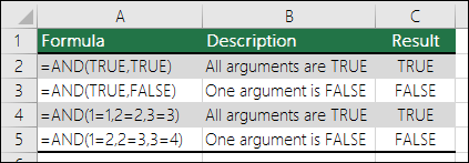
The AND function returns TRUE if all its arguments evaluate to TRUE, and returns FALSE if one or more arguments evaluate to FALSE.

One common use for the AND function is to expand the usefulness of other functions that perform logical tests. For example, the IF function performs a logical test and then returns one value if the test evaluates to TRUE and another value if the test evaluates to FALSE. By using the AND function as the logical_test argument of the IF function, you can test many different conditions instead of just one.

The AND function syntax has the following arguments:

Required. The first condition that you want to test that can evaluate to either TRUE or FALSE.

Optional. Additional conditions that you want to test that can evaluate to either TRUE or FALSE, up to a maximum of 255 conditions.

The arguments must evaluate to logical values, such as TRUE or FALSE, or the arguments must be arrays or references that contain logical values.

If an array or reference argument contains text or empty cells, those values are ignored.

If the specified range contains no logical values, the AND function returns the #VALUE! error.

Examples

Here are some general examples of using AND by itself, and in conjunction with the IF function.

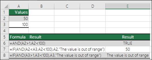
=AND(A2>1,A2 AND less than 100, otherwise it displays FALSE.

Displays the value in cell A2 if it’s less than A3 AND less than 100, otherwise it displays the message «The value is out of range».

=IF(AND(A3>1,A3 AND less than 100, otherwise it displays a message. You can substitute any message of your choice.

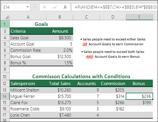
Here is a fairly common scenario where we need to calculate if sales people qualify for a bonus using IF and AND.

=$B$7,C14>=$B$5),B14*$B$8,0)» loading=»lazy»>

=IF(AND(B14>=$B$7,C14>=$B$5),B14*$B$8,0) – IF Total Sales are greater than or equal (>=) to the Sales Goal, AND Accounts are greater than or equal to (>=) the Account Goal, then multiply Total Sales by the Bonus %, otherwise return 0.

Need more help?

You can always ask an expert in the Excel Tech Community or get support in the Answers community.

Источник