
Explanation
In this example, the goal is to create a formula that will return «Done» in column E when a cell in column D contains a value. In other words, if the cell in column D is «not blank», then the formula should return «Done». In the worksheet shown, column D is is used to record the date a task was completed. Therefore, if the column contains a date (i.e. is not blank), we can assume the task is complete. This problem can be solved with the IF function alone or with the IF function and the ISBLANK function. It can also be solved with the LEN function. All three approaches are explained below.
IF function
The IF function runs a logical test and returns one value for a TRUE result, and another value for a FALSE result. You can use IF to test for a blank cell like this:
=IF(A1="",TRUE) // IF A1 is blank
=IF(A1<>"",TRUE) // IF A1 is not blank
In the first example, we test if A1 is empty with =»». In the second example, the <> symbol is a logical operator that means «not equal to», so the expression A1<>»» means A1 is «not empty». In the worksheet shown, we use the second idea in cell E5 like this:
=IF(D5<>"","Done","")
If D5 is «not empty», the result is «Done». If D5 is empty, IF returns an empty string («») which displays as nothing. As the formula is copied down, it returns «Done» only when a cell in column D contains a value. To display both «Done» and «Not done», you can adjust the formula like this:
=IF(D5<>"","Done","Not done")
ISBLANK function
Another way to solve this problem is with the ISBLANK function. The ISBLANK function returns TRUE when a cell is empty and FALSE if not. To use ISBLANK directly, you can rewrite the formula like this:
=IF(ISBLANK(D5),"","Done")
Notice the TRUE and FALSE results have been swapped. The logic now is if cell D5 is blank. To maintain the original logic, you can nest ISBLANK inside the NOT function like this:
=IF(NOT(ISBLANK(D5)),"Done","")
The NOT function simply reverses the result returned by ISBLANK.
LEN function
One problem with testing for blank cells in Excel is that ISBLANK(A1) or A1=»» will both return FALSE if A1 contains a formula that returns an empty string. In other words, if a formula returns an empty string in a cell, Excel interprets the cell as «not empty». To work around this problem, you can use the LEN function to test for characters in a cell like this:
=IF(LEN(A1)>0,TRUE)This is a much more literal formula. We are not asking Excel if A1 is blank, we are literally counting the characters in A1. The LEN function will return a positive number only when a cell contains actual characters.
Excel for Microsoft 365 Excel for Microsoft 365 for Mac Excel 2021 Excel 2021 for Mac Excel 2019 Excel 2019 for Mac Excel 2016 Excel 2016 for Mac Excel 2013 Excel 2010 Excel 2007 Excel for Mac 2011 More…Less
Sometimes you need to check if a cell is blank, generally because you might not want a formula to display a result without input.

In this case we’re using IF with the ISBLANK function:
-
=IF(ISBLANK(D2),»Blank»,»Not Blank»)
Which says IF(D2 is blank, then return «Blank», otherwise return «Not Blank»). You could just as easily use your own formula for the «Not Blank» condition as well. In the next example we’re using «» instead of ISBLANK. The «» essentially means «nothing».
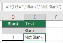
=IF(D3=»»,»Blank»,»Not Blank»)
This formula says IF(D3 is nothing, then return «Blank», otherwise «Not Blank»). Here is an example of a very common method of using «» to prevent a formula from calculating if a dependent cell is blank:
-
=IF(D3=»»,»»,YourFormula())
IF(D3 is nothing, then return nothing, otherwise calculate your formula).
Need more help?
Содержание
- Функция IsNull
- Синтаксис
- Замечания
- Пример
- См. также
- Поддержка и обратная связь
- Null in Excel
- Null in Excel
- ISBLANK Function to Find NULL Value in Excel
- #1 – How to Find NULL Cells in Excel?
- #2 – Shortcut Way of Finding NULL Cells in Excel
- #3 – How to Fill Our Values to NULL Cells in Excel?
- Things to Remember
- Recommended Articles
- Сравнение значений null в Power Query
- Blank and null values in Excel add-ins
- null input in 2-D Array
- null input for a property
- null property values in the response
- Blank input for a property
- VBA ISNULL
- VBA ISNULL Function
- How to Use VBA ISNULL Function in Excel?
- Example #1 – VBA ISNULL
- Pros of VBA IsNull
- Things to Remember
- Recommended Articles
Функция IsNull
Возвращает значение типа Boolean, которое указывает, не содержит ли выражение достоверных данных (Null).
Синтаксис
IsNull(выражение)
Замечания
IsNull возвращает значение True (Истина), если используется expression равное Null; в другом случае IsNull возвращает значение False (Ложь). Если expression состоит из нескольких переменных, значение Null, заданное для одной из них, приводит к возврату значения True для всего выражения.
Значение Null указывает, что Variant не содержит достоверных значений. Null не приравнивается к значению Empty (Пусто), которое указывает, что переменная не была инициализирована. Это также не то же самое, что строка нулевой длины («»), которую иногда называют пустой строкой.
Используйте функцию IsNull, чтобы определить, содержит ли выражение значение Null. Выражения, для которых может потребоваться значение True , в некоторых случаях, например If Var = Null и If Var <> Null , всегда имеют значение False. Это связано с тем, что любое выражение, содержащее значение NULL , само по себе имеет значение NULL и , следовательно, false.
Пример
В этом примере используется функция IsNull, чтобы определить, содержит ли переменная значение Null.
См. также
Поддержка и обратная связь
Есть вопросы или отзывы, касающиеся Office VBA или этой статьи? Руководство по другим способам получения поддержки и отправки отзывов см. в статье Поддержка Office VBA и обратная связь.
Источник
Null in Excel


Null is an error that occurs in Excel when the two or more cell references provided in a formula are incorrect, or the position they have been placed in is erroneous. For example, suppose we use space in formulas between two cell references; we will encounter a null error. In that case, there are two reasons to meet this error, one if we used an incorrect range reference and another when we use the intersect operator, which is the space character.
Null in Excel
NULL is nothing but nothing or blank in Excel. Usually, when working in Excel, we encounter many NULL or blank cells. We can use the formula and find out whether the particular cell is blank (NULL) or not.
We have several ways of finding the NULL cells in Excel. Today’s article will take a tour of dealing with NULL values in Excel.
How do you find which cell is blank or null? Yes, we must look at the particular cell and decide. Let us discover many methods of finding the null cells in Excel.
Table of contents
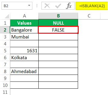
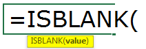
ISBLANK Function to Find NULL Value in Excel
![]()
The syntax is straightforward. Value is nothing but the cell reference; we are testing whether it is blank or not.
Note: ISBLANK will treat the single space as one character; if the cell has only space value, it will be recognized as a non-blank or non-null cell.
#1 – How to Find NULL Cells in Excel?
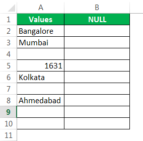
Assume we have the values below in the Excel file and want to test all the null cells in the range.
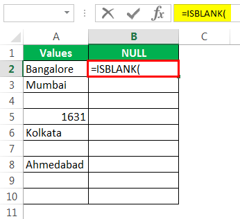
- Let us open the ISBLANK formula in cell B2 cell.
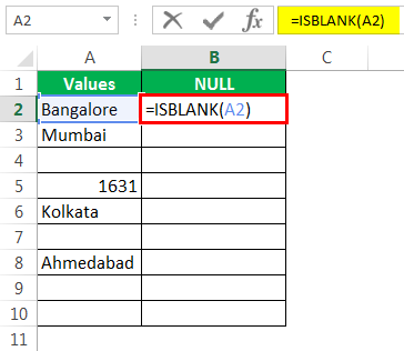
Select cell A2 as the argument. Since there is only one argument, close the bracket.
We got the result as given below:
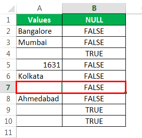
Then, drag and drop the formula to other remaining cells.

We got the results. But look at cell B7. Even though there is still no value in cell A7, the formula returned the result as a FALSE, non-null cell.
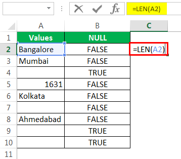
It counts the no. of characters and gives the result.

The LEN function returned the no. of character in the A7 cell as 1. So, there should be a character in it.
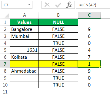
Let us edit the cell now. So, we found the space character here. Let us remove the space character to make the formula show accurate results.
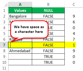
We have removed the space character, and the ISBLANK formula returned the result as TRUE. That is because even the LEN function says there are zero characters in cell A7.

#2 – Shortcut Way of Finding NULL Cells in Excel
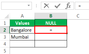
We have seen the traditional formula way to find the null cells. Without using the ISBLANK function, we can find the null cells.
Let us open the formula with an equal sign (=).
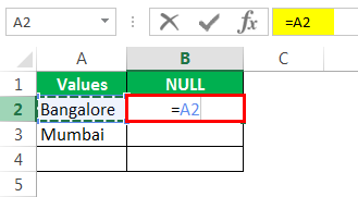
After the equal sign, select cell A2 as the reference.
Now open one more equal sign after the cell reference.
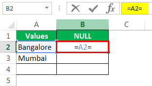
Now mention open double-quotes and close double-quotes. (“”)
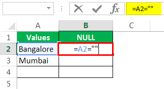
The sign double quotes (“”) says the selected cell is NULL or not. If the selected cell is NULL, we will get TRUE. Else, we will get FALSE.

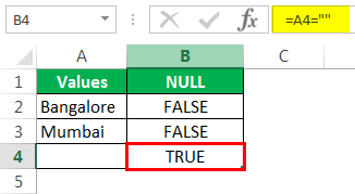
Drag the formula to the remaining cells.
We can see that in cell B7, we got the result as “TRUE.” So it means it is a null cell.
#3 – How to Fill Our Values to NULL Cells in Excel?
We have seen how to find the NULL cells in the Excel sheet. In our formula, we could only get TRUE or FALSE. But we can also receive our values for the NULL cells.
Consider the below data for an example.

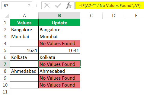
Step 1: Open the IF condition first.

Step 2: Here, we need to do a logical test. We need to test whether the cell is NULL or not. So apply A2=”.”
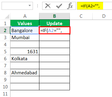
Step 3: If the logical test is TRUE (TRUE means cell is NULL), we need the result as “No Values Found.”
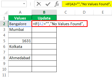
Step 4: If the logical test is FALSE (which means the cell contains values), then we need the same cell value.
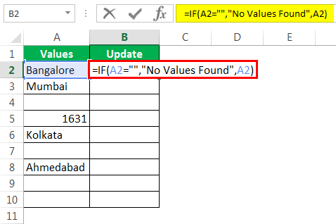
We got the result as the same cell value.
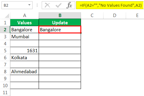
Step 5: Drag the formula to the remaining cells.
So, we have got our value of No Values Found for all the NULL cells.
Things to Remember
- Even space will be considered a character and treated as a non-empty cell.
- Instead of ISBLANK, we can also use double quotes (“ ”) to test the NULL cells.
- If the cell seems blank and the formula shows it as a non-null cell, then you need to test the number of characters using the LEN function.
Recommended Articles
This article is a guide to Null in Excel. We discuss the top methods to find null values in Excel using ISBLANK and shortcuts to replace those null cells, along with practical examples and a downloadable template. You may learn more about Excel from the following articles: –
Источник
Сравнение значений null в Power Query
Недавно мне нужно было сделать очень простую операцию в Power Query. В столбце с числами нужно было выполнить проверку “значение меньше N” и в новом столбце вывести соответствующий текст. Функция дополнительного столбца выглядит примерно так:
На самом деле некоторые значения – null (то есть пустые):
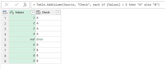
Данные содержат null и в результате сравнения возникает ошибка
И такая простая операция возвращает ошибку для этих значений!
Почему? Есть некоторая ловушка, спрятанная в глубинах документации (а именно на странице 67 PDF-файла “Power Query Formula Language Specification (October 2016)”, который можно найти тут.
Если коротко, то вот краткая выжимка из документации:
Значения null можно сравнивать на равенство, но null равен только null:
Но если вы хотите сравнить null с любым другим значением при помощи относительного оператора (например, , =), тогда результат сравнения будет не логическое значение типа true или false , а именно null . В разделе “6.7 Relational operators” об этом есть маленькое замечание:
If either or both operands are null , the result is the null value.
Так и в чем уловка? В выражении if…then…else после слова if должно идти логическое значение (например, как результат какого-то сравнения):
Когда мы сравниваем (практически любые) значения одного типа, мы в результате получаем логическое значение: true или false . Но в случае с null мы получим логическое значение только в случае, если мы сравниваем null на равенство:
НО если мы сделаем относительное сравнение null с SomeValue, тогда результат – НЕ логическое значение (он будет null ), и выражение if…then…else вернет ошибку:
Источник
Blank and null values in Excel add-ins
null and empty strings have special implications in the Excel JavaScript APIs. They’re used to represent empty cells, no formatting, or default values. This section details the use of null and empty string when getting and setting properties.
null input in 2-D Array
In Excel, a range is represented by a 2-D array, where the first dimension is rows and the second dimension is columns. To set values, number format, or formula for only specific cells within a range, specify the values, number format, or formula for those cells in the 2-D array, and specify null for all other cells in the 2-D array.
For example, to update the number format for only one cell within a range, and retain the existing number format for all other cells in the range, specify the new number format for the cell to update, and specify null for all other cells. The following code snippet sets a new number format for the fourth cell in the range, and leaves the number format unchanged for the first three cells in the range.
null input for a property
null is not a valid input for single property. For example, the following code snippet is not valid, as the values property of the range cannot be set to null .
Likewise, the following code snippet is not valid, as null is not a valid value for the color property.
null property values in the response
Formatting properties such as size and color will contain null values in the response when different values exist in the specified range. For example, if you retrieve a range and load its format.font.color property:
- If all cells in the range have the same font color, range.format.font.color specifies that color.
- If multiple font colors are present within the range, range.format.font.color is null .
Blank input for a property
When you specify a blank value for a property (i.e., two quotation marks with no space in-between » ), it will be interpreted as an instruction to clear or reset the property. For example:
- If you specify a blank value for the values property of a range, the content of the range is cleared.
- If you specify a blank value for the numberFormat property, the number format is reset to General .
- If you specify a blank value for the formula property and formulaLocale property, the formula values are cleared.
Источник
VBA ISNULL
VBA ISNULL Function
ISNULL function in VBA is used for finding the null value in excel. This seems easy but when we have a huge database which is connected to multiple files and sources and if we asked to find the Null in that, then any manual method will not work. For that, we have a function called IsNull in VBA which finds the Null value in any type of database or table. This can only be done in VBA, we do not have any such function in Excel.
Syntax of ISNULL in Excel VBA
Valuation, Hadoop, Excel, Mobile Apps, Web Development & many more.
The syntax for the VBA ISNULL function in excel is as follows:
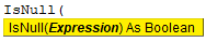
As we can see in the above screenshot, IsNull uses only one expression and to as Boolean. Which means it will give the answer as TRUE and FALSE values. If the data is Null then we will get TRUE or else we will get FALSE as output.
How to Use VBA ISNULL Function in Excel?
We will learn how to use a VBA ISNULL function with example in excel.
Example #1 – VBA ISNULL
Follow the below steps to use IsNull in Excel VBA.
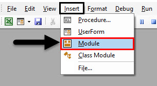
Step 1: To apply VBA IsNull, we need a module. For this go to the VBA window and under the Insert menu select Module as shown below.
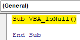
Step 2: Once we do that we will get a blank window of fresh Module. In that, write the subcategory of VBA IsNull or in any other name as per your need.
Code:
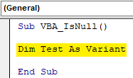
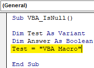
Step 3: For IsNull function, we will need one as a Variant. Where we can store any kind of value. Let’s have a first variable Test as Variant as shown below.
Code:
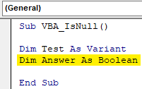
Step 4: As we know that IsNull works on Boolean. So we will need another variable. Let’s have our second variable Answer as Boolean as shown below. This will help us in knowing whether IsNull is TRUE or FALSE.
Code:
Step 5: Now give any value to the first variable Test. Let’s give it a text value “VBA Macro” as shown below.
Code:
Step 6: Now we will use our second variable Answer with IsNull function as shown below.
Code:
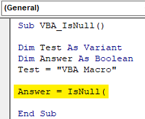
As we have seen in the explanation of VBA IsNull, that syntax of IsNull is Expression only. And this Expression can be a text, cell reference, direct value by entering manually or any other variable assigned to it.
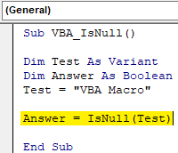
Step 7: We can enter anything in Expression. We have already assigned a text value to variable Test. Now select the variable into the expression.
Code:
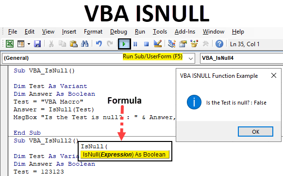
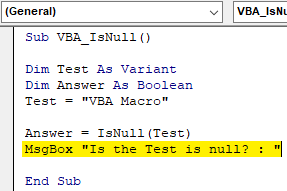
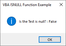
Step 8: Once done, then we will need a message box to print the value of IsNull if it is TRUE or FALSE. Insert Msgbox and give any statement which we want to see. Here we have considered “Is the Test is null?” as shown below.
Code:
Step 9: And then add rest of the variable which we defined above separated by the ampersand (&) as shown below which includes our second variable Answer and name of the message box as “VBA ISNULL Function Example”.
Code:
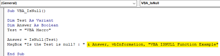
Step 10: Now compile the code by pressing F8 and run it by pressing the F5 key if there is no error found. We will see the Isnull function has returned the Answer as FALSE. Which means text “VBA Macro” is not null.
Step 11: Now we will see if numbers can be null or not. For this, we use a new module or we can use the same code that we have written above. In that, we just need to make changes. Assign any number to Test variable in place of text “VBA Macro”. Let’s consider that number as 123123 as shown below.
Code:
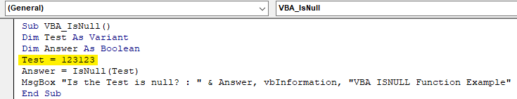
Step 12: Now again compile the code or we can compile the current step only by putting the cursor there and pressing F8 key. And run it. We will get the message box with the statement that our Test variable which is number 123123 is also not a Null. It is FALSE to call it a null.

Step 13: Now it is clear that neither Text nor Number can be Null. To test further, now we will consider a blank. A reference which has no value. For this, in the same previously written code put the double inverted (“”) commas with nothing in it in Test variable as shown below. Now we will is if a Blank can be a null or not.
Code:
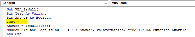
Step 14: We will get a message which says the Blank reference is also not null. It is FALSE to call it so.
Step 15: We have tried Text, Number and Blank for testing if they are null or not. Now we will text Null itself under variable Test as see if this is a null or not.
Code:
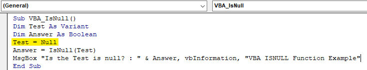
Step 16: Now run the code. We will in the message box the statement for “Is the Test is null?” has come TRUE.
Which means, in data if there are any cells with Blank, Space, Text or Number. Those cells will not be considered as Null.
Pros of VBA IsNull
- We can find if a cell is Null or not.
- We can test any variable if it is null or not.
- This quite helps in a big database which is fetched from some source.
Things to Remember
- IsNull finds only Null as Null. Text, Numbers, and Blanks are not null.
- IsNull is only applicable in VBA. Excel doesn’t have any function as IsNull or other matching function which can give the same result as IsNull.
- To use the code multiple times, it is better to save the excel in Macro Enable Excel format. This process helps in retaining the code for future use.
- IsNull only returns the value in the Boolean form, means in TRUE and FALSE
- Considering the Variant as Test variable allow us to use numbers, words and blank values in it. It considers all the type of values majorly used for Boolean.
Recommended Articles
This is a guide to VBA ISNULL. Here we discuss how to use Excel VBA ISNULL function along with practical examples and downloadable excel template. You can also go through our other suggested articles –
Источник
Null is an error that occurs in Excel when the two or more cell references provided in a formula are incorrect, or the position they have been placed in is erroneous. For example, suppose we use space in formulas between two cell references; we will encounter a null error. In that case, there are two reasons to meet this error, one if we used an incorrect range reference and another when we use the intersect operator, which is the space character.
NULL is nothing but nothing or blank in Excel. Usually, when working in Excel, we encounter many NULL or blank cells. We can use the formula and find out whether the particular cell is blank (NULL) or not.
We have several ways of finding the NULL cells in Excel. Today’s article will take a tour of dealing with NULL values in Excel.
How do you find which cell is blank or null? Yes, we must look at the particular cell and decide. Let us discover many methods of finding the null cells in Excel.
Table of contents
- Null in Excel
- ISBLANK Function to Find NULL Value in Excel
- #1 – How to Find NULL Cells in Excel?
- #2 – Shortcut Way of Finding NULL Cells in Excel
- #3 – How to Fill Our Own Values to NULL Cells in Excel?
- Things to Remember
- Recommended Articles
ISBLANK Function to Find NULL Value in Excel
In Excel, we have an ISBLANK function, which can find the blank cells in the worksheet. First, let us look at the syntax of the ISBLANK functionISBLANK in Excel is a logical function that checks if a target cell is blank or not. It returns the output “true” if the cell is empty (blank) or “false” if the cell is not empty. It is also known as referencing worksheet function and is grouped under the information function of Excel
read more.
The syntax is straightforward. Value is nothing but the cell reference; we are testing whether it is blank or not.
Since ISBLANK is a logical excel functionA logical test in Excel results in an analytical output, either true or false. The equals to operator, “=,” is the most commonly used logical test.read more, it will either return TRUE or FALSE. If the cell is NULL, it will return TRUE, or else it will return FALSE.
Note: ISBLANK will treat the single space as one character; if the cell has only space value, it will be recognized as a non-blank or non-null cell.
#1 – How to Find NULL Cells in Excel?
You can download this Null Value Excel Template here – Null Value Excel Template
Assume we have the values below in the Excel file and want to test all the null cells in the range.
- Let us open the ISBLANK formula in cell B2 cell.

- Select cell A2 as the argument. Since there is only one argument, close the bracket.

- We got the result as given below:

- Then, drag and drop the formula to other remaining cells.

- We got the results. But look at cell B7. Even though there is still no value in cell A7, the formula returned the result as a FALSE, non-null cell.

- Let us apply the LEN function in excelThe Len function returns the length of a given string. It calculates the number of characters in a given string as input. It is a text function in Excel as well as an inbuilt function that can be accessed by typing =LEN( and entering a string as input.read more to find the number of characters in the cell.

- It counts the no. of characters and gives the result.

- The LEN function returned the no. of character in the A7 cell as 1. So, there should be a character in it.

- Let us edit the cell now. So, we found the space character here. Let us remove the space character to make the formula show accurate results.

- We have removed the space character, and the ISBLANK formula returned the result as TRUE. That is because even the LEN function says there are zero characters in cell A7.

#2 – Shortcut Way of Finding NULL Cells in Excel
We have seen the traditional formula way to find the null cells. Without using the ISBLANK function, we can find the null cells.
Let us open the formula with an equal sign (=).
After the equal sign, select cell A2 as the reference.
Now open one more equal sign after the cell reference.
Now mention open double-quotes and close double-quotes. (“”)
The sign double quotes (“”) says the selected cell is NULL or not. If the selected cell is NULL, we will get TRUE. Else, we will get FALSE.
Drag the formula to the remaining cells.
We can see that in cell B7, we got the result as “TRUE.” So it means it is a null cell.
#3 – How to Fill Our Values to NULL Cells in Excel?
We have seen how to find the NULL cells in the Excel sheet. In our formula, we could only get TRUE or FALSE. But we can also receive our values for the NULL cells.
Consider the below data for an example.
Step 1: Open the IF condition first.
Step 2: Here, we need to do a logical test. We need to test whether the cell is NULL or not. So apply A2=”.”
Step 3: If the logical test is TRUE (TRUE means cell is NULL), we need the result as “No Values Found.”
Step 4: If the logical test is FALSE (which means the cell contains values), then we need the same cell value.
We got the result as the same cell value.
Step 5: Drag the formula to the remaining cells.
So, we have got our value of No Values Found for all the NULL cells.
Things to Remember
- Even space will be considered a character and treated as a non-empty cell.
- Instead of ISBLANK, we can also use double quotes (“ ”) to test the NULL cells.
- If the cell seems blank and the formula shows it as a non-null cell, then you need to test the number of characters using the LEN function.
Recommended Articles
This article is a guide to Null in Excel. We discuss the top methods to find null values in Excel using ISBLANK and shortcuts to replace those null cells, along with practical examples and a downloadable template. You may learn more about Excel from the following articles: –
- Excel Count RowsThere are numerous ways to count rows in Excel using the appropriate formula, whether they are data rows, empty rows, or rows containing numerical/text values. Depending on the circumstance, you can use the COUNTA, COUNT, COUNTBLANK, or COUNTIF functions.read more
- VBA RangeRange is a property in VBA that helps specify a particular cell, a range of cells, a row, a column, or a three-dimensional range. In the context of the Excel worksheet, the VBA range object includes a single cell or multiple cells spread across various rows and columns.read more
- Countif not Blank in Excel
- Remove Blank Rows in ExcelThere are several methods for deleting blank rows from Excel: 1) Manually deleting blank rows if there are few blank rows 2) Use the formula delete 3) Use the filter to find and delete blank rows.read more
-
#2
Try
=IF(AND(E99<>»»,OR(E99=»No»,I99<=4,E99=»text»,I99=»text»)),1,0)
-
#3
Sorry, for clarification: I also do not want null values in col I. I tried the following, but I am not getting the right answer:
=IF(AND((E99<>»»),OR (I99<>»»),,OR(E99=»No»,I99<=4,E99=»text»,I99=»text»)),1,0)
-
#4
=IF(AND((E99<>»»),OR (I99<>»»),OR(E99=»No»,I99<=4,E99=»text»,I99=»text»)),1,0)
Correction without extra comma
-
#5
Try
=IF(AND(E99<>»»,I99<>»»,OR(E99=»No»,I99<=4,E99=»text»,I99=»text»)),1,0)
-
#6
It did not work. I may not have explained it correctly. Col E contains Yes, No and blanks, Col I contains numbers 1-10 and blanks. I want to bring back: Col E = No OR Col I <=4, no blanks
<TABLE style=»WIDTH: 288pt; BORDER-COLLAPSE: collapse» border=0 cellSpacing=0 cellPadding=0 width=384><COLGROUP><COL style=»WIDTH: 48pt» span=6 width=64><TBODY><TR style=»HEIGHT: 33.75pt» height=45><TD style=»BORDER-BOTTOM: windowtext 0.5pt solid; BORDER-LEFT: windowtext 0.5pt solid; BACKGROUND-COLOR: #4bacc6; WIDTH: 48pt; HEIGHT: 33.75pt; BORDER-TOP: windowtext 0.5pt solid; BORDER-RIGHT: windowtext 0.5pt solid» class=xl63 height=45 width=64>Geo</TD><TD style=»BORDER-BOTTOM: windowtext 0.5pt solid; BORDER-LEFT: windowtext; BACKGROUND-COLOR: #4bacc6; WIDTH: 48pt; BORDER-TOP: windowtext 0.5pt solid; BORDER-RIGHT: windowtext 0.5pt solid» id=td_post_2824097 class=xl63 width=64>Region</TD><TD style=»BORDER-BOTTOM: windowtext 0.5pt solid; BORDER-LEFT: windowtext; BACKGROUND-COLOR: #4bacc6; WIDTH: 48pt; BORDER-TOP: windowtext 0.5pt solid; BORDER-RIGHT: windowtext 0.5pt solid» class=xl63 width=64>Rep</TD><TD style=»BORDER-BOTTOM: windowtext 0.5pt solid; BORDER-LEFT: windowtext; BACKGROUND-COLOR: #4bacc6; WIDTH: 48pt; BORDER-TOP: windowtext 0.5pt solid; BORDER-RIGHT: windowtext 0.5pt solid» class=xl63 width=64>Cust#</TD><TD style=»BORDER-BOTTOM: windowtext 0.5pt solid; BORDER-LEFT: windowtext; BACKGROUND-COLOR: #4bacc6; WIDTH: 48pt; BORDER-TOP: windowtext 0.5pt solid; BORDER-RIGHT: windowtext 0.5pt solid» class=xl63 width=64>Was the Issue Addressed?</TD><TD style=»BORDER-BOTTOM: windowtext 0.5pt solid; BORDER-LEFT: windowtext; BACKGROUND-COLOR: #4bacc6; WIDTH: 48pt; BORDER-TOP: windowtext 0.5pt solid; BORDER-RIGHT: windowtext 0.5pt solid» class=xl63 width=64>Level of Support</TD></TR><TR style=»HEIGHT: 15pt» height=20><TD style=»BORDER-BOTTOM: windowtext 0.5pt solid; BORDER-LEFT: windowtext 0.5pt solid; BACKGROUND-COLOR: transparent; WIDTH: 48pt; HEIGHT: 15pt; BORDER-TOP: windowtext; BORDER-RIGHT: windowtext 0.5pt solid» class=xl64 height=20 width=64>Americas1</TD><TD style=»BORDER-BOTTOM: windowtext 0.5pt solid; BORDER-LEFT: windowtext; BACKGROUND-COLOR: transparent; WIDTH: 48pt; BORDER-TOP: windowtext; BORDER-RIGHT: windowtext 0.5pt solid» class=xl64 width=64>East</TD><TD style=»BORDER-BOTTOM: windowtext 0.5pt solid; BORDER-LEFT: windowtext; BACKGROUND-COLOR: transparent; WIDTH: 48pt; BORDER-TOP: windowtext; BORDER-RIGHT: windowtext 0.5pt solid» class=xl64 width=64>Rep1</TD><TD style=»BORDER-BOTTOM: windowtext 0.5pt solid; BORDER-LEFT: windowtext; BACKGROUND-COLOR: transparent; WIDTH: 48pt; BORDER-TOP: windowtext; BORDER-RIGHT: windowtext 0.5pt solid» class=xl64 width=64>70706230</TD><TD style=»BORDER-BOTTOM: windowtext 0.5pt solid; BORDER-LEFT: windowtext; BACKGROUND-COLOR: transparent; WIDTH: 48pt; BORDER-TOP: windowtext; BORDER-RIGHT: windowtext 0.5pt solid» class=xl64 width=64>Yes</TD><TD style=»BORDER-BOTTOM: windowtext 0.5pt solid; BORDER-LEFT: windowtext; BACKGROUND-COLOR: transparent; WIDTH: 48pt; BORDER-TOP: windowtext; BORDER-RIGHT: windowtext 0.5pt solid» class=xl64 width=64> </TD></TR><TR style=»HEIGHT: 15pt» height=20><TD style=»BORDER-BOTTOM: windowtext 0.5pt solid; BORDER-LEFT: windowtext 0.5pt solid; BACKGROUND-COLOR: transparent; WIDTH: 48pt; HEIGHT: 15pt; BORDER-TOP: windowtext; BORDER-RIGHT: windowtext 0.5pt solid» class=xl64 height=20 width=64>Americas2</TD><TD style=»BORDER-BOTTOM: windowtext 0.5pt solid; BORDER-LEFT: windowtext; BACKGROUND-COLOR: transparent; WIDTH: 48pt; BORDER-TOP: windowtext; BORDER-RIGHT: windowtext 0.5pt solid» class=xl64 width=64>West</TD><TD style=»BORDER-BOTTOM: windowtext 0.5pt solid; BORDER-LEFT: windowtext; BACKGROUND-COLOR: transparent; WIDTH: 48pt; BORDER-TOP: windowtext; BORDER-RIGHT: windowtext 0.5pt solid» class=xl64 width=64>Rep2</TD><TD style=»BORDER-BOTTOM: windowtext 0.5pt solid; BORDER-LEFT: windowtext; BACKGROUND-COLOR: transparent; WIDTH: 48pt; BORDER-TOP: windowtext; BORDER-RIGHT: windowtext 0.5pt solid» class=xl64 width=64>70723549</TD><TD style=»BORDER-BOTTOM: windowtext 0.5pt solid; BORDER-LEFT: windowtext; BACKGROUND-COLOR: transparent; WIDTH: 48pt; BORDER-TOP: windowtext; BORDER-RIGHT: windowtext 0.5pt solid» class=xl64 width=64> </TD><TD style=»BORDER-BOTTOM: windowtext 0.5pt solid; BORDER-LEFT: windowtext; BACKGROUND-COLOR: transparent; WIDTH: 48pt; BORDER-TOP: windowtext; BORDER-RIGHT: windowtext 0.5pt solid» class=xl64 width=64>10</TD></TR><TR style=»HEIGHT: 15pt» height=20><TD style=»BORDER-BOTTOM: windowtext 0.5pt solid; BORDER-LEFT: windowtext 0.5pt solid; BACKGROUND-COLOR: transparent; WIDTH: 48pt; HEIGHT: 15pt; BORDER-TOP: windowtext; BORDER-RIGHT: windowtext 0.5pt solid» class=xl64 height=20 width=64>EMEA</TD><TD style=»BORDER-BOTTOM: windowtext 0.5pt solid; BORDER-LEFT: windowtext; BACKGROUND-COLOR: transparent; WIDTH: 48pt; BORDER-TOP: windowtext; BORDER-RIGHT: windowtext 0.5pt solid» class=xl64 width=64>North </TD><TD style=»BORDER-BOTTOM: windowtext 0.5pt solid; BORDER-LEFT: windowtext; BACKGROUND-COLOR: transparent; WIDTH: 48pt; BORDER-TOP: windowtext; BORDER-RIGHT: windowtext 0.5pt solid» class=xl64 width=64>Rep3</TD><TD style=»BORDER-BOTTOM: windowtext 0.5pt solid; BORDER-LEFT: windowtext; BACKGROUND-COLOR: transparent; WIDTH: 48pt; BORDER-TOP: windowtext; BORDER-RIGHT: windowtext 0.5pt solid» class=xl64 width=64>60696810</TD><TD style=»BORDER-BOTTOM: windowtext 0.5pt solid; BORDER-LEFT: windowtext; BACKGROUND-COLOR: transparent; WIDTH: 48pt; BORDER-TOP: windowtext; BORDER-RIGHT: windowtext 0.5pt solid» class=xl64 width=64>Yes</TD><TD style=»BORDER-BOTTOM: windowtext 0.5pt solid; BORDER-LEFT: windowtext; BACKGROUND-COLOR: transparent; WIDTH: 48pt; BORDER-TOP: windowtext; BORDER-RIGHT: windowtext 0.5pt solid» class=xl64 width=64> </TD></TR><TR style=»HEIGHT: 15pt» height=20><TD style=»BORDER-BOTTOM: windowtext 0.5pt solid; BORDER-LEFT: windowtext 0.5pt solid; BACKGROUND-COLOR: transparent; WIDTH: 48pt; HEIGHT: 15pt; BORDER-TOP: windowtext; BORDER-RIGHT: windowtext 0.5pt solid» class=xl64 height=20 width=64>Ap</TD><TD style=»BORDER-BOTTOM: windowtext 0.5pt solid; BORDER-LEFT: windowtext; BACKGROUND-COLOR: transparent; WIDTH: 48pt; BORDER-TOP: windowtext; BORDER-RIGHT: windowtext 0.5pt solid» class=xl64 width=64>South</TD><TD style=»BORDER-BOTTOM: windowtext 0.5pt solid; BORDER-LEFT: windowtext; BACKGROUND-COLOR: transparent; WIDTH: 48pt; BORDER-TOP: windowtext; BORDER-RIGHT: windowtext 0.5pt solid» class=xl64 width=64>Rep5</TD><TD style=»BORDER-BOTTOM: windowtext 0.5pt solid; BORDER-LEFT: windowtext; BACKGROUND-COLOR: transparent; WIDTH: 48pt; BORDER-TOP: windowtext; BORDER-RIGHT: windowtext 0.5pt solid» class=xl64 width=64>90719603</TD><TD style=»BORDER-BOTTOM: windowtext 0.5pt solid; BORDER-LEFT: windowtext; BACKGROUND-COLOR: transparent; WIDTH: 48pt; BORDER-TOP: windowtext; BORDER-RIGHT: windowtext 0.5pt solid» class=xl64 width=64>No</TD><TD style=»BORDER-BOTTOM: windowtext 0.5pt solid; BORDER-LEFT: windowtext; BACKGROUND-COLOR: transparent; WIDTH: 48pt; BORDER-TOP: windowtext; BORDER-RIGHT: windowtext 0.5pt solid» class=xl64 width=64>3</TD></TR><TR style=»HEIGHT: 15pt» height=20><TD style=»BORDER-BOTTOM: windowtext 0.5pt solid; BORDER-LEFT: windowtext 0.5pt solid; BACKGROUND-COLOR: transparent; WIDTH: 48pt; HEIGHT: 15pt; BORDER-TOP: windowtext; BORDER-RIGHT: windowtext 0.5pt solid» class=xl64 height=20 width=64>Japan</TD><TD style=»BORDER-BOTTOM: windowtext 0.5pt solid; BORDER-LEFT: windowtext; BACKGROUND-COLOR: transparent; WIDTH: 48pt; BORDER-TOP: windowtext; BORDER-RIGHT: windowtext 0.5pt solid» class=xl64 width=64>South</TD><TD style=»BORDER-BOTTOM: windowtext 0.5pt solid; BORDER-LEFT: windowtext; BACKGROUND-COLOR: transparent; WIDTH: 48pt; BORDER-TOP: windowtext; BORDER-RIGHT: windowtext 0.5pt solid» class=xl64 width=64>Rep7</TD><TD style=»BORDER-BOTTOM: windowtext 0.5pt solid; BORDER-LEFT: windowtext; BACKGROUND-COLOR: transparent; WIDTH: 48pt; BORDER-TOP: windowtext; BORDER-RIGHT: windowtext 0.5pt solid» class=xl64 width=64>80713298</TD><TD style=»BORDER-BOTTOM: windowtext 0.5pt solid; BORDER-LEFT: windowtext; BACKGROUND-COLOR: transparent; WIDTH: 48pt; BORDER-TOP: windowtext; BORDER-RIGHT: windowtext 0.5pt solid» class=xl64 width=64>Yes</TD><TD style=»BORDER-BOTTOM: windowtext 0.5pt solid; BORDER-LEFT: windowtext; BACKGROUND-COLOR: transparent; WIDTH: 48pt; BORDER-TOP: windowtext; BORDER-RIGHT: windowtext 0.5pt solid» class=xl64 width=64>8</TD></TR><TR style=»HEIGHT: 15pt» height=20><TD style=»BORDER-BOTTOM: windowtext 0.5pt solid; BORDER-LEFT: windowtext 0.5pt solid; BACKGROUND-COLOR: transparent; WIDTH: 48pt; HEIGHT: 15pt; BORDER-TOP: windowtext; BORDER-RIGHT: windowtext 0.5pt solid» class=xl64 height=20 width=64>EMEA</TD><TD style=»BORDER-BOTTOM: windowtext 0.5pt solid; BORDER-LEFT: windowtext; BACKGROUND-COLOR: transparent; WIDTH: 48pt; BORDER-TOP: windowtext; BORDER-RIGHT: windowtext 0.5pt solid» class=xl64 width=64>East</TD><TD style=»BORDER-BOTTOM: windowtext 0.5pt solid; BORDER-LEFT: windowtext; BACKGROUND-COLOR: transparent; WIDTH: 48pt; BORDER-TOP: windowtext; BORDER-RIGHT: windowtext 0.5pt solid» class=xl64 width=64>Rep8</TD><TD style=»BORDER-BOTTOM: windowtext 0.5pt solid; BORDER-LEFT: windowtext; BACKGROUND-COLOR: transparent; WIDTH: 48pt; BORDER-TOP: windowtext; BORDER-RIGHT: windowtext 0.5pt solid» class=xl64 width=64>20716087</TD><TD style=»BORDER-BOTTOM: windowtext 0.5pt solid; BORDER-LEFT: windowtext; BACKGROUND-COLOR: transparent; WIDTH: 48pt; BORDER-TOP: windowtext; BORDER-RIGHT: windowtext 0.5pt solid» class=xl64 width=64>Yes</TD><TD style=»BORDER-BOTTOM: windowtext 0.5pt solid; BORDER-LEFT: windowtext; BACKGROUND-COLOR: transparent; WIDTH: 48pt; BORDER-TOP: windowtext; BORDER-RIGHT: windowtext 0.5pt solid» class=xl64 width=64>4</TD></TR><TR style=»HEIGHT: 15pt» height=20><TD style=»BORDER-BOTTOM: windowtext 0.5pt solid; BORDER-LEFT: windowtext 0.5pt solid; BACKGROUND-COLOR: transparent; WIDTH: 48pt; HEIGHT: 15pt; BORDER-TOP: windowtext; BORDER-RIGHT: windowtext 0.5pt solid» class=xl64 height=20 width=64>EMEA</TD><TD style=»BORDER-BOTTOM: windowtext 0.5pt solid; BORDER-LEFT: windowtext; BACKGROUND-COLOR: transparent; WIDTH: 48pt; BORDER-TOP: windowtext; BORDER-RIGHT: windowtext 0.5pt solid» class=xl64 width=64>East</TD><TD style=»BORDER-BOTTOM: windowtext 0.5pt solid; BORDER-LEFT: windowtext; BACKGROUND-COLOR: transparent; WIDTH: 48pt; BORDER-TOP: windowtext; BORDER-RIGHT: windowtext 0.5pt solid» class=xl64 width=64>Rep9</TD><TD style=»BORDER-BOTTOM: windowtext 0.5pt solid; BORDER-LEFT: windowtext; BACKGROUND-COLOR: transparent; WIDTH: 48pt; BORDER-TOP: windowtext; BORDER-RIGHT: windowtext 0.5pt solid» class=xl64 width=64>20716088</TD><TD style=»BORDER-BOTTOM: windowtext 0.5pt solid; BORDER-LEFT: windowtext; BACKGROUND-COLOR: transparent; WIDTH: 48pt; BORDER-TOP: windowtext; BORDER-RIGHT: windowtext 0.5pt solid» class=xl64 width=64> </TD><TD style=»BORDER-BOTTOM: windowtext 0.5pt solid; BORDER-LEFT: windowtext; BACKGROUND-COLOR: transparent; WIDTH: 48pt; BORDER-TOP: windowtext; BORDER-RIGHT: windowtext 0.5pt solid» class=xl64 width=64> </TD></TR><TR style=»HEIGHT: 15pt» height=20><TD style=»BORDER-BOTTOM: windowtext 0.5pt solid; BORDER-LEFT: windowtext 0.5pt solid; BACKGROUND-COLOR: transparent; WIDTH: 48pt; HEIGHT: 15pt; BORDER-TOP: windowtext; BORDER-RIGHT: windowtext 0.5pt solid» class=xl64 height=20 width=64>EMEA</TD><TD style=»BORDER-BOTTOM: windowtext 0.5pt solid; BORDER-LEFT: windowtext; BACKGROUND-COLOR: transparent; WIDTH: 48pt; BORDER-TOP: windowtext; BORDER-RIGHT: windowtext 0.5pt solid» class=xl64 width=64>East</TD><TD style=»BORDER-BOTTOM: windowtext 0.5pt solid; BORDER-LEFT: windowtext; BACKGROUND-COLOR: transparent; WIDTH: 48pt; BORDER-TOP: windowtext; BORDER-RIGHT: windowtext 0.5pt solid» class=xl64 width=64>Rep10</TD><TD style=»BORDER-BOTTOM: windowtext 0.5pt solid; BORDER-LEFT: windowtext; BACKGROUND-COLOR: transparent; WIDTH: 48pt; BORDER-TOP: windowtext; BORDER-RIGHT: windowtext 0.5pt solid» class=xl64 width=64>20716089</TD><TD style=»BORDER-BOTTOM: windowtext 0.5pt solid; BORDER-LEFT: windowtext; BACKGROUND-COLOR: transparent; WIDTH: 48pt; BORDER-TOP: windowtext; BORDER-RIGHT: windowtext 0.5pt solid» class=xl64 width=64>No</TD><TD style=»BORDER-BOTTOM: windowtext 0.5pt solid; BORDER-LEFT: windowtext; BACKGROUND-COLOR: transparent; WIDTH: 48pt; BORDER-TOP: windowtext; BORDER-RIGHT: windowtext 0.5pt solid» class=xl64 width=64>2</TD></TR><TR style=»HEIGHT: 15pt» height=20><TD style=»BORDER-BOTTOM: windowtext 0.5pt solid; BORDER-LEFT: windowtext 0.5pt solid; BACKGROUND-COLOR: transparent; WIDTH: 48pt; HEIGHT: 15pt; BORDER-TOP: windowtext; BORDER-RIGHT: windowtext 0.5pt solid» class=xl64 height=20 width=64>EMEA</TD><TD style=»BORDER-BOTTOM: windowtext 0.5pt solid; BORDER-LEFT: windowtext; BACKGROUND-COLOR: transparent; WIDTH: 48pt; BORDER-TOP: windowtext; BORDER-RIGHT: windowtext 0.5pt solid» class=xl64 width=64>East</TD><TD style=»BORDER-BOTTOM: windowtext 0.5pt solid; BORDER-LEFT: windowtext; BACKGROUND-COLOR: transparent; WIDTH: 48pt; BORDER-TOP: windowtext; BORDER-RIGHT: windowtext 0.5pt solid» class=xl64 width=64>Rep11</TD><TD style=»BORDER-BOTTOM: windowtext 0.5pt solid; BORDER-LEFT: windowtext; BACKGROUND-COLOR: transparent; WIDTH: 48pt; BORDER-TOP: windowtext; BORDER-RIGHT: windowtext 0.5pt solid» class=xl64 width=64>20716090</TD><TD style=»BORDER-BOTTOM: windowtext 0.5pt solid; BORDER-LEFT: windowtext; BACKGROUND-COLOR: transparent; WIDTH: 48pt; BORDER-TOP: windowtext; BORDER-RIGHT: windowtext 0.5pt solid» class=xl64 width=64>Yes</TD><TD style=»BORDER-BOTTOM: windowtext 0.5pt solid; BORDER-LEFT: windowtext; BACKGROUND-COLOR: transparent; WIDTH: 48pt; BORDER-TOP: windowtext; BORDER-RIGHT: windowtext 0.5pt solid» class=xl64 width=64>1</TD></TR></TBODY></TABLE>
=IF(AND(E693<>»», I693<>»»,OR(E693=»No»,I693<=4,E693=»text»,I693=»text»)),1,»») is not working
-
#7
Hi,
If anyone has a suggestion, it would be appreciated.
It did not work. I may not have explained it correctly. Col E contains Yes, No and blanks, Col I contains numbers 1-10 and blanks. I want to bring back: Col E = No OR Col I <=4, no blanks
<TABLE style=»WIDTH: 288pt; BORDER-COLLAPSE: collapse» border=0 cellSpacing=0 cellPadding=0 width=384><COLGROUP><COL style=»WIDTH: 48pt» span=6 width=64><TBODY><TR style=»HEIGHT: 33.75pt» height=45><TD style=»BORDER-BOTTOM: windowtext 0.5pt solid; BORDER-LEFT: windowtext 0.5pt solid; BACKGROUND-COLOR: #4bacc6; WIDTH: 48pt; HEIGHT: 33.75pt; BORDER-TOP: windowtext 0.5pt solid; BORDER-RIGHT: windowtext 0.5pt solid» class=xl63 height=45 width=64>Geo</TD><TD style=»BORDER-BOTTOM: windowtext 0.5pt solid; BACKGROUND-COLOR: #4bacc6; WIDTH: 48pt; BORDER-LEFT-COLOR: windowtext; BORDER-TOP: windowtext 0.5pt solid; BORDER-RIGHT: windowtext 0.5pt solid» id=td_post_2824097 class=xl63 width=64>Region</TD><TD style=»BORDER-BOTTOM: windowtext 0.5pt solid; BACKGROUND-COLOR: #4bacc6; WIDTH: 48pt; BORDER-LEFT-COLOR: windowtext; BORDER-TOP: windowtext 0.5pt solid; BORDER-RIGHT: windowtext 0.5pt solid» class=xl63 width=64>Rep</TD><TD style=»BORDER-BOTTOM: windowtext 0.5pt solid; BACKGROUND-COLOR: #4bacc6; WIDTH: 48pt; BORDER-LEFT-COLOR: windowtext; BORDER-TOP: windowtext 0.5pt solid; BORDER-RIGHT: windowtext 0.5pt solid» class=xl63 width=64>Cust#</TD><TD style=»BORDER-BOTTOM: windowtext 0.5pt solid; BACKGROUND-COLOR: #4bacc6; WIDTH: 48pt; BORDER-LEFT-COLOR: windowtext; BORDER-TOP: windowtext 0.5pt solid; BORDER-RIGHT: windowtext 0.5pt solid» class=xl63 width=64>Was the Issue Addressed?</TD><TD style=»BORDER-BOTTOM: windowtext 0.5pt solid; BACKGROUND-COLOR: #4bacc6; WIDTH: 48pt; BORDER-LEFT-COLOR: windowtext; BORDER-TOP: windowtext 0.5pt solid; BORDER-RIGHT: windowtext 0.5pt solid» class=xl63 width=64>Level of Support</TD></TR><TR style=»HEIGHT: 15pt» height=20><TD style=»BORDER-BOTTOM: windowtext 0.5pt solid; BORDER-LEFT: windowtext 0.5pt solid; BACKGROUND-COLOR: transparent; BORDER-TOP-COLOR: windowtext; WIDTH: 48pt; HEIGHT: 15pt; BORDER-RIGHT: windowtext 0.5pt solid» class=xl64 height=20 width=64>Americas1</TD><TD style=»BORDER-BOTTOM: windowtext 0.5pt solid; BACKGROUND-COLOR: transparent; BORDER-TOP-COLOR: windowtext; WIDTH: 48pt; BORDER-LEFT-COLOR: windowtext; BORDER-RIGHT: windowtext 0.5pt solid» class=xl64 width=64>East</TD><TD style=»BORDER-BOTTOM: windowtext 0.5pt solid; BACKGROUND-COLOR: transparent; BORDER-TOP-COLOR: windowtext; WIDTH: 48pt; BORDER-LEFT-COLOR: windowtext; BORDER-RIGHT: windowtext 0.5pt solid» class=xl64 width=64>Rep1</TD><TD style=»BORDER-BOTTOM: windowtext 0.5pt solid; BACKGROUND-COLOR: transparent; BORDER-TOP-COLOR: windowtext; WIDTH: 48pt; BORDER-LEFT-COLOR: windowtext; BORDER-RIGHT: windowtext 0.5pt solid» class=xl64 width=64>70706230</TD><TD style=»BORDER-BOTTOM: windowtext 0.5pt solid; BACKGROUND-COLOR: transparent; BORDER-TOP-COLOR: windowtext; WIDTH: 48pt; BORDER-LEFT-COLOR: windowtext; BORDER-RIGHT: windowtext 0.5pt solid» class=xl64 width=64>Yes</TD><TD style=»BORDER-BOTTOM: windowtext 0.5pt solid; BACKGROUND-COLOR: transparent; BORDER-TOP-COLOR: windowtext; WIDTH: 48pt; BORDER-LEFT-COLOR: windowtext; BORDER-RIGHT: windowtext 0.5pt solid» class=xl64 width=64></TD></TR><TR style=»HEIGHT: 15pt» height=20><TD style=»BORDER-BOTTOM: windowtext 0.5pt solid; BORDER-LEFT: windowtext 0.5pt solid; BACKGROUND-COLOR: transparent; BORDER-TOP-COLOR: windowtext; WIDTH: 48pt; HEIGHT: 15pt; BORDER-RIGHT: windowtext 0.5pt solid» class=xl64 height=20 width=64>Americas2</TD><TD style=»BORDER-BOTTOM: windowtext 0.5pt solid; BACKGROUND-COLOR: transparent; BORDER-TOP-COLOR: windowtext; WIDTH: 48pt; BORDER-LEFT-COLOR: windowtext; BORDER-RIGHT: windowtext 0.5pt solid» class=xl64 width=64>West</TD><TD style=»BORDER-BOTTOM: windowtext 0.5pt solid; BACKGROUND-COLOR: transparent; BORDER-TOP-COLOR: windowtext; WIDTH: 48pt; BORDER-LEFT-COLOR: windowtext; BORDER-RIGHT: windowtext 0.5pt solid» class=xl64 width=64>Rep2</TD><TD style=»BORDER-BOTTOM: windowtext 0.5pt solid; BACKGROUND-COLOR: transparent; BORDER-TOP-COLOR: windowtext; WIDTH: 48pt; BORDER-LEFT-COLOR: windowtext; BORDER-RIGHT: windowtext 0.5pt solid» class=xl64 width=64>70723549</TD><TD style=»BORDER-BOTTOM: windowtext 0.5pt solid; BACKGROUND-COLOR: transparent; BORDER-TOP-COLOR: windowtext; WIDTH: 48pt; BORDER-LEFT-COLOR: windowtext; BORDER-RIGHT: windowtext 0.5pt solid» class=xl64 width=64></TD><TD style=»BORDER-BOTTOM: windowtext 0.5pt solid; BACKGROUND-COLOR: transparent; BORDER-TOP-COLOR: windowtext; WIDTH: 48pt; BORDER-LEFT-COLOR: windowtext; BORDER-RIGHT: windowtext 0.5pt solid» class=xl64 width=64>10</TD></TR><TR style=»HEIGHT: 15pt» height=20><TD style=»BORDER-BOTTOM: windowtext 0.5pt solid; BORDER-LEFT: windowtext 0.5pt solid; BACKGROUND-COLOR: transparent; BORDER-TOP-COLOR: windowtext; WIDTH: 48pt; HEIGHT: 15pt; BORDER-RIGHT: windowtext 0.5pt solid» class=xl64 height=20 width=64>EMEA</TD><TD style=»BORDER-BOTTOM: windowtext 0.5pt solid; BACKGROUND-COLOR: transparent; BORDER-TOP-COLOR: windowtext; WIDTH: 48pt; BORDER-LEFT-COLOR: windowtext; BORDER-RIGHT: windowtext 0.5pt solid» class=xl64 width=64>North </TD><TD style=»BORDER-BOTTOM: windowtext 0.5pt solid; BACKGROUND-COLOR: transparent; BORDER-TOP-COLOR: windowtext; WIDTH: 48pt; BORDER-LEFT-COLOR: windowtext; BORDER-RIGHT: windowtext 0.5pt solid» class=xl64 width=64>Rep3</TD><TD style=»BORDER-BOTTOM: windowtext 0.5pt solid; BACKGROUND-COLOR: transparent; BORDER-TOP-COLOR: windowtext; WIDTH: 48pt; BORDER-LEFT-COLOR: windowtext; BORDER-RIGHT: windowtext 0.5pt solid» class=xl64 width=64>60696810</TD><TD style=»BORDER-BOTTOM: windowtext 0.5pt solid; BACKGROUND-COLOR: transparent; BORDER-TOP-COLOR: windowtext; WIDTH: 48pt; BORDER-LEFT-COLOR: windowtext; BORDER-RIGHT: windowtext 0.5pt solid» class=xl64 width=64>Yes</TD><TD style=»BORDER-BOTTOM: windowtext 0.5pt solid; BACKGROUND-COLOR: transparent; BORDER-TOP-COLOR: windowtext; WIDTH: 48pt; BORDER-LEFT-COLOR: windowtext; BORDER-RIGHT: windowtext 0.5pt solid» class=xl64 width=64></TD></TR><TR style=»HEIGHT: 15pt» height=20><TD style=»BORDER-BOTTOM: windowtext 0.5pt solid; BORDER-LEFT: windowtext 0.5pt solid; BACKGROUND-COLOR: transparent; BORDER-TOP-COLOR: windowtext; WIDTH: 48pt; HEIGHT: 15pt; BORDER-RIGHT: windowtext 0.5pt solid» class=xl64 height=20 width=64>Ap</TD><TD style=»BORDER-BOTTOM: windowtext 0.5pt solid; BACKGROUND-COLOR: transparent; BORDER-TOP-COLOR: windowtext; WIDTH: 48pt; BORDER-LEFT-COLOR: windowtext; BORDER-RIGHT: windowtext 0.5pt solid» class=xl64 width=64>South</TD><TD style=»BORDER-BOTTOM: windowtext 0.5pt solid; BACKGROUND-COLOR: transparent; BORDER-TOP-COLOR: windowtext; WIDTH: 48pt; BORDER-LEFT-COLOR: windowtext; BORDER-RIGHT: windowtext 0.5pt solid» class=xl64 width=64>Rep5</TD><TD style=»BORDER-BOTTOM: windowtext 0.5pt solid; BACKGROUND-COLOR: transparent; BORDER-TOP-COLOR: windowtext; WIDTH: 48pt; BORDER-LEFT-COLOR: windowtext; BORDER-RIGHT: windowtext 0.5pt solid» class=xl64 width=64>90719603</TD><TD style=»BORDER-BOTTOM: windowtext 0.5pt solid; BACKGROUND-COLOR: transparent; BORDER-TOP-COLOR: windowtext; WIDTH: 48pt; BORDER-LEFT-COLOR: windowtext; BORDER-RIGHT: windowtext 0.5pt solid» class=xl64 width=64>No</TD><TD style=»BORDER-BOTTOM: windowtext 0.5pt solid; BACKGROUND-COLOR: transparent; BORDER-TOP-COLOR: windowtext; WIDTH: 48pt; BORDER-LEFT-COLOR: windowtext; BORDER-RIGHT: windowtext 0.5pt solid» class=xl64 width=64>3</TD></TR><TR style=»HEIGHT: 15pt» height=20><TD style=»BORDER-BOTTOM: windowtext 0.5pt solid; BORDER-LEFT: windowtext 0.5pt solid; BACKGROUND-COLOR: transparent; BORDER-TOP-COLOR: windowtext; WIDTH: 48pt; HEIGHT: 15pt; BORDER-RIGHT: windowtext 0.5pt solid» class=xl64 height=20 width=64>Japan</TD><TD style=»BORDER-BOTTOM: windowtext 0.5pt solid; BACKGROUND-COLOR: transparent; BORDER-TOP-COLOR: windowtext; WIDTH: 48pt; BORDER-LEFT-COLOR: windowtext; BORDER-RIGHT: windowtext 0.5pt solid» class=xl64 width=64>South</TD><TD style=»BORDER-BOTTOM: windowtext 0.5pt solid; BACKGROUND-COLOR: transparent; BORDER-TOP-COLOR: windowtext; WIDTH: 48pt; BORDER-LEFT-COLOR: windowtext; BORDER-RIGHT: windowtext 0.5pt solid» class=xl64 width=64>Rep7</TD><TD style=»BORDER-BOTTOM: windowtext 0.5pt solid; BACKGROUND-COLOR: transparent; BORDER-TOP-COLOR: windowtext; WIDTH: 48pt; BORDER-LEFT-COLOR: windowtext; BORDER-RIGHT: windowtext 0.5pt solid» class=xl64 width=64>80713298</TD><TD style=»BORDER-BOTTOM: windowtext 0.5pt solid; BACKGROUND-COLOR: transparent; BORDER-TOP-COLOR: windowtext; WIDTH: 48pt; BORDER-LEFT-COLOR: windowtext; BORDER-RIGHT: windowtext 0.5pt solid» class=xl64 width=64>Yes</TD><TD style=»BORDER-BOTTOM: windowtext 0.5pt solid; BACKGROUND-COLOR: transparent; BORDER-TOP-COLOR: windowtext; WIDTH: 48pt; BORDER-LEFT-COLOR: windowtext; BORDER-RIGHT: windowtext 0.5pt solid» class=xl64 width=64>8</TD></TR><TR style=»HEIGHT: 15pt» height=20><TD style=»BORDER-BOTTOM: windowtext 0.5pt solid; BORDER-LEFT: windowtext 0.5pt solid; BACKGROUND-COLOR: transparent; BORDER-TOP-COLOR: windowtext; WIDTH: 48pt; HEIGHT: 15pt; BORDER-RIGHT: windowtext 0.5pt solid» class=xl64 height=20 width=64>EMEA</TD><TD style=»BORDER-BOTTOM: windowtext 0.5pt solid; BACKGROUND-COLOR: transparent; BORDER-TOP-COLOR: windowtext; WIDTH: 48pt; BORDER-LEFT-COLOR: windowtext; BORDER-RIGHT: windowtext 0.5pt solid» class=xl64 width=64>East</TD><TD style=»BORDER-BOTTOM: windowtext 0.5pt solid; BACKGROUND-COLOR: transparent; BORDER-TOP-COLOR: windowtext; WIDTH: 48pt; BORDER-LEFT-COLOR: windowtext; BORDER-RIGHT: windowtext 0.5pt solid» class=xl64 width=64>Rep8</TD><TD style=»BORDER-BOTTOM: windowtext 0.5pt solid; BACKGROUND-COLOR: transparent; BORDER-TOP-COLOR: windowtext; WIDTH: 48pt; BORDER-LEFT-COLOR: windowtext; BORDER-RIGHT: windowtext 0.5pt solid» class=xl64 width=64>20716087</TD><TD style=»BORDER-BOTTOM: windowtext 0.5pt solid; BACKGROUND-COLOR: transparent; BORDER-TOP-COLOR: windowtext; WIDTH: 48pt; BORDER-LEFT-COLOR: windowtext; BORDER-RIGHT: windowtext 0.5pt solid» class=xl64 width=64>Yes</TD><TD style=»BORDER-BOTTOM: windowtext 0.5pt solid; BACKGROUND-COLOR: transparent; BORDER-TOP-COLOR: windowtext; WIDTH: 48pt; BORDER-LEFT-COLOR: windowtext; BORDER-RIGHT: windowtext 0.5pt solid» class=xl64 width=64>4</TD></TR><TR style=»HEIGHT: 15pt» height=20><TD style=»BORDER-BOTTOM: windowtext 0.5pt solid; BORDER-LEFT: windowtext 0.5pt solid; BACKGROUND-COLOR: transparent; BORDER-TOP-COLOR: windowtext; WIDTH: 48pt; HEIGHT: 15pt; BORDER-RIGHT: windowtext 0.5pt solid» class=xl64 height=20 width=64>EMEA</TD><TD style=»BORDER-BOTTOM: windowtext 0.5pt solid; BACKGROUND-COLOR: transparent; BORDER-TOP-COLOR: windowtext; WIDTH: 48pt; BORDER-LEFT-COLOR: windowtext; BORDER-RIGHT: windowtext 0.5pt solid» class=xl64 width=64>East</TD><TD style=»BORDER-BOTTOM: windowtext 0.5pt solid; BACKGROUND-COLOR: transparent; BORDER-TOP-COLOR: windowtext; WIDTH: 48pt; BORDER-LEFT-COLOR: windowtext; BORDER-RIGHT: windowtext 0.5pt solid» class=xl64 width=64>Rep9</TD><TD style=»BORDER-BOTTOM: windowtext 0.5pt solid; BACKGROUND-COLOR: transparent; BORDER-TOP-COLOR: windowtext; WIDTH: 48pt; BORDER-LEFT-COLOR: windowtext; BORDER-RIGHT: windowtext 0.5pt solid» class=xl64 width=64>20716088</TD><TD style=»BORDER-BOTTOM: windowtext 0.5pt solid; BACKGROUND-COLOR: transparent; BORDER-TOP-COLOR: windowtext; WIDTH: 48pt; BORDER-LEFT-COLOR: windowtext; BORDER-RIGHT: windowtext 0.5pt solid» class=xl64 width=64></TD><TD style=»BORDER-BOTTOM: windowtext 0.5pt solid; BACKGROUND-COLOR: transparent; BORDER-TOP-COLOR: windowtext; WIDTH: 48pt; BORDER-LEFT-COLOR: windowtext; BORDER-RIGHT: windowtext 0.5pt solid» class=xl64 width=64></TD></TR><TR style=»HEIGHT: 15pt» height=20><TD style=»BORDER-BOTTOM: windowtext 0.5pt solid; BORDER-LEFT: windowtext 0.5pt solid; BACKGROUND-COLOR: transparent; BORDER-TOP-COLOR: windowtext; WIDTH: 48pt; HEIGHT: 15pt; BORDER-RIGHT: windowtext 0.5pt solid» class=xl64 height=20 width=64>EMEA</TD><TD style=»BORDER-BOTTOM: windowtext 0.5pt solid; BACKGROUND-COLOR: transparent; BORDER-TOP-COLOR: windowtext; WIDTH: 48pt; BORDER-LEFT-COLOR: windowtext; BORDER-RIGHT: windowtext 0.5pt solid» class=xl64 width=64>East</TD><TD style=»BORDER-BOTTOM: windowtext 0.5pt solid; BACKGROUND-COLOR: transparent; BORDER-TOP-COLOR: windowtext; WIDTH: 48pt; BORDER-LEFT-COLOR: windowtext; BORDER-RIGHT: windowtext 0.5pt solid» class=xl64 width=64>Rep10</TD><TD style=»BORDER-BOTTOM: windowtext 0.5pt solid; BACKGROUND-COLOR: transparent; BORDER-TOP-COLOR: windowtext; WIDTH: 48pt; BORDER-LEFT-COLOR: windowtext; BORDER-RIGHT: windowtext 0.5pt solid» class=xl64 width=64>20716089</TD><TD style=»BORDER-BOTTOM: windowtext 0.5pt solid; BACKGROUND-COLOR: transparent; BORDER-TOP-COLOR: windowtext; WIDTH: 48pt; BORDER-LEFT-COLOR: windowtext; BORDER-RIGHT: windowtext 0.5pt solid» class=xl64 width=64>No</TD><TD style=»BORDER-BOTTOM: windowtext 0.5pt solid; BACKGROUND-COLOR: transparent; BORDER-TOP-COLOR: windowtext; WIDTH: 48pt; BORDER-LEFT-COLOR: windowtext; BORDER-RIGHT: windowtext 0.5pt solid» class=xl64 width=64>2</TD></TR><TR style=»HEIGHT: 15pt» height=20><TD style=»BORDER-BOTTOM: windowtext 0.5pt solid; BORDER-LEFT: windowtext 0.5pt solid; BACKGROUND-COLOR: transparent; BORDER-TOP-COLOR: windowtext; WIDTH: 48pt; HEIGHT: 15pt; BORDER-RIGHT: windowtext 0.5pt solid» class=xl64 height=20 width=64>EMEA</TD><TD style=»BORDER-BOTTOM: windowtext 0.5pt solid; BACKGROUND-COLOR: transparent; BORDER-TOP-COLOR: windowtext; WIDTH: 48pt; BORDER-LEFT-COLOR: windowtext; BORDER-RIGHT: windowtext 0.5pt solid» class=xl64 width=64>East</TD><TD style=»BORDER-BOTTOM: windowtext 0.5pt solid; BACKGROUND-COLOR: transparent; BORDER-TOP-COLOR: windowtext; WIDTH: 48pt; BORDER-LEFT-COLOR: windowtext; BORDER-RIGHT: windowtext 0.5pt solid» class=xl64 width=64>Rep11</TD><TD style=»BORDER-BOTTOM: windowtext 0.5pt solid; BACKGROUND-COLOR: transparent; BORDER-TOP-COLOR: windowtext; WIDTH: 48pt; BORDER-LEFT-COLOR: windowtext; BORDER-RIGHT: windowtext 0.5pt solid» class=xl64 width=64>20716090</TD><TD style=»BORDER-BOTTOM: windowtext 0.5pt solid; BACKGROUND-COLOR: transparent; BORDER-TOP-COLOR: windowtext; WIDTH: 48pt; BORDER-LEFT-COLOR: windowtext; BORDER-RIGHT: windowtext 0.5pt solid» class=xl64 width=64>Yes</TD><TD style=»BORDER-BOTTOM: windowtext 0.5pt solid; BACKGROUND-COLOR: transparent; BORDER-TOP-COLOR: windowtext; WIDTH: 48pt; BORDER-LEFT-COLOR: windowtext; BORDER-RIGHT: windowtext 0.5pt solid» class=xl64 width=64>1</TD></TR></TBODY></TABLE>
I tried:
=IF(AND(E693<>»», I693<>»»,OR(E693=»No»,I693<=4,E693=»text»,I693=»text»)),1,»») — not working
Thanks in advance!
GTO
MrExcel MVP
-
#8
…The objective is to only bring back cells that have No in column E OR <=4 in column I. The problem is there are blank rows. How do I not include the blank cells?
I am probably mis-reading this, but if looking for «No» in Col E, I was thinking just check Col I for the blanks?
=ABS(OR(E2=»No»,AND(I2<=4,I2<>»»)))
mark

shg
MrExcel MVP
-
#9
Maybe =—AND(COUNTA(E2,I2)=2, OR(E2=»no», I2<=4))
-
#10
SHG, by jove I think that did it.
Thanks to you all for your help!