
Which orders are overdue? Which stock items were scheduled to be replenished before today? Which assignments are being submitted late? What items have reached maturity or expiry?
Dealing with dates may be a regular part of your Excel work and keeping an eye on overdue items is crucial in any case. This system of overdue requires you to inspect the dates occurring before today’s date. But in a sea of too much information, who has that good an eye for things?
Thankfully, Excel does. For starters, if these dates of interest are systematic and linear in your data (in columns or rows), you can sort them chronologically, the oldest dates first. Even so, the overdue dates require some sort of distinction, reddish or otherwise.
This tutorial will teach you how to check other dates against today’s date using a generic formula, the TODAY function, and Conditional Formatting. Along with that, learn a few Excel tricks that can help you with your quest.
Let’s get checking!
 1")
Using Formulas
This is the main way to check if a date is before today because even with Conditional Formatting, it is the formula that will do the work. The core concept of the formula is to check whether the date in question is «less than» today’s date or not. That’s probably already giving you an idea of how to go about this.
Let’s use an example to better explain the works. In our example case, the current date is the 31st of October 2022. The date has been entered in cell E2. We have a list of customer orders with the order date, delivery days, and estimated delivery date mentioned. As the deliveries are completed, the orders are cleared from this list.
 2")
The objective is to find which orders have deliveries overdue so that they can be tended to quickly. Now is where the formulas come in and do their job.
Using Generic Formula
Checking if a date falls before today can be done without delving into anything technical. You can use a simple formula where you check if the date is less than the date today. And… job done! Let’s put the no-nonsense formula to the test. Use a formula like the one below to check if today’s date comes after a date:
=E5<$F$2
With this formula, we are checking if the date in E5 i.e. 31-Oct-22 occurs before the date in F2 which is 31-Oct-22. The «before» bit of the formula is checked with the less than sign, meaning is E5’s date less than F2’s date? Since both the dates are the same and one is not less than the other, the formula returns FALSE.
In the next instance, we will be checking E6 against F2. F2 remains constant against the dates in column E because it has been locked as an absolute reference with $ signs. 30-Oct-22 is lesser than the 31st so we get a TRUE this time. This means that the date in E6 is before the current date entered in F2. So on, and so forth, we get the F column filled with this formula:
 3")
Nice going. But we need better going. Wouldn’t it be better to have something a little more prominent than TRUE and FALSE stacked up? It would indeed. Let’s see what we can do about that.
Using TODAY Function
We can check a date against the current date with help from the TODAY function. The TODAY function returns the current date in the default date format. We can have a little demonstration before we proceed to the actual objective.
In our case example, we will enter today’s date using the TODAY function instead of manually punching it in. We have entered this date with the TODAY function without any arguments and we get 31-Oct-22 as the result:
 4")
In this circumstance, you can still resort to the formula used above i.e. =E5<$F$2
Now if we were to use the formula plainly as we did earlier, we’d use the logical test as:
=E5<TODAY()
But that would give us TRUEs and FALSEs again. So let’s have the formula that we will be working with to check the current date against the dates in column E, to see if they are before or after the 31st. Using the TODAY and IF functions, we get:
=IF(E5<TODAY(),"Late","")
The logical test that we were going to use on its own has been nested in the IF function. The IF function will check if E5’s date is less than (and therefore earlier than) the date today (supplied by the TODAY function). We know the answer to that is FALSE.
Upon returning TRUE, the IF function is set to return the text string «Late» (as has been done in the second instance). For FALSE the result is to be an empty text string (denoted by a pair of double quotes «») as returned in F5:
 5")
If you’ve figured out the plus point of integrating the TODAY function, 10 points to you. The plus is that TODAY will have dynamic results; updating column F as the date changes. Taking the example of our case, the next day, on the 1st of November, the results will be «Late» for F5 – F6 and F10 – 14.
That is because all these dates will fall before the 1st of November. To keep the results on your worksheet static, skip using the TODAY function and stick to a generic formula like in the previous section.
Working with Missing Dates
Incorporating other factors into the mix, suppose we have some estimated delivery dates missing as the delivery dates of some orders are unknown. With missing dates, either of the formulas from above would equate to TRUE, as a missing date can’t be said to not be before the current date.
This would be a little misleading, and the fix for this mix is the ISBLANK function. The formula below will help you to check if a date comes before the current date while dealing with missing dates:
=IF(ISBLANK(E5),"",IF(E5<TODAY(),"Late","---"))
Now we have geared up the formula to return an empty text string «» upon finding a blank cell in column E, indicating a missing date. If not, meaning if a date is found, then the date should be tested for falling before today’s date (as provided by the TODAY function). If yes, then we get «Late», or else we get «—».
 6")
Using Conditional Formatting
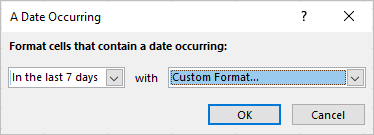
The second major way is using Conditional Formatting to check if the current date is before or after another date. Conditional Formatting is a very visual method of highlighting data that meets a certain condition in Excel. The A Date Occurring rule in Conditional Formatting provides a few earlier date options:
 7")
Using these preset options can highlight yesterday’s date or dates having occurred in the last 7 days, last week, or last month.
We will aim to highlight those dates in Excel that precede today’s date by a Conditional Formatting rule. Go through the steps below to see the rule we’re applying through Conditional Formatting to check if a date is before the current date:
- Select the cells with the dates that you want to check against today’s date.
- Select the Conditional Formatting icon from the Styles group in the Home
 8")
- From the menu, go to Highlight Cells Rules > Less Than.
 9")
- In the opened dialog box, type the following formula:
=TODAY()
- Use the next bar to set the format for the highlighted cells.
 10")
- The background of this rule is what we have seen in the earlier sections; checking the date to be less than the date today. From the selected cells, Conditional Formatting will highlight all the cells meeting this condition in Light Red Fill with Dark Red Text.
- Click on the OK button in the dialog box.
The dates falling before the 31st of October will be highlighted:
 11")
Let’s tweak the data a bit so that along with these highlighted 3 dates, we’ll have the date 28th October which will be the date furthest behind the 31st in the dataset. Leaving the previous Conditional Formatting rule as it is, 28th will then also be highlighted in light red. If we add another rule similar to the previous one, the only change is in the TODAY function as follows:
=TODAY()-2
This will highlight the dates less than 2 days from today and we’ve chosen red fill so it further stands out:
 12")
All days that are two or more days before today will be highlighted in red fill. However, make sure to keep the second rule in top preference otherwise the dates will only fall under the first rule. The preference can be changed in the Conditional Formatting Rules Manager.
 13")
This was how to use the TODAY function to highlight dates more than x days before the current date. E.g. highlighting the dates more than 2 weeks before the current date can be done with the Less Than rule with the following input formula:
=TODAY()-14
With the Between Highlight Cells rule, Conditional Formatting can highlight the dates occurring, let’s say, between 2 weeks to a week before today like so:
 14")
Conditional Formatting provides a very easily deducible visual, right? The longer dues in a darker shade. You can leave that all to Excel and set this up in a matter of seconds with Conditional Formatting‘s Color Scales option. To apply it, go to the Home tab > Conditional Formatting icon > Color Scales and choose a Color Scale. We’ve chosen a 2-Color Scale.
 15")
The Color Scale will be applied immediately highlighting the earliest date in red and shading the dates as per the Color Scale tones to the latest date in white.
 16")
While this is cool, it’s missing the TODAY component. We have a little trick to make this Color Scale relevant to the date today so head to the Rule Manager and edit the rule involving this Color Scale.
On the Maximum side that is represented by the white color, change the Type to Number. In the Value field, enter the TODAY function as:
=TODAY()
The purpose of these changes is to limit the Color Scale to just the current date instead of the latest date in the selected cells. Apply the changes with the OK command.
 17")
See the change in the Conditional Formatting? Now only the dates before the current date are prominent while the current date and beyond are white.
 18")
And here’s where we check out. That was our tutorial with some easy tricks on checking if a date is before today’s date in Excel where the TODAY function can play a very convenient role. While you’re getting your way around with dates, we’ll work on more Excel matter for your checking.
Содержание
- Excel IF Function With Dates
- Excel IF function combining with DATEVALUE function
- Excel IF function combining with DATE function
- Excel IF function combining with TODAY function
- Excel IF statement between two numbers or dates
- Excel formula: if between two numbers
- If between two numbers then
- If boundary values are in different columns
- Excel formula: if between two dates
- If date is within next N days
- If date is within last N days
- Practice workbook
- You may also be interested in
Excel IF Function With Dates
If you have a list of dates and then want to compare to these dates with a specified date to check if those dates is greater than or less than that specified date. You can use the IF function in combination with logical operators and DATEVALUE function in Microsoft excel.
Excel IF function combining with DATEVALUE function
Since that Excel cannot recognize the date formats and just interprets them as a text string. So you need to use DATAVALUE function and let Excel think that it is a Date value. For example: DATEVALUE(“11/3/2018”). Now we can write down the following IF formula with Dates.
The above excel IF formula will check the date value in Cell B1 if it is less than another specified date(11/3/2018), if the test is TRUE, then return “good”, otherwise return “bad”
Excel IF function combining with DATE function
You can also use DATE function in an Excel IF statement to compare dates, like the below IF formula:
The above IF formula will check if the value in cell B1 is less than or equal to 11/3/2018 and show the returned value in cell C1, Otherwise show nothing.
Excel IF function combining with TODAY function
If you want to compare the current date with the specified date in the past, you can use IF function in combination with TODAY function in Excel. Like the following IF formula:
We also can use the complex logical test using Today function, like this: B1-TODAY>10, it will check the date value in one cell if it is more than 10 days from now. Let’s combine this logical test in the IF formula as follow:
Источник
Excel IF statement between two numbers or dates
 by Alexander Frolov, updated on March 7, 2023
The tutorial shows how to use an Excel IF formula to see if a given number or date falls between two values.
To check if a given value is between two numeric values, you can use the AND function with two logical tests. To return your own values when both expressions evaluate to TRUE, nest AND inside the IF function. Detailed examples follow below.
Excel formula: if between two numbers
To test if a given number is between two numbers that you specify, use the AND function with two logical tests:
- Use the greater then (>) operator to check if the value is higher than a smaller number.
- Use the less than ( smaller_number, value =) and less than or equal to ( = smaller_number, value =AND(A2>10, A2
To check if A2 is between 10 and 20, including the threshold values, the formula in C2 takes this form:
In both cases, the result is the Boolean value TRUE if the tested number is between 10 and 20, FALSE if it is not:

If between two numbers then
In case you want to return a custom value if a number is between two values, then place the AND formula in the logical test of the IF function.
For example, to return «Yes» if the number in A2 is between 10 and 20, «No» otherwise, use one of these IF statements:
If between 10 and 20:
If between 10 and 20, including the boundaries:

Tip. Instead of hardcoding the threshold values in the formula, you can input them in individual cells, and refer to those cells like shown in the below example.
Suppose you have a set of values in column A and wish to know which of the values fall between the numbers in columns B and C in the same row. Assuming a smaller number is always in column B and a larger number is in column C, the task can be accomplished with this formula:
Including the boundaries:

And here is a variation of the If between statement that returns a value itself if TRUE, some text or an empty string if FALSE:
Including the boundaries:

If boundary values are in different columns
When smaller and larger numbers you are comparing against may appear in different columns (i.e. number 1 is not always smaller than number 2), use a slightly more complex version of the formula.
=AND(A2>=MIN(B2, C2), A2
To return your own values instead of TRUE and FALSE, use the following Excel IF statement between two numbers:
=IF(AND(A2>MIN(B2, C2), A2
=IF(AND(A2>=MIN(B2, C2), A2

Excel formula: if between two dates
The If between dates formula in Excel is essentially the same as If between numbers.
To check whether a given date is within a certain range, the generic formula is:

In case, the start and end dates are in predefined cells, the formula becomes much simpler:
Where $E$2 is the start date and $E$3 is the end date. Please notice the use of absolute references to lock the cell addresses, so the formula won’t break when copied to the below cells.

Tip. If each tested date should fall in its own range, and the boundary dates may be interchanged, then use the MIN and MAX functions to determine a smaller and larger date as explained in If boundary values are in different columns.
If date is within next N days
To test if a date is within the next n days of today’s date, use the TODAY function to determine the start and end dates. Inside the AND statement, the first logical test checks if the target date is greater than today’s date, while the second logical test checks if it is less than or equal to the current date plus n days:

If date is within last N days
To test if a given date is within the last n days of today’s date, you again use IF together with the AND and TODAY functions. The first logical test of AND checks if a tested date is greater than or equal to today’s date minus n days, and the second logical test checks if the date is less than today:

Hopefully, our examples have helped you understand how to use the If between formula in Excel efficiently. I thank you for reading and hope to see you on our blog next week!
Practice workbook
You may also be interested in
Table of contents
Hello!
Hope you can help me out — how to calculate how many B values in a repeating range A values with a range of 1 row.
For example: A B C B D A C B B D A A C B B D . here there are 3 ranges of A values and I need your help how to know how many B values in each interval.
Thank you so much!
Reply
Hi!
I don’t really understand in which ranges do you want to count characters. But I hope this guide will be helpful to you: How to count characters in Excel cell and range. If that’s not enough, explain the problem in more detail.
Hello, I wish to create an IF function that will provide me with variable results based on dates occurring before a date input directly into the formula. So, if C8, D8 and E8 are all less than 1/1/24, it give me one result, but if only 1 or 2 are before, I get different results based on how many dates are before the input date in the formula.
I am currently trying to get the following formula to work:
Hello!
To input the correct date in a formula, use DATE function. Read more in this manual: Excel DATE function with formula examples to calculate dates.
How do I place a formula to give 150 as result if gross salary is between kshs 0-6000, and formula to give 300 as result if gross salary is between ksh 6001- 8000, and the formula to give 400 as result if gross salary is between kshs 8001- 12000.
Hi!
You can find the answer to your question in this article: Nested IF in Excel – formula with multiple conditions
I need a formula to give me a fixed percentage based on two figures. Looking at the retirement fund lump sum withdrawal benefits tax income table (how much will the member be taxed on) I want to build a formula that once I put the person’s fund value in one cell it will show me the percentage taxable in another cell.
Table is as follow:
Between 1 — 27 500 = 0%
Between 27 501 — 726 000 = 18%
Between 726 001 — 1 089 000 = 27%
Between 1 089 001 and above = 36%
Hi!
Please check out the following article on our blog, it’ll be sure to help you with your task: Excel nested IF statement — multiple conditions in a single formula.
Firstly, thanks for the great content. It’s helped me a lot (but I’m stuck!)
I’m trying to compare 2 numbered lists.
In List A, I have a list of numbers ranging from 6-11 digits in length, where each cell (A2, An) is a unique number.
In List B, I have a different format, where column E & F are called Low Range & High Range respectively. It’s purpose is to create a range where the number is sequential and doesn’t break, if it breaks, it moves to the next range.
For Example:
The following numbers are depicted differently in both Lists below (200000, 200001, 200002, 200004, 200006, 200007, 200008, 200010)
List A:
Cell A2 = 200000
Cell A3 = 200001
Cell A4 = 200002
Cell A5 = 200004
Cell A6 = 200006
Cell A7 = 200007
Cell A8 = 200008
Cell A9 = 200010
List B:
Cell E2 (Low Range) = 200000 — Cell F2 (High Range) = 200002 (i.e. includes 200001)
Cell E3 (Low Range) = 200004 — Cell F3 (High Range) = 200004
Cell E4 (Low Range) = 200006 — Cell F4 (High Range) = 200008 (i.e. includes 200007)
Cell E5 (Low Range) = 200009 — Cell F5 (High Range) = 200009
Problem I’m trying to solve:
I’m trying to compare each cell (A2, An) in List A to each Low Range & High Range (Column E & F) combination. I have it working when I specify an individual cell in List A (A2) and compare it to E2 & F2 in List B using the following formula:
Hello!
If I understand your task correctly, the following formula should work for you:
You Sir are a genius! Many thanks Alexander!
Trying to get a formulae to work which will populate a cell.
If A2 is between 1-6 then in H2 will show Low, if A2 is between 7-12 then in H2 will show Medium, if A2 is between 13-16 then in H2 will show High,
Cell A2 is a formulae arrived from other cells
tried the If statements but don’t appear to work
Condition
From- 1-Jan-23 (to) 10-Jan-23
within A,B,C & D, i have to mention «YES» if «A» contains dates fulfilling the above condition or «No» . likewise for B,C & D. Kindly help.
A 5-Jan-23 to 10-Feb-23
B 11-Jan-23 to 10-Feb-23
C 1-Jan-23 to 7-Jan-23
D 11-Jan-23 to 10-Feb-23
Hello!
If I understand correctly, each date interval is written as text in a cell. You can’t do any calculations with text. You can apply the recommendations described in the article above only if each date is written in a separate cell. To split the text into separate cells, I recommend using this instruction: Split string by delimiter or pattern, separate text and numbers. Then convert the text to date as described in the article at the link.
Hello, I’m trying to create a spreadsheet which returns overdue, active and imminent using the following formula. How can I express that when the date is 6 it returns OVERDUE. At the moment the imminent command is cancelling out the dates which should return ACTIVE.
sorry, that didn’t make sense.
I want it to display IMMINENT when TODAY is 6 from the date in H3.
oh boy, I’m sorry, the formula keeps changing when I post .
I want it to display IMMINENT when TODAY is greater than 4 but less than 6 compared with the date in H3.
Hi!
Based on your description, it is hard to completely understand your task. However, I’ll try to guess and offer you the following formula:
Hi!
I’m sorry, I’m afraid these pieces of info are not enough to give you a formula. Describe in detail the criteria for each of the three options and I will try to help
Thank You Alexander,
What I’m trying to create is a list of duties which need to be completed every 7 days.
In the H column, I want members of my team to type in the date that they last did the duty.
If the date inputted is more than 7 days from TODAY, I want the column with the formula in to to display «OVERDUE»
If the date is less than 7 but more than 2 days from TODAY, I what it to display «ACTIVE»
If the date is 2 days before TODAY, I want it to display IMMINENT
I have inherited the formula below but it never displays «IMMINENT». I am trying to amend this formula so that 2 days before it says OVERDUE, It flags up that the duty is imminent.
Sorry, I hadn’t seen your 2.16 reply. I’m not sure my 2.30 message made sense. I’ve just trying the formula you suggested.
Hi!
Try this formula
I am trying to add comment Late or On time based on 2 dates: I have a column for due date and a column for actual date
If due date and actual date are the same or actual date is earlier — then its on time
If actual date is later than due date its late.
How would I build this please?
Hi!
Compare two dates using the IF function:
=IF(A1>=B1, «On time», «Late»)
I want to input in a cell:
if value in N3 is between 0 and 7, then «7 days», if between 0 and 14, then «14 days», if between 0 and 30, then «30 days», if between 0 and 60, then «60 days»
I would appreciate your help
Hi!
Pay attention to the first paragraph of the article above. It covers your case completely.
I’m trying to create myself a time sheet — if I work less than 8 hours, i get a 30 min lunch break and if i work more than 8 hours i get a 45 min lunch break. So I’ve played around with a lot of different ways to do this, what i think isnt working is trying to get it to return a value in minutes. This is where I’ve got (but this doesnt work):
=IFS(D2=timevalue»8:00″,timevalue»00:45″)
Hi!
Use the TIME function to get a specific time value.
i have an urgent column with yes or no, and a date column. I want to create a due date by adding either 2 days if yes and 7 days if no.
Hi!
For multiple conditions, you can use the IFS function
I want to have a formula of startdate-31/12/22 but if startdate if lower than 01/01/22 then it will be just 12
Hello, i have struggle to find a formula for this » if up to 70% then 80%,if between 50%-70% then 50% and if between 40%-50% then 40%. I need this all in one row.
Thank you
Hi!
The answer to your question can be found in this article: Nested IF in Excel – formula with multiple conditions.
I am struggling to have multiple formula to create a target date for task completion.
Column A has revision numbers of the document ranging from 0 to 4
Column B has start date
Column C should be target date (if Column A contains 0, the Column C should be +14 days, — formula is =IF(C4=1,WORKDAY.INTL(NB,7,16)). I would like to repeat the same formula with different C column values for at least 4 times.
Hi!
Your formula does not match your question. I’m sorry, I’m afraid these pieces of info are not enough to give you a formula. Describe in detail what problem you have, and I will try to help you.
I need to calculate commissions based on % of MSRP by product line.
The % off of MSRP can vary between these cutoff amounts. Ie, the % MSRP could be 94% or 73%, the amounts don’t always fall along these specific cutoff values but at these cutoff values, the commission rate changes:
Column on worksheet % of MSRP % of MSRP % of MSRP
Product Line = 100% >= 92.50% >= 75%
column S 9% 6% 3%
column T 9% 6% 3%
column U 1% 1% 1%
column V 4% 2% 1%
MSRP is in column AD
I need assistance with the formula to calculate the commission if a sale falls between these cutoffs.
Hi!
If I understand the problem correctly, you can find the necessary instructions in the article above, as well as in this guide: Excel Nested IF statement.
hi if you can pls help
A B C D E F G
Week # Week # Vendor Amount Date
Wed 12/8/2021 1 1 11/30/2021
Wed 12/22/2021 2 1 11/30/2021
Wed 1/5/2022 3 2 12/13/2021
Wed 1/19/2022 4 2 12/16/2021
Wed 2/2/2022 5 2 12/20/2021
Wed 2/16/2022 6 3 12/23/2021
Wed 3/2/2022 7 3 12/25/2021
column «A» has a list of dates Column «B» has a list of the week number now when I enter a date in Column «G» column «D» should find the correct «week #» from column «B»
Hi!
You can use the VLOOKUP formula to find the week number from a list of dates.
I also recommend paying attention to the WEEKNUM function to get the week number.
thank you for the quick reply
the week number i have in column «B» is not the standard week number
the date i have in column «G» is not in Column «A» since the date in column «G» is a date between 2 rows in column «A»
any other sugetions?
abe
Hi!
I am not sure I fully understand what you mean.
I am trying to display a text value if a number between 198.4 and 350.5 is displayed, but the formula is not working for me, I am entering this formula:
Hi!
Please read the above article carefully.
Instead of AND(C5>MIN199,C5 199,C5 Reply
Hello,
I swear I’ve done this before but can’t for the life of me recall. I have two tables:
Table 1: Column C = a number I enter, Column D = a corresponding text based on table 2
Table 2: Column A = a lower limit, Column B = an upper limit, Column C = text
What I’m looking to do is IF Table 1, C = 10, so it is >= Table 2 Column A and Reply
In essence, you build a formula as explained in the «If between two numbers then» example, but instead of the hardcoded values, supply the corresponding references.
Assuming your table 2 is on Sheet2 beginning in row 2, use the following formula for D2 in table 1:
I’m currently building a number sequence, using 5 columns and 50 rows. The numbers can’t >9 if so they should +1 to the next row.
for example you enter 51410 in the respective 5 columns and underneath it then starts counting up from 51410 to 51411 etc.
I have been using the IF(AND function however eventually this sequence counts up from 9 going over the maximum value of 9.
A2 = 8 A3 =9
B2 = IF(AND(F63>=9,E63>=9),»0″,E63+1)
B3 = IF(F63=9,»0″,SUM(F63,1))
is there any way around this.
Hi!
Sorry, I do not fully understand the task. I don’t see a relation between your question and the example. Write an example of the data you want to get. Try this instruction to create a sequence of numbers: SEQUENCE function in Excel — auto generate number series.
I would like to calculate how many instances of a word based on the date range formula — example below using November 2022 as range:
Column C contains dates
Column F contains word: high, medium or low
Date range I am happy with & returns a value: =COUNTIFS($C:$C,»>=01/11/2022″,$C:$C,» Reply
Hello!
Add one more condition to the COUNTIFS formula.
How can I do a nested If statement with one of the the look up variables is a #. I have tried using wild cards, but end up with the same results.
=IF((Z2-Y2)0,»Late», IF(OR(COUNTIF(Z2, «*»&»#»&»*»)), «not received «, «»)))
The z2 and Y2 are date fields. The result is the same for the # it says #value!
Hello!
The answer to your question can be found in this article: COUNTIF formulas with wildcard characters (partial match). I hope my advice will help you solve your task.
here is my dilemma, if this can be done in excel or not.
I created a poker tracker sheet in excel to track my winnings on freerolls I play in, on various poker sites.
Now,
in Column D is my buy in, column E is won bounty and column H is price I won, and in column J is client name.
Now, how can I calculate in column K for each separate site and track my winnings from each separate site in column K??
Is it possible??
I.e. IF client name is GG then total winnings are.
IF client name is PS then total winnings are.
I wish I could post a screenshot to explain better what I mean.
Hello!
To calculate a sum based on one or more criteria, use the SUMIFS function. Look for the example formulas here: Excel SUMIFS and SUMIF with multiple criteria – formula examples. This should solve your task.
Copyright © 2003 – 2023 Office Data Apps sp. z o.o. All rights reserved.
Microsoft and the Office logos are trademarks or registered trademarks of Microsoft Corporation. Google Chrome is a trademark of Google LLC.
Источник
The IF function is one of the most useful Excel functions. It is used to test a condition and return one value if the condition is TRUE and another if it is FALSE.
One of the most common applications of the IF function involves the comparison of values.
These values can be numbers, text, or even dates. However, using the IF statement with date values is not as intuitive as it may seem.
In this tutorial, I will demonstrate some ways in which you can use the IF function with date values.
Syntax and Usage of the IF Function in Excel
The syntax for the IF function is as follows:
IF(logical_test, [value_if_true], [value_if_false])
Here,
- logical_test is the condition or criteria that you want the IF function to test. The result of this parameter is either TRUE or FALSE
- value_if_true is the value that you want the IF function to return if the logical_test evaluates to TRUE
- value_if_false is the value that you want the IF function to return if the logical_test evaluates to FALSE
For example, say you want to write a statement that will return the value “yes” if the value in cell reference A2 is equal to 10, and “no” if it’s anything but 10.
You can then use the following IF function for this scenario:
=IF(A2=10,"yes","no")

Comparing Dates in Excel (Using Operators)
Unlike numbers and strings, comparison operators, when used with dates, have a slightly different meaning.
Here are some of the comparison operators that you can use when comparing dates, along with what they mean:
| Operator | What it Means When Using with Dates |
|---|---|
| < | Before the given date |
| = | Same as the date with which we are comparing |
| > | After the given date |
| <= | Same as or before the given date |
| >= | Same as or after the given date |
It may look like IF formulas for dates are the same as IF functions for numeric or text values, since they use the same comparison operators.
However, it’s not as simple as that.
Unfortunately, unlike other Excel functions, the IF function cannot recognize dates.
It interprets them as regular text values.
So you cannot use a logical test such as “>05/07/2021” in your IF function, as it will simply see the value “05/07/2021” as text.
Here are a few ways in which you can incorporate date values into your IF function’s logical_test parameter.
Using the IF Function with DATEVALUE Function
If you want to use a date in your IF function’s logical test, you can wrap the date in the DATEVALUE function.
This function converts a date in text format to a serial number that Excel can recognize as a date.
If you put a date within quotes, it is essentially a text or string value.
When you pass this as a parameter to the DATEVALUE function, it takes a look at the text inside the double quotes, identifies it as a date and then converts it to an actual Excel date value.
Let us say you have a date in cell A2, and you want cell B2 to display the value “done” if the date comes before or on the same date as “05/07/2021” and display “not done” otherwise.
You can use the IF function along with DATEVALUE in cell B2 as follows:
=IF(A2<DATEVALUE("05/07/2021"),"done","not done")
Here’s a screenshot to illustrate the effect of the above formula:

Using the IF Function with the TODAY Function
If you want to compare a date with the current date, you can use the IF function with the TODAY function in the logical test.
Let’s say you have a date in cell A2 and you want cell B2 to display the value “done” if it is a date before today’s date.
If not, you want let’s say you want to display the value “not done”. You can use the IF function along with the TODAY function in cell B2 as follows:
=IF(A2<TODAY(),"done","not done")
Here’s a screenshot to illustrate the effect of the above formula (assuming the current date is 05/08/2021):

Using the IF Function with Future or Past Dates
An interesting thing about dates in Excel is that you can perform addition and subtraction operations with them too.
This is because dates are basically stored in Excel as serial numbers, starting from the date Jan 1, 1900.
Each day after that is represented by one whole number.
So, the serial number 2 corresponds to Jan 2, 1900, and so on.
This means that adding n number of days to a date is equivalent to adding the value n to the serial number that the date represents.
If TODAY() is 05/07/2021, then TODAY()+5 is five days after today, or 05/12/2021. Similarly, TODAY()-3 is three days before today or 05/04/2021.
Let’s say you have a date in cell A2 and you want cell B2 to mark it as “within range” if it is within 15 days from the current date.
If not, you want to show “out of range”. You can use the IF function along with the TODAY function in cell B2 as follows:
=IF(A2<TODAY()+15,"within range","out of range")
Here’s a screenshot to illustrate the effect of the above formula (assuming the current date is 05/08/2021):

Points to Remember
Having discussed different ways to use dates with the IF function, here are some important points to remember:
- Instead of hardcoding the dates into the IF function’s logical test parameter, you can store the date in a separate cell and refer to it with a cell reference. For example, instead of typing =IF(A2<”05/07/2021”,”done”,”not done”), you can store the date 05/07/2021 in a cell, say B2 and type the formula: =IF(A2<B2,”done”,”not done”).

- Alternatively, you can use the DATEVALUE function as explained in the first part of this tutorial.

- Another neat technique that you can use is to simply add a zero to the date (which has been enclosed in double quotes). So you can type: =IF(A2<”05/07/2021”+0,”done”,”not done”). This will make Excel take the date inside double quotes as a serial number, and use it in the logical test without having its value changed.

In this tutorial, I showed you some great techniques to use the IF function with dates. I hope the tips covered here were useful for you.
Other articles you may also like:
- Multiple If Statements in Excel (Nested Ifs, AND/OR) with Examples
- How to use Excel If Statement with Multiple Conditions Range [AND/OR]
- How to Convert Month Number to Month Name in Excel
- Why are Dates Shown as Hashtags in Excel? Easy Fix!
- How to Convert Serial Numbers to Date in Excel
- How to Get the First Day Of The Month In Excel?
Highlight Dates Before Today or Within a Date Range in Excel Using Conditional Formatting
by Avantix Learning Team | Updated October 17, 2022
Applies to: Microsoft® Excel® 2010, 2013, 2016, 2019, 2021 and 365 (Windows)
You can use conditional formatting in Excel to highlight cells containing dates before today or within a date range before the current date. In a worksheet, you can use conditional formatting to highlight selected cells by filling them with a color based on rules or conditions. This type of formatting is helpful if you want to highlight past due dates such as invoices that are 30, 60 or 90 days overdue.
When you apply conditional formatting, you can apply more than one rule to a range of cells.
In this article, we’ll review 3 ways to highlight dates before today using conditional formatting:
- Use built-in conditional formatting
- Create a conditional formatting rule based on cell contents
- Create a conditional formatting rule using a formula
Recommended article: How to Delete Blank Rows in Excel (5 Easy Ways with Shortcuts)
Do you want to learn more about Excel? Check out our virtual classroom or in-person Excel courses >
Dates must be entered or returned as valid dates in Excel in order to apply conditional formatting. Dates are affected by your regional settings and date / time settings in your Control Panel on your device.
For example, if your regional settings are set to U.S., dates are typically entered as mm/dd/yy (month / day / year) unless the date / time settings have been changed. For example, November 14, 2021 may be entered at 11/14/21 if your device’s regional settings are set to U.S (you can also enter dates with dashes such as mm-dd-yy). To test your device to see how dates are recognized, press Ctrl + ; (semi-colon) in a cell in an Excel worksheet to enter the current date in the cell. Dates can then be formatted to appear in a different ways.
The current date can also be entered in a cell using the TODAY function such as =TODAY() or the NOW function such as =NOW(). The NOW function enters the current date and time whereas the TODAY function only enters the current date. They are dynamic functions so will always display the current date.
Highlight dates before today using built-in conditional formatting
To highlight dates before today using a built-in conditional formatting rule:
- Select the cells containing dates to which you want to apply conditional formatting.
- Click the Home tab in the Ribbon.
- Click Conditional Formatting in the Styles group. A menu appears to the right.
- Select Highlight Cell Rules. A menu appears.
- From the drop-down menu, choose Dates Occurring. A dialog box appears.
- From the first drop-down menu, select an option such as Yesterday, In the last 7 days, Last Week, or Last Month.
- In the second drop-down menu beside With, select Custom Format. A dialog box appears.
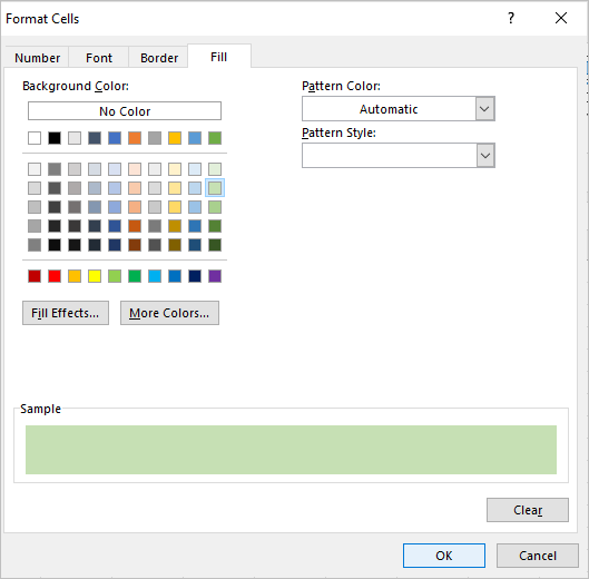
- Click the Fill tab and then click the desired fill color. You can also click the Font tab and select a font color or another format such as bold.
- Click OK twice.
The Date Occurring dialog box appears as follows with In the last 7 days selected (this option would include the current date):
In the Format Cells dialog box, you can select a fill as the conditional format:
Highlight dates before today by creating a conditional formatting rule based on cell contents
You can also apply your own formatting rules based on cell contents. This method gives you more control over how cells are formatted and allows you to do things you wouldn’t be able to do with the built-in formats.
To highlight dates before today by creating a conditional formatting rule based on cell contents:
- Select the cells containing dates to which you want to apply conditional formatting.
- Click the Home tab in the Ribbon.
- Click Conditional Formatting in the Styles group. A drop-down menu appears.
- Select New Rule. A dialog box appears.
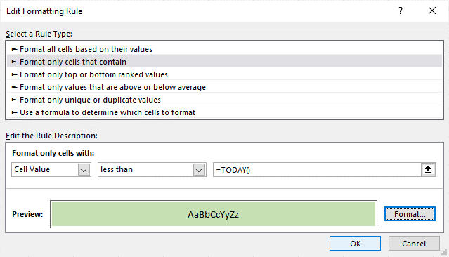
- Select Format only cells that contain.
- Below Format only cells with, ensure Cell Value is selected.
- From the second drop-down menu, select less than.
- In the text box, enter =TODAY().
- Click Format. A dialog box appears.
- Click the Fill tab and then click the desired fill color. You can also click the Font tab and select a font color or another format such as bold.
- Click OK twice.
In the Edit Formatting Rule dialog box below, we entered a rule to highlight the selected cells if the cell value is less than =TODAY():
To highlight cells containing a range of dates between today and a date in the past (not including today):
- Select the cells containing dates to which you want to apply conditional formatting.
- Click the Home tab in the Ribbon.
- Click Conditional Formatting in the Styles group. A drop-down menu appears.
- Select New Rule from the drop-down menu.
- Select Format only cells that contain.
- Below Format only cells with, ensure Cell Value is selected.
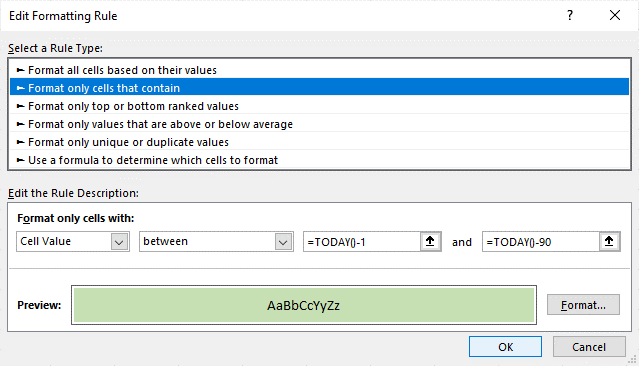
- From the second drop-down menu, select Between.
- In the first text box, enter =TODAY()-1.
- In the second text box, enter another date or formula. For example, if you are looking for dates in the last 90 days before the current date, enter =TODAY()-90. For 30 days overdue, enter =TODAY()-30.
- Click Format. A dialog box appears.
- Click the Fill tab and then click the desired fill color. You can also click the Font tab and select a font color or another format such as bold.
- Click OK twice.
In the Edit Formatting Rule dialog box below, we entered a rule to highlight the selected cells if the cell value is between =TODAY()-1 and =TODAY()-90 (within 90 days before the current date):
Highlight dates before today by creating a conditional formatting rule using a formula
You can use a variety of formulas in conditional formatting to change cell formats based on a formula.
When you are writing formulas in conditional formatting rules, context is very important. Write the formula as if you are in the active cell (often the first cell) and Excel, by default, uses relative referencing to copy the formula to the other cells.
To highlight dates before today by creating a conditional formatting rule using a formula:
- Select the cells in a column containing dates to which you want to apply conditional formatting.
- Click the Home tab in the Ribbon.
- Click Conditional Formatting in the Styles group. A drop-down menu appears.
- Select New Rule from the drop-down menu.
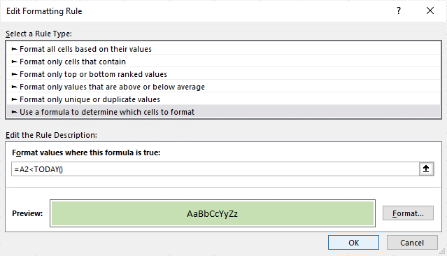
- Click Use a formula to determine which cells to format.
- Enter the formula (starting with =) in the formula box (the formula references the active cell which is usually the first cell and the conditional formatting tool will adjust it for the other cells if relative referencing is used). For example, enter =A2<TODAY() if A2 is the first in the range of selected cells containing a date.
- Click Format. A dialog box appears.
- Click the Fill tab and then click the desired fill color. You can also click the Font tab and select a font color or another format such as bold.
- Click OK twice.
In the Edit Formatting Rule dialog box below, we entered a formula rule of =A2<TODAY() to highlight the selected cells if the cell value is before today:
You can also use absolute and mixed referencing in conditional formatting rules.
If you want to highlight selected cells in a row with conditional formatting, select the range of cells across multiple columns and use a mixed reference with a dollar sign ($) in front of the column reference in the formula. For example, enter =$A2<TODAY() to highlight selected cells in a row before today.
Subscribe to get more articles like this one
Did you find this article helpful? If you would like to receive new articles, JOIN our email list.
More resources
How to Combine Cells in Excel Using Concatenate (3 Ways)
How to Insert Multiple Rows in Excel (4 Fast Ways with Shortcuts)
3 Excel Strikethrough Shortcuts to Cross Out Text or Values in Cells
How to Replace Blank Cells in Excel with a Value from the Cell Above
10 Excel Flash Fill Examples (Extract, Combine, Clean and Format Data with Flash Fill)
Related courses
Microsoft Excel: Intermediate / Advanced
Microsoft Excel: Data Analysis with Functions, Dashboards and What-If Analysis Tools
Microsoft Excel: Introduction to Visual Basic for Applications (VBA)
VIEW MORE COURSES >
Our instructor-led courses are delivered in virtual classroom format or at our downtown Toronto location at 18 King Street East, Suite 1400, Toronto, Ontario, Canada (some in-person classroom courses may also be delivered at an alternate downtown Toronto location). Contact us at info@avantixlearning.ca if you’d like to arrange custom instructor-led virtual classroom or onsite training on a date that’s convenient for you.
Copyright 2023 Avantix® Learning
Microsoft, the Microsoft logo, Microsoft Office and related Microsoft applications and logos are registered trademarks of Microsoft Corporation in Canada, US and other countries. All other trademarks are the property of the registered owners.
Avantix Learning |18 King Street East, Suite 1400, Toronto, Ontario, Canada M5C 1C4 | Contact us at info@avantixlearning.ca
Skip to content
На первый взгляд может показаться, что функцию ЕСЛИ для работы с датами можно применять так же, как для числовых и текстовых значений, которые мы только что обсудили. К сожалению, это не так.
Примеры работы функции ЕСЛИ с датами.
Дата в качестве условия, с которым работает функция ЕСЛИ, может быть записана в какую-то ячейку Excel, либо же прямо вставлена в формулу. Вот тут-то и возникают некоторые особенности и сложности работы функции ЕСЛИ с датами.
Пример 1. Формула условия для дат с
функцией ДАТАЗНАЧ (DATEVALUE)
Иногда случается, что записать дату непосредственно в функцию ЕСЛИ, не ссылаясь ни на какую ячейку. В этом случае возникают некоторые сложности.
В отличие от многих
других функций Excel, ЕСЛИ не может распознавать даты и интерпретирует их как текст,
как простые текстовые строки.
Поэтому вы не можете выразить свое логическое условие просто как >«15.07.2019» или же >15.07.2019. Увы, ни один из приведенных вариантов не верен.
Чтобы функция ЕСЛИ распознала дату в вашем логическом условии именно как дату, вы должны обернуть ее в функцию ДАТАЗНАЧ (в английском варианте – DATEVALUE).
Например, ДАТАЗНАЧ(«15.07.2019»).
Полная формула ЕСЛИ может
иметь следующую форму:
=ЕСЛИ(B2<ДАТАЗНАЧ(«10.09.2019″),»Поступил»,»Ожидается»)

Как показано на скриншоте,
эта формула ЕСЛИ оценивает даты в столбце В и возвращает «Послупил», если дата
поступления до 10 сентября. В противном случае формула возвращает «Ожидается».
Пример 2. Формула условия для дат с
функцией СЕГОДНЯ()
В случае, когда даты записаны в ячейки таблицы Excel, применять ДАТАЗНАЧ нет необходимости.
Если вы основываете свое условие на текущей дате, то можете взять функцию СЕГОДНЯ (в английском варианте — TODAY) в качестве аргумента функции ЕСЛИ.
К примеру, сегодня — 9 сентября 2019 года.
В столбце C отметим товар, который уже поступил. В ячейке C2 запишем:
=ЕСЛИ(B2<СЕГОДНЯ(),»Поступил»,»»)
В столбце D отметим товар, который еще не поступил. В ячейке D2 запишем:
=ЕСЛИ(B2<СЕГОДНЯ(),»»,»Ожидается»)

Пример 3. Расширенные
формулы ЕСЛИ для будущих и прошлых дат
Предположим, вы хотите
отметить только те даты, которые отстоят от текущей более чем на 30 дней.
Выделим даты, отстоящие более чем на месяц от текущей, в прошлом. Укажем для них «Более месяца назад». Запишем это условие:
=ЕСЛИ(СЕГОДНЯ()-B2>30,»Более
месяца назад»,»»)
Если условие не выполнено, то в ячейку запишем пустую строку «».
А для будущих дат, также отстоящих более чем на месяц, укажем «Ожидается».
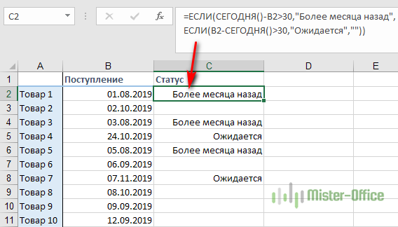
=ЕСЛИ(B2-СЕГОДНЯ()>30,»Ожидается»,»»)

Если все результаты попробовать объединить в одном столбце, то придется составить выражение с несколькими вложенными функциями ЕСЛИ:
=ЕСЛИ(СЕГОДНЯ()-B2>30,»Более месяца назад», ЕСЛИ(B2-СЕГОДНЯ()>30,»Ожидается»,»»))
Примеры работы функции ЕСЛИ: