
Excel for Microsoft 365 Excel for Microsoft 365 for Mac Excel for the web Excel 2021 Excel 2021 for Mac Excel 2019 Excel 2019 for Mac Excel 2016 Excel 2016 for Mac Excel 2013 Excel 2010 Excel 2007 Excel for Mac 2011 Excel Starter 2010 More…Less
You use the SUMIF function to sum the values in a range that meet criteria that you specify. For example, suppose that in a column that contains numbers, you want to sum only the values that are larger than 5. You can use the following formula: =SUMIF(B2:B25,»>5″)

This video is part of a training course called Add numbers in Excel.
Tips:
-
If you want, you can apply the criteria to one range and sum the corresponding values in a different range. For example, the formula =SUMIF(B2:B5, «John», C2:C5) sums only the values in the range C2:C5, where the corresponding cells in the range B2:B5 equal «John.»
-
To sum cells based on multiple criteria, see SUMIFS function.
Important: The SUMIF function returns incorrect results when you use it to match strings longer than 255 characters or to the string #VALUE!.
Syntax
SUMIF(range, criteria, [sum_range])
The SUMIF function syntax has the following arguments:
-
range Required. The range of cells that you want evaluated by criteria. Cells in each range must be numbers or names, arrays, or references that contain numbers. Blank and text values are ignored. The selected range may contain dates in standard Excel format (examples below).
-
criteria Required. The criteria in the form of a number, expression, a cell reference, text, or a function that defines which cells will be added. Wildcard characters can be included — a question mark (?) to match any single character, an asterisk (*) to match any sequence of characters. If you want to find an actual question mark or asterisk, type a tilde (~) preceding the character.
For example, criteria can be expressed as 32, «>32», B5, «3?», «apple*», «*~?», or TODAY().
Important: Any text criteria or any criteria that includes logical or mathematical symbols must be enclosed in double quotation marks («). If the criteria is numeric, double quotation marks are not required.
-
sum_range Optional. The actual cells to add, if you want to add cells other than those specified in the range argument. If the sum_range argument is omitted, Excel adds the cells that are specified in the range argument (the same cells to which the criteria is applied).
Sum_range
should be the same size and shape as range. If it isn’t, performance may suffer, and the formula will sum a range of cells that starts with the first cell in sum_range but has the same dimensions as range. For example:
range
sum_range
Actual summed cells
A1:A5
B1:B5
B1:B5
A1:A5
B1:K5
B1:B5
Examples
Example 1
Copy the example data in the following table, and paste it in cell A1 of a new Excel worksheet. For formulas to show results, select them, press F2, and then press Enter. If you need to, you can adjust the column widths to see all the data.
|
Property Value |
Commission |
Data |
|---|---|---|
|
$100,000 |
$7,000 |
$250,000 |
|
$200,000 |
$14,000 |
|
|
$300,000 |
$21,000 |
|
|
$400,000 |
$28,000 |
|
|
Formula |
Description |
Result |
|
=SUMIF(A2:A5,»>160000″,B2:B5) |
Sum of the commissions for property values over $160,000. |
$63,000 |
|
=SUMIF(A2:A5,»>160000″) |
Sum of the property values over $160,000. |
$900,000 |
|
=SUMIF(A2:A5,300000,B2:B5) |
Sum of the commissions for property values equal to $300,000. |
$21,000 |
|
=SUMIF(A2:A5,»>» & C2,B2:B5) |
Sum of the commissions for property values greater than the value in C2. |
$49,000 |
Example 2
Copy the example data in the following table, and paste it in cell A1 of a new Excel worksheet. For formulas to show results, select them, press F2, and then press Enter. If you need to, you can adjust the column widths to see all the data.
|
Category |
Food |
Sales |
|---|---|---|
|
Vegetables |
Tomatoes |
$2,300 |
|
Vegetables |
Celery |
$5,500 |
|
Fruits |
Oranges |
$800 |
|
Butter |
$400 |
|
|
Vegetables |
Carrots |
$4,200 |
|
Fruits |
Apples |
$1,200 |
|
Formula |
Description |
Result |
|
=SUMIF(A2:A7,»Fruits»,C2:C7) |
Sum of the sales of all foods in the «Fruits» category. |
$2,000 |
|
=SUMIF(A2:A7,»Vegetables»,C2:C7) |
Sum of the sales of all foods in the «Vegetables» category. |
$12,000 |
|
=SUMIF(B2:B7,»*es»,C2:C7) |
Sum of the sales of all foods that end in «es» (Tomatoes, Oranges, and Apples). |
$4,300 |
|
=SUMIF(A2:A7,»»,C2:C7) |
Sum of the sales of all foods that do not have a category specified. |
$400 |
Top of Page
Need more help?

See also
SUMIFS function
COUNTIF function
Sum values based on multiple conditions
How to avoid broken formulas
VLOOKUP function
Need more help?
На чтение 2 мин
Функция СУММЕСЛИ (SUMIF) в Excel используется для суммирования значений, отвечающих заданным вами критериям.
Содержание
- Что возвращает функция
- Синтаксис
- Аргументы функции
- Дополнительная информация
- Примеры использования функции СУММЕСЛИ в Excel
Что возвращает функция
Возвращает сумму чисел, указанных в качестве аргументов и отвечающих заданным в формуле критериям.
 Больше лайфхаков в нашем Telegram Подписаться
Синтаксис
=SUMIF(range, criteria [sum_range]) — английская версия
=СУММЕСЛИ(диапазон; условие; [диапазон_суммирования]) — русская версия
Аргументы функции
- range (диапазон) — диапазон ячеек, по которым оцениваются критерии. Аргументом могут быть числа, текст, массивы или ссылки, содержащие числа;
- criteria (условие) — критерии, которые проверяются по указанному диапазону ячеек и определяют, какие ячейки суммировать;
- sum_range (диапазон_суммирования) — (не обязательно) суммируемые ячейки. Если этот аргумент не указан, то функция использует аргумент range (диапазон) в качестве sum_range (диапазон_суммирования).
Дополнительная информация
- суммирование ячеек в функции СУММЕСЛИ производится на основе одного критерия, если вам необходимо указать несколько критериев — используйте функцию SUMIFS (СУММЕСЛИМН);
- пустые и текстовые ячейки в аргументе sum_range (диапазон_суммирования) игнорируются;
- критерием для функции могут служить числа, выражения, результаты вычисления из других ячеек, текст или формула;
- если в качестве критерия указан текст или математический/логический символ (=,+,-,/,*), то такие значения должны быть указаны в двойных кавычках;
- аргумент с критерием не должен быть длиннее чем 255 символов;
- в качестве критерия могут использоваться подстановочные знаки (*);
- если количество ячеек в диапазоне критерия и аргументе sum_range (диапазон_суммирования) различаются, то размер диапазона критерия будет в приоритете.
Примеры использования функции СУММЕСЛИ в Excel
Содержание
- Sum values based on multiple conditions
- Give it a try
- How to use a logical AND or OR in a SUM+IF statement in Excel
- Summary
- More Information
- Example
- References
- SUMPRODUCT with IF
- Related functions
- Summary
- Generic formula
- Explanation
- Basic SUMPRODUCT
- SUMPRODUCT + IF function
- SUMPRODUCT + Boolean logic
- Simplifying with a single array
- How to use SUMIF function in Excel with formula examples
- SUMIF in Excel — syntax and basic uses
- Basic SUMIF formula
- How to use SUMIF in Excel — formula examples
- SUMIF greater than or less than
- SUM IF equal to
- SUM IF not equal to
- SUM IF blank
- SUM IF not blank
- Excel SUMIF with text criteria
- SUMIF formulas with wildcard characters
- Example 1. Sum values based on partial match
- Example 2. Sum if cell contains * or ?
- Example 3. Sum if another cell contains text
- How to use Excel SUMIF with dates
- How to do SUMIF from another sheet
- How to correctly use cell references in SUMIF criteria
- Why is my SUMIF formula not working?
- 1. SUMIF supports only one condition
- 2. Range and sum_range should be of the same size
- 3. Range and sum_range should be ranges, not arrays
- 5. SUMIF criteria syntax
- 4. SUMIF from another workbook not working
- 6. SUMIF does not recognize text case
Sum values based on multiple conditions
Let’s say that you need to sum values with more than one condition, such as the sum of product sales in a specific region. This is a good case for using the SUMIFS function in a formula.
Have a look at this example in which we have two conditions: we want the sum of Meat sales (from column C) in the South region (from column A).
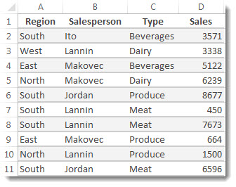
Here’s a formula you can use to acomplish this:
The result is the value 14,719.
Let’s look more closely at each part of the formula.
=SUMIFS is an arithmetic formula. It calculates numbers, which in this case are in column D. The first step is to specify the location of the numbers:
In other words, you want the formula to sum numbers in that column if they meet the conditions. That cell range is the first argument in this formula—the first piece of data that the function requires as input.
Next, you want to find data that meets two conditions, so you enter your first condition by specifying for the function the location of the data (A2:A11) and also what the condition is—which is “South”. Notice the commas between the separate arguments:
Quotation marks around “South” specify that this text data.
Finally, you enter the arguments for your second condition – the range of cells (C2:C11) that contains the word “meat,” plus the word itself (surrounded by quotes) so that Excel can match it. End the formula with a closing parenthesis ) and then press Enter. The result, again, is 14,719.
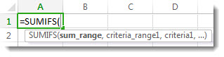
As you type the SUMIFS function in Excel, if you don’t remember the arguments, help is ready at hand. After you type =SUMIFS(, Formula AutoComplete appears beneath the formula, with the list of arguments in their proper order.
Looking at the image of Formula AutoComplete and the list of arguments, in our example sum_rangeis D2:D11, the column of numbers you want to sum; criteria_range1is A2.A11, the column of data where criteria1 “South” resides.
As you type, the rest of the arguments will appear in Formula AutoComplete (not shown here); criteria_range2 is C2:C11, the column of data where criteria2 “Meat” resides.
If you click SUMIFS in Formula AutoComplete, an article opens to give you more help.
Give it a try
If you want to experiment with the SUMIFS function, here’s some sample data and a formula that uses the function.
You can work with sample data and formulas right here, in this Excel for the web workbook. Change values and formulas, or add your own values and formulas and watch the results change, live.
Copy all the cells in the table below, and paste into cell A1 in a new worksheet in Excel. You may want to adjust column widths to see the formulas better
Источник
How to use a logical AND or OR in a SUM+IF statement in Excel
Summary
In Microsoft Excel, when you use the logical functions AND and/or OR inside a SUM+IF statement to test a range for more than one condition, it may not work as expected. A nested IF statement provides this functionality; however, this article discusses a second, easier method that uses the following formulas.
For AND Conditions
For OR Conditions
More Information
Use a SUM+IF statement to count the number of cells in a range that pass a given test or to sum those values in a range for which corresponding values in another (or the same) range meet the specified criteria. This behaves similarly to the DSUM function in Microsoft Excel.
Example
This example counts the number of values in the range A1:A10 that fall between 1 and 10, inclusively.
To accomplish this, you can use the following nested IF statement:
The following method also works and is much easier to read if you are conducting multiple tests:
The following method counts the number of dates that fall between two given dates:
- You must enter these formulas as array formulas by pressing CTRL+SHIFT+ENTER simultaneously. On the Macintosh, press COMMAND+RETURN instead.
- Arrays cannot refer to entire columns.
With this method, you are multiplying the results of one logical test by another logical test to return TRUEs and FALSEs to the SUM function. You can equate these to:
The method shown above counts the number of cells in the range A1:A10 for which both tests evaluate to TRUE. To sum values in corresponding cells (for example, B1:B10), modify the formula as shown below:
You can implement an OR in a SUM+IF statement similarly. To do this, modify the formula shown above by replacing the multiplication sign (*) with a plus sign (+). This gives the following generic formula:
References
For more information about how to calculate a value based on a condition, click Microsoft Excel Help on the Help menu, type about calculating a value based on a condition in the Office Assistant or the Answer Wizard, and then click Search to view the topic.
Источник
SUMPRODUCT with IF
Summary
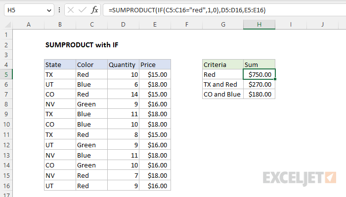
To create a conditional sum with the SUMPRODUCT function you can use the IF function or use Boolean logic. In the example shown, the formula in H5 is:
The result is $750, the total value of items with a color of «Red» in the data as shown. Note that SUMPRODUCT is not case-sensitive. Using the IF function inside SUMPRODUCT makes this into an array formula that must be entered with control + shift + enter in Legacy Excel. See below for an alternative Boolean syntax that does not need special handling.
Generic formula
Explanation
In this example, the goal is to calculate a conditional sum with the SUMPRODUCT function to match the criteria shown in G5:G7. One way to do this is to use the IF function directly inside of SUMPRODUCT. Another more common alternative is to use Boolean logic to apply criteria. Both approaches are explained below.
Basic SUMPRODUCT
The SUMPRODUCT function multiplies ranges or arrays together and returns the sum of products. The classic SUMPRODUCT problem multiplies two ranges together and sums the product directly without a helper column. For example, in the worksheet above, we have Quantity and Price, but no line item total. You can use SUMPRODUCT to get the total value of all records in the data like this:
In the worksheet shown, the result is $1,882, the sum of all quantities in D5:D16 multiplied by all prices in E5:E16. This formula works nicely. However, it’s not obvious how to calculate a conditional sum with SUMPRODUCT. For example, how can you calculate the value of all records where the color is «Red»? One option is to use the IF function directly, as explained in the next section.
SUMPRODUCT + IF function
One way to apply conditions with the SUMPRODUCT function is to use the IF function directly. This is the approach seen in the worksheet shown, where the formula in cell H5 is:
In this configuration, SUMPRODUCT has been given three arguments, array1, array2, and array3. Note that array2 holds Quantity and array3 holds Price. It is array1 that applies the conditional logic with the IF function like this:
Notice we are using 1 and 0 for the value_if_true and value_if_false arguments instead of the default TRUE and FALSE values. We do this because we want a numeric result, for reasons that become clear below. Because there are 12 values in the range C5:C16, IF returns an array with 12 results like this:
In this array, 1s indicate records where the color is «Red» and 0s indicate other colors. Dropping this array back into the SUMPRODUCT function, we have:
Now you can see how the logic works. The Boolean values that make up array1 act like a filter when the arrays are multiplied together. After multiplication, there is just a single array like this:
Note that the value of records where the color is not «Red» have been «zeroed out». The final result returned by SUMPRODUCT is $750. Additional conditions can be added with additional IF statements. To calculate a total for Color = «Red» and State = «TX», you can use the IF function twice like this:
The result is $270, as you can see in cell H6. The formula in cell H7 calculates a total for color = «Blue» and State = «CO» like this:
Although this formula works fine, one consequence of using the IF function inside of SUMPRODUCT is that it makes this into an array formula that must be entered with control + shift + enter in older versions of Excel that do not support dynamic array formulas. This is a bit unexpected, because one of SUMPRODUCT’s key strengths is the ability to handle array operations natively, but the IF function defeats this feature. The traditional solution to this problem is to switch to Boolean logic, as explained below.
SUMPRODUCT + Boolean logic
An alternative to using the IF function directly inside of SUMPRODUCT is to use Boolean logic. For example, to calculate the total value of records where the color is «Red», you can use a formula like this:
This example illustrates one of the key strengths of the SUMPRODUCT function – the ability to handle array operations natively. Inside SUMPRODUCT, the first array is a logical expression to filter on the color «red»:
SUMPRODUCT is not case-sensitive, so «red» will match «red», «Red», and «RED». Because there are 12 values in the range C5:C16, this expression returns an array with 12 results like this:
The double negative (—) then converts the TRUE and FALSE values to 1s and zeros:
Back in SUMPRODUCT, we now have:
Notice this is the same result we had with the IF function example above. As before, array1 acts like a filter when the arrays are multiplied together. After multiplication, there is just a single array like this:
All values associated with colors that are not «Red» have been «zeroed out», and the final result is $750. As with the IF function, the same pattern can be repeated to add more conditions. To calculate a total for Color = «Red» and State = «TX», you can use a formula like this:
To calculate a total for color = «Blue» and State = «CO», the formula is:
Simplifying with a single array
Excel pros will often simplify the syntax inside SUMPRODUCT by placing the conditional logic into a single argument like this
One advantage of this approach is that the math operation in array1 automatically coerces TRUE and FALSE into 1s and 0s, so we don’t need a double negative (—). Another advantage is that the math operation can be changed to apply a different type of logic. Instead of multiplication (*), which corresponds to AND logic in Boolean algebra, you can use addition (+), which corresponds to OR logic. For example, to sum the value of all records that are either «Red» or «Blue», you could use a formula like this:
As you can see, using Boolean logic with SUMPRODUCT is a flexible alternative to using the IF function, and it offers a major advantage: the formula will work fine in Legacy Excel, with no need to enter as an array formula with control + shift + enter.
Источник
How to use SUMIF function in Excel with formula examples
 by Svetlana Cheusheva, updated on November 11, 2022
This tutorial explains the Excel SUMIF function in plain English. The main focus is on real-life formula examples with all kinds of criteria including text, numbers, dates, wildcards, blanks and non-blanks.
Microsoft Excel has a handful of functions to summarize large data sets for reports and analyses. One of the most useful functions that can help you make sense of an incomprehensible set of diverse data is SUMIF. Instead of adding up all numbers in a range, it lets you sum only those values that meet your criteria.
So, whenever your task requires conditional sum in Excel, the SUMIF function is what you need. A good thing is that the function is available in all versions, from Excel 2000 through Excel 365. Another great thing is that once you’ve learned SUMIF, it will take you very little effort to master other «IF» functions such as SUMIFS, COUNTIF, COUNTIFS, AVERAGEIF, etc.
SUMIF in Excel — syntax and basic uses
The , also known as Excel conditional sum, is used to add up cell values based on a certain condition.
The function is available in Excel 365, Excel 2021, Excel 2019, Excel 2016, Excel 2013, Excel 2010, Excel 2007, and lower.
The syntax is as follows:
As you see, the SUMIF function has 3 arguments — first 2 are required and the last one is optional.
- Range (required) — the range of cells to be evaluated by criteria.
- Criteria (required) — the condition that must be met. It may be supplied in the form of a number, text, date, logical expression, a cell reference, or another Excel function. For example, you can enter the criteria such as «5», «cherries», «10/25/2014″, » Note. Please pay attention that any text criteria or criteria containing logical operators must be enclosed in double quotation marks, e.g. «apples», «>10». Cell references should be used without the quotation marks, otherwise they would be treated as text strings.
Basic SUMIF formula
To better understand the SUMIF syntax, consider the following example. Suppose you have a list of products in column A, regions in column B, and sales amounts in column C. Your goal is to get a total of sales for a specific region, say North. To have it done, let’s build an Excel SUMIF formula in its simplest form.
You start with defining the following arguments:
- Range — a list of regions (B2:B10).
- Criteria — «North» or a cell containing the region of interest (F1).
- Sum_range — the sales amounts to be added up (C2:C10).
Putting the arguments together, we get the following formula:
=SUMIF(B2:B10, «north», C2:C10)
=SUMIF(B2:B10, F1, C2:C10)
Both formulas only sum sales in the North region: 
Note. The sum_range parameter actually defines only the upper leftmost cell of the range to be summed. The remaining area is defined by the dimensions of the range argument. In practice, this means that sum_range argument does not necessarily have to be of the same size as range argument, i. e. it may have a different number of rows and columns. However, the top left cell must always be the right one. For example, in the above formula, you can supply C2, or C2:C4, or even C2:C100 as the sum_range argument, and the result will still be correct. However, the best practice is to provide equally sized range and sum_range.
Note. The SUMIF function is case-insensitive by nature. However, it is possible to force it to recognize the text case. For full details, please see Case-sensitive SUMIF in Excel.
How to use SUMIF in Excel — formula examples
Hopefully, the above example has helped you gain some basic understanding of how the function works. Below you will find a few more formulas that demonstrate how to use SUMIF in Excel with various criteria.
SUMIF greater than or less than
To sum numbers greater than or less than a particular value, configure the SUMIF criteria with one of the following logical operators:
- Greater than (>)
- Greater than or equal to (>=)
- Less than ( ) before the number and surround the construction in double quotes:
=SUMIF(C2:C10, «>3», B2:B10)
If the target number is in another cell, say F1, concatenate the logical operator and cell reference:
=SUMIF(C2:C10, «>»&F1, B2:B10) 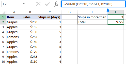
In a similar manner, you can sum values smaller than a given number. For this, use the less than ( =SUMIF(C2:C10, «
SUM IF equal to
A SUMIF formula with the «equal to» criteria works for both numbers and text. In such criteria, the equals sign is not actually required.
For instance, to find a total of the items that ship in 3 days, either of the below formulas will do:
=SUMIF(C2:C10, 3, B2:B10)
=SUMIF(C2:C10, «=3», B2:B10)
To sum if equal to cell, supply a cell reference for criteria:
=SUMIF(C2:C10, F1, B2:B10)
Where B2:B10 are the amounts, C2:C10 is the shipment duration, and F1 is the desired delivery time. 
Likewise, you can use the «equal to» criteria with text values. For instance, to add up the Apples amounts, choose any of the formulas below:
=SUMIF(A2:A10, «apples», B2:B10)
=SUMIF(A2:A10, «=apples», B2:B10)
=SUMIF(A2:A10, F1, B2:B10)
Where A2:A10 is the list of items to compare against the value in F1. 
The above formulas imply that the criterion matches the entire cell contents. Consequently, the SUMIF function will add up Apples sales but not, say, Green Apples. To sum partial matches, construct the «if cell contains» criteria like in this SUMIF wildcard formula.
Note. Please pay attention that, in Excel SUMIF formulas, a comparison or equals operator should always be enclosed in double quotes, whether used on its own or together with a number or text.
SUM IF not equal to
To build the «not equal to» criteria, use the «<>» logical operator.
When a value, either text or number, is hardcoded in the criteria, remember to surround the entire construction with double quotes.
For example, to sum the amounts with shipment other than 3 days, the formula goes as follows:
=SUMIF(C2:C10, «<>3″, B2:B10)
To find a total of all the items except Apples, the formula is:
=SUMIF(A2:A10, «<>apples», B2:B10)
When the criterion is in another cell, concatenate the «not equal to» operator and a cell reference like this:
=SUMIF(A2:A10, «<>«&F1, B2:B10) 
SUM IF blank
This example shows how to sum cells in one column if a corresponding cell in another column is blank. There are two formulas to fulfill the task. Which one to use depends on your interpretation of a «blank cell».
If «blank» means cells that contain absolutely nothing (no formula, no zero-length string returned by some other function), then use «=» for criteria. For example:
If «blank» includes empty strings (for example, cells with a formula like =»»), then use «» for criteria:
Both formulas return a total of sales for undefined regions, i.e. where a cell in column B is blank: ![]()
SUM IF not blank
To make «if cell is not blank then sum» kind of formula, use «<>» as the criteria. This will add up all cells that contain anything in them, including zero-length strings.
For instance, here’s how you can sum sales for all the regions, i.e. where column B is not blank:
=SUMIF(B2:B10, «<>«, C2:D10) ![]()
Excel SUMIF with text criteria
When adding up numbers in one column based on text values in another column, it’s important to differentiate between exact and partial match.
| Criteria | Formula Example | Description |
|---|---|---|
| Sum if equal to | Exact match: =SUMIF(A2:A8, «bananas», C2:C8) |
Sum values in cells C2:C8 if a cell in column A in the same row contains exactly the word «bananas» and no other words or characters. Cells containing «green bananas», «bananas green», or «bananas!» are not included. |
| Sum if cell contains | Partial match: =SUMIF(A2:A8, «*bananas*», C2:C8) |
Sum values in cells C2:C8 if a corresponding cell in column A contains the word «bananas», alone or in combination with any other words. Cells containing «green bananas», «bananas green», or «bananas!» are summed. |
| Sum if not equal to | Exact match: =SUMIF(A2:A8, «<>bananas», C2:C8) |
Sum values in cells C2:C8 if a cell in column A contains any value other than «bananas». If a cell contains «bananas» together with some other words or characters like «yellow bananas» or «bananas yellow», such cells are summed. |
| Sum if cell does not contain | Partial match: =SUMIF(A2:A8, «<>*bananas*», C2:C8) |
Sum values in cells C2:C8 if a cell in column A does not contain the word «bananas», alone or in combination with any other words. Cells containing «yellow bananas» or «bananas yellow» are not summed. |
For real-life formula examples, please check out Sum if equal to and Sum if not equal to.
In the next section, we’ll take a closer look at SUMIF formulas with partial match.
SUMIF formulas with wildcard characters
To conditionally sum cells by partial match, include one of the following wildcard characters in your criteria:
- Question mark (?) to match any single character in a specific position.
- Asterisk (*) to match any number of characters.
Example 1. Sum values based on partial match
Suppose you wish to total sales for all northern regions, including North, North-East, and North-West. To have it done, put an asterisk right after the word «north»:
=SUMIF(B2:B10, «north*», C2:D10)
An asterisk on both sides will also work:
=SUMIF(B2:B10, «*north*», C2:D10)
Alternatively, you can type the region of interest in a predefined cell (F1), and then concatenate a cell reference and a wildcard character enclosed in quotes:
=SUMIF(B2:B10, F1&»*», C2:D10)
=SUMIF(B2:B10, «*»&F1&»*», C2:D10) 
Example 2. Sum if cell contains * or ?
To match a literal question mark or asterisk, place a tilde (
) before the character, e.g. «
For example, to sum sales for the regions marked with *, use «*
*» for criteria. In this case, the first asterisk is a wildcard and the second one is a literal asterisk character:
If the criteria (* in our case) is entered in a separate cell, then concatenate a tilde and the cell reference, like this:
«&F1, C2:D10) 
Example 3. Sum if another cell contains text
If your dataset contains various data types and you only want to sum cells corresponding to text values, the following SUMIF formulas will come in handy.
To add up values in cells C2:C8 if a cell in column A contains any text character(s):
To sum values in C2:C8 if a cell in column A contains any text value, including zero length strings:
Both of the above formulas ignore non-text values such as numbers, dates, errors, and Booleans.
How to use Excel SUMIF with dates
Using dates as SUMIF criteria is very much like using numbers. The most important thing is to supply a date in the format that Excel understands. If you are not sure which date format is supported and which is not, the DATE function can be a solution.
Assuming you are looking to sum sales for the items delivered before 10-Sep-2020, the criteria can be expressed in this way:
Where F1 is the target date. 
To sum cells based on today’s date, include the TODAY function in your criteria. For example, that’s how you calculate a total of sales with a delivery date prior to today:
=SUMIF(C2:C10, » 
To sum within a date range, you need to define a smaller and larger date separately. This can be done with the help of the SUMIFS function that supports multiple criteria.
For example, to sum values in column B if a date in column C is between two dates, this is the formula to use:
=SUMIFS(B2:B10, C2:C10, «>=»&F1, C2:C10, «
Where B2:B10 is the sum range, C2:C10 is the list of dates to check, F1 is the start date and G1 is the end date. 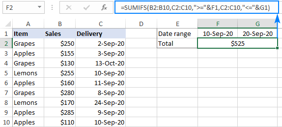
More formula examples can be found in SUMIFS with date range as criteria.
How to do SUMIF from another sheet
To conditionally sum data from a different sheet, provide external references for the SUMIF arguments. The easiest way is to start typing a formula, switch to another worksheet and select ranges using the mouse. Excel will insert all the references automatically, without you having to worry about the correct syntax.
For instance, the below formula will add up values in C2:C10 on the Data sheet based on the criteria in B3 on Sheet1:
=SUMIF(Data!B2:B10, B3, Data!C2:C10) 
How to correctly use cell references in SUMIF criteria
To create a flexible formula, you normally insert all variable parameters in predefined cells instead of «hardcoding» them. With Excel SUMIF, that might be a bit of a challenge.
In the simplest case when summing «if equal to», you simply use a cell reference for criteria. For example:
=SUMIF(C2:C10, F1, B2:B10)
But when a cell reference is used together with a logical operator, the criteria should be provided in the form of a string. So, you use the double quotes («») to start a text string and ampersand (&) to concatenate and finish the string off. For example:
=SUMIF(C2:C10, «>»&F7, B2:B10)
Please note that the comparison operators are enclosed in quotation marks while the cell references are not. 
Why is my SUMIF formula not working?
There could be several reasons why Excel SUMIF is not working for you. Sometimes, your formula does not return what you expect only because the data type in a cell or in some argument isn’t suited for the SUMIF function. Below is a list of important things to check.
1. SUMIF supports only one condition
The syntax of the SUMIF function has room for only one condition. To sum with multiple criteria, either use the SUMIFS function (adds up cells that meet all the conditions) or build a SUMIF formula with multiple OR criteria (sums cells that meet any of the conditions).
2. Range and sum_range should be of the same size
For a SUMIF formula to work correctly, the range and sum_range argument should have the same dimensions, otherwise you may get misleading results. The point is that Microsoft Excel does not rely on the user’s ability to provide matching ranges, and to avoid possible inconsistency issues, it determines the sum range automatically in this way:
Sum_range defines only the upper left cell of the range that will be summed, the remaining area is determined by the size and shape of the range argument.
Given the above, the below formula will actually sum cells in C2:C10 and not in C2:D10. Why? Because range consists of 1 column and 9 rows, and so does sum_range.
=SUMIF(B2:B10, «north», C2:D10)
In older Excel versions, unequally sized ranges can cause lots of problems. In modern Excel, complex SUMIF formulas where sum_range has less rows and/or columns than range are also capricious. That is why it’s a good practice to always define the same number of rows and columns for these two arguments.
3. Range and sum_range should be ranges, not arrays
Though SUMIF can process an array constant in criteria like shown in this example, it does not support arrays in range and sum_range. These two arguments can only be cell ranges.
5. SUMIF criteria syntax
For criteria, the SUMIF function allows using different data types including text, numbers, dates, cell references, logical operators (>, ), wildcard characters (?, *,
) and other functions. The syntax of such criteria is quite specific.
If the criteria argument includes a text value, wildcard character or logical operator followed by text, number or date, enclose the whole criteria in quotation marks. For example:
=SUMIF(B2:B10, «north*», C2:D10)
=SUMIF(B2:B10, «<>north», C2:D10)
When a logical operator is followed by a cell reference or another function, the criteria should be provided in the form of a string. So, you use an ampersand (&) to concatenate a logical operator and a reference or function. For example:
4. SUMIF from another workbook not working
As with many Excel functions, SUMIF can refer to other sheets and workbooks, provided they are currently open.
For example, this formula will work fine as long as Book1 is open:
And it will stop working as soon as Book1 is closed. This happens because the referenced ranges in closed workbooks get de-referenced into arrays. And since arrays are not supported in the range and sum_range arguments, SUMIF throws a #VALUE! error.
6. SUMIF does not recognize text case
By design, SUMIF in Excel is not case-sensitive, meaning it treats uppercase and lowercase letters as the same characters. To make a case-sensitive SUMIF formula, use the SUMPRODUCT function together with EXACT.
That’s how to use SUMIF in Excel. Hopefully, our formula examples have given you some good insights. As always, I thank you for reading and hope to see you on our blog next week!
Источник
This tutorial demonstrates how to use the Excel SUMIF and SUMIFS Functions in Excel and Google Sheets to sum data that meet certain criteria.
SUMIF Function Overview
You can use the SUMIF function in Excel to sum of cells that contain a specific value, sum cells that are greater than or equal to a value, etc.
![]()
(Notice how the formula inputs appear)
SUMIF Function Syntax and Arguments:
=SUMIF (range, criteria, [sum_range])range – The range of cells that you want to apply the criteria against.
criteria – The criteria used to determine which cells to add.
sum_range – [optional] The cells to add together. If sum_range is omitted, the cells in range are added together instead.
What is the SUMIF function?
The SUMIF function is one of the older functions used in spreadsheets. It is used to scan through a range of cells checking for a specific criterion, and then adding up values in a range that correspond to those values. The original SUMIF function was limited to just one criterion. After 2007, the SUMIFS function was created which allows a multitude of criteria. Most of the general use remains the same between the two, but there are some critical differences in the syntax that we’ll discuss throughout this article.
If you haven’t already, you can review much of the similar structure and examples in the COUNTIFS article <insert link>.
Basic example
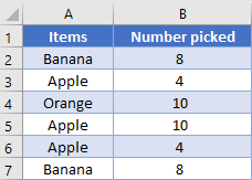
Let’s consider this list of recorded sales, and we want to know the total income.
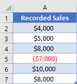
Because we had an expense, the negative value, we can’t just do a basic sum. Instead, we want to sum only the values that are greater than 0. The “greater than 0” is what will be our criteria in a SUMIF function. Our formula to state this is
=SUMIF(A2:A7, ">0")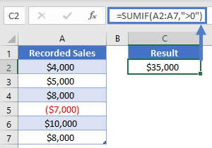
Two-column example
While the original SUMIF function was designed to let you apply a criterion to the range of numbers you want to sum, much of the time you’ll need to apply one or more criteria to other columns. Let’s consider this table:
Now, if we use the original SUMIF function to find out how many Bananas we have (listed in cell D1), we’ll need to give the range we want to sum as the last argument, and so our formula would be
=SUMIF(A2:A7, D1, B2:B7)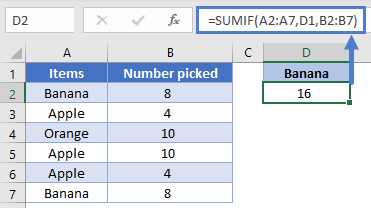
However, when programmers eventually realized that users wanted to give more than one criterion, the SUMIFS function was created. In order to create one structure that would work for any number of criteria, the SUMIFS requires that the sum range is listed first. In our example, this means that the formula needs to be
=SUMIFS(B2:B7, A2:A7, D1)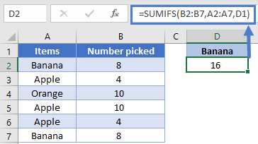
NOTE: These two formulas get the same result and can look similar, so pay close attention to which function is being used to make sure you list out all the arguments in the correct order.
Working with Dates, Multiple criteria
When working with dates in a spreadsheet, while it is possible to input the date directly into the formula, it’s best practice to have the date in a cell so that you can just reference the cell in a formula. For example, this helps the computer know that you’re wanting to use the date 5/27/2020, and not the number 5 divided by 27 divided by 2020.
Let’s look at our next table recording the number of visitors to a site every two weeks.
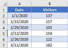
We can specify the start and end points of the range we want to look at in D2 and E2. Our formula then to sum the number of visitors in this range could be:
=SUMIFS(B2:B7, A2:A7, ">="&D2, A2:A7, "<="&E2)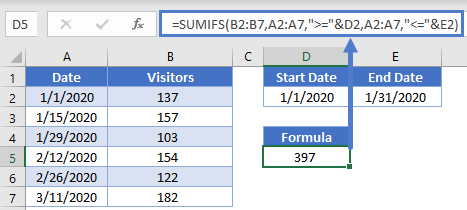
Note how we were able to concatenate the comparisons of “<=” and “>=” to the cell references to create the criteria. Also, even though both criteria were being applied to the same range of cells (A2:A7), you need to write out the range twice, once per each criterion.
Multiple columns
When using multiple criteria, you can apply them to the same range as we did with previous example, or you can apply them to different ranges. Let’s combine our sample data into this table:
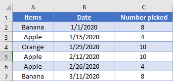
We’ve setup some cells for the user to enter what they want to search for in cells E2 through G2. We thus need a formula that will add up the total number of apples picked in February. Our formula looks like this:
=SUMIFS(C2:C7, B2:B7, ">="&F2, B2:B7, "<="&G2, A2:A7, E2)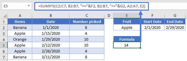
SUMIFS with OR type logic
Up to this point, the examples we’ve used have all been AND based comparison, where we are looking for rows that meet all our criteria. Now, we’ll consider the case when you want to search for the possibility of a row meeting one or another criterion.
Let’s look at this list of sales:
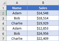
We’d like to add up the total sales for both Adam and Bob. To do this, you have a couple of options. The simplest is to add two SUMIFS together, like so:
=SUMIFS(B2:B7, A2:A7, "Adam")+SUMIFS(B2:B7, A2:A7, "Bob")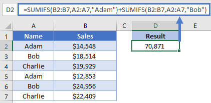
Here, we’ve had the computer calculate our individual scores, and then we add them together.
Our next option is good for when you have more criteria ranges, such that you don’t want to have to rewrite the whole formula repeatedly. In the previous formula, we manually told the computer to add two different SUMIFS together. However, you can also do this by writing your criteria inside an array, like this:
=SUM(SUMIFS(B2:B7, A2:A7, {"Adam", "Bob"}))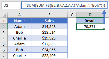
Look at how the array is constructed inside the curly brackets. When the computer evaluates this formula, it will know that we want to calculate a SUMIFS function for each item in our array, thus creating an array of numbers. The outer SUM function will then take that array of numbers and turn it into a single number. Stepping through the formula evaluation, it would look like this:
=SUM(SUMIFS(B2:B7, A2:A7, {"Adam", "Bob"}))
=SUM(27401, 43470)
=70871
We get the same result, but we were able to write out the formula a bit more succinctly.
Dealing with blanks
Sometimes your data set will have blank cells that you need to either find or avoid. Setting up the criteria for these can be a little tricky, so let’s look at another example.
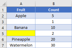
Note that cell A3 is truly blank, while cell A5 has a formula returning a zero-length string of “”. If we want to find the total sum of truly blank cells, we’d use a criterion of “=”, and our formula would look like this:
=SUMIFS(B2:B7,A2:A7,"=")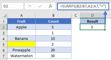
On the other hand, if we want to get the sum for all cells that visually looks blank, we’ll change the criteria to be “”, and the formula looks like
=SUMIFS(B2:B7,A2:A7,"")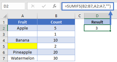
Let’s flip it around: what if you want to find the sum of non-blank cells? Unfortunately, the current design won’t let you avoid the zero-length string. You can use a criterion of “<>”, but as you can see in the example, it still includes the value from row 5.
=SUMIFS(B2:B7,A2:A7,"<>")
If you need to not count cells containing zero length strings, you’ll want to consider using the LEN function inside a SUMPRODUCT <link to SUMPRODUCT article).
SUMIF in Google Sheets
The SUMIF Function works exactly the same in Google Sheets as in Excel:
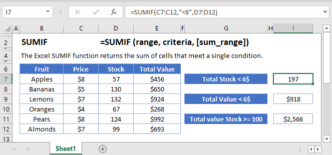
The SUMIF function sums cells in a range that meet a single condition, referred to as criteria. The SUMIF function is a common, widely used function in Excel, and can be used to sum cells based on dates, text values, and numbers. Note that SUMIF can only apply one condition. To sum cells using multiple criteria, see the SUMIFS function.
Syntax
The generic syntax for SUMIF looks like this:
=SUMIF(range,criteria,[sum_range])The SUMIF function takes three arguments. The first argument, range, is the range of cells to apply criteria to. The second argument, criteria, is the criteria to apply, along with any logical operators. The last argument, sum_range, is the range that should be summed. Note that sum_range is optional. If sum_range is not provided, SUMIF will sum cells in the first argument, range.
Examples: Basic Usage | Criteria in another cell | Not equal to | Blank cells | Dates | Wildcards | Videos
Applying criteria
The SUMIF function supports logical operators (>,<,<>,=) and wildcards (*,?) for partial matching. The tricky part about using the SUMIF function is the syntax needed to apply criteria. This is because SUMIF is in a group of eight functions that split logical criteria into two parts, range and criteria. Because of this design, operators need to be enclosed in double quotes («»). The table below shows examples of the syntax needed for common criteria:
| Target | Criteria |
|---|---|
| Cells greater than 75 | «>75» |
| Cells equal to 100 | 100 or «100» |
| Cells less than or equal to 100 | «<=100» |
| Cells equal to «Red» | «red» |
| Cells not equal to «Red» | «<>red» |
| Cells that are blank «» | «» |
| Cells that are not blank | «<>» |
| Cells that begin with «X» | «x*» |
| Cells less than A1 | «<«&A1 |
| Cells less than today | «<«&TODAY() |
Notice the last two examples involve concatenation with the ampersand (&) character. Any time you are using a value from another cell, or using the result of a formula in criteria with a logical operator like «<«, you will need to concatenate. This is because Excel needs to evaluate cell references and formulas to get a value before that value can be joined with an operator.
Limitations
There are a couple of limitations with SUMIF that you should be aware of. First, SUMIF only supports a single condition. If you need to sum cells using multiple criteria, use the SUMIFS function. Second, the SUMIF function requires an actual range for the range argument; you can’t substitute an array. This means you can’t do things like extract the year from a range that contains dates inside the SUMIF function. If you need to manipulate values that appear in the argument before applying criteria, the SUMPRODUCT function is a flexible solution.
Basic usage
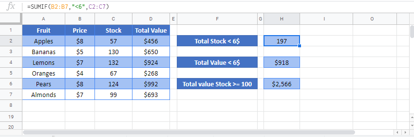
With numbers in the range A1:A10, you can use SUMIF to sum cells greater than 5 like this:
=SUMIF(A1:A10,">5")If the range B1:B10 contains color names like «red», «blue», and «green», you can use SUMIF to sum numbers in A1:A10 when the color in B1:B10 is «red» like this:
=SUMIF(B1:B10,"red",A1:A10)Notice A1:A10 is now entered as the sum_range, because it is different from range, which contains only color names. To recap: criteria is applied to cells in range. When cells in range meet criteria, corresponding cells in sum_range are summed. The sum_range argument is optional. If sum_range is omitted, the cells in range are summed instead.
Worksheet example
In the worksheet shown, there are three SUMIF formulas. In the first formula (G5), SUMIF returns total Sales where Name = «jim». In the second formula (G6), SUMIF returns total Sales where State = «ca» (California). In the third formula (G7), SUMIF returns the total of Sales > 100:
=SUMIF(B5:B15,"jim",D5:D15) // name = "jim"
=SUMIF(C5:C15,"ca",D5:D15) // state = "ca"
=SUMIF(D5:D15,">100") // sales > 100
Notice the equals sign (=) is not required when constructing «is equal to» criteria. Also notice SUMIF is not case-sensitive; you can use «jim» or «Jim». Finally, notice that the last formula does not include sum_range, so range is summed instead.
Criteria in another cell
A value from another cell can be included in criteria using concatenation. In the example below, SUMIF will return the sum of all sales over the value in G4. Notice the greater than operator (>), which is text, must be enclosed in quotes. The formula in G5 is:
=SUMIF(D5:D9,">"&G4) // sum if greater than G4

Not equal to
To express «not equal to» criteria, use the «<>» operator surrounded by double quotes («»):

=SUMIF(B5:B9,"<>red",C5:C9) // not equal to "red"
=SUMIF(B5:B9,"<>blue",C5:C9) // not equal to "blue"
=SUMIF(B5:B9,"<>"&E7,C5:C9) // not equal to E7
Again notice SUMIF is not case-sensitive.
Blank cells
SUMIF can calculate sums based on cells that are blank or not blank. In the example below, SUMIF is used to sum the amounts in column C depending on whether column D contains «x» or is empty:

=SUMIF(D5:D9,"",C5:C9) // blank
=SUMIF(D5:D9,"<>",C5:C9) // not blank
Dates
The best way to use SUMIF with dates is to refer to a valid date in another cell, or use the DATE function. The example below shows both methods:

=SUMIF(B5:B9,"<"&DATE(2019,3,1),C5:C9)
=SUMIF(B5:B9,">="&DATE(2019,4,1),C5:C9)
=SUMIF(B5:B9,">"&E9,C5:C9)
Notice we must concatenate an operator to the date in E9. To use more advanced date criteria (i.e. all dates in a given month, or all dates between two dates) you’ll want to switch to the SUMIFS function, which can handle multiple criteria.
Wildcards
The SUMIF function supports wildcards, as seen in the example below:

=SUMIF(B5:B9,"mi*",C5:C9) // begins with "mi"
=SUMIF(B5:B9,"*ota",C5:C9) // ends with "ota"
=SUMIF(B5:B9,"????",C5:C9) // contains 4 characters
The tilde (~) is an escape character to allow you to find literal wildcards. For example, to match a literal question mark (?), asterisk(*), or tilde (~), add a tilde in front of the wildcard (i.e. ~?, ~*, ~~).
Average range caution
SUMIF makes certain assumptions about the size of sum_range, essentially resizing it when necessary to match the range argument, using the upper left cell in the range as an origin. In some cases, this behavior can create a result that seems reasonable but is in fact incorrect. For an example of this problem, see this article.
Notes
- SUMIF only supports one condition. Use the SUMIFS function for multiple criteria.
- When sum_range is omitted, the cells in range will be summed.
- Non-numeric criteria must be enclosed in double quotes (i.e. «<100», «>32», «TX»)
- Cell references in criteria are not enclosed in quotes, i.e. «<«&A1
- The wildcard characters ? and * can be used in criteria. A question mark matches any one character and an asterisk matches any sequence of characters (zero or more).
- To match a literal question mark(?) or asterisk (*), use a tilde (~) like (~?, ~*).
- SUMIF requires a range, you can’t substitute an array.