If and subtotal excel

This tutorial will demonstrate how to calculate the “subtotal if”, performing the SUBTOTAL Function, only on cells that meet certain criteria.

SUBTOTAL Function

The SUBTOTAL Function is used to perform various calculations on a range of data (count, sum, average, etc.). If you’re not familiar with the function, you might be wondering why you wouldn’t just use the COUNT, SUM, or AVERAGE Functions themselves…  There are two good reasons:

1. You could create a table that lists the SUBTOTAL Options (1,2,3,4, etc.) and copy a single formula down to create summary data. (This could be an especially big time-saver if you’re attempting to calculate SUBTOTAL IF as we demonstrate in this article).
2. The SUBTOTAL Function can be used to calculate only visible (filtered) rows.

We will focus on the second implementation of the SUBTOTAL Function.

In this example, we will be using the function to count (COUNTA) visible rows by setting the SUBTOTAL function_num argument to 3 (A full list of possible functions can be found here.)

=SUBTOTAL(3,$D$2:$D$14)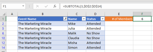

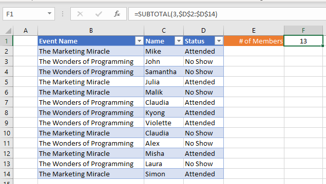
Notice how the results change as we manually filter rows.

SUBTOTAL IF

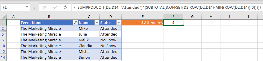
To create a “Subtotal If”, we will use a combination of SUMPRODUCT, SUBTOTAL, OFFSET, ROW, and MIN in an array formula. Using this combination, we can essentially create a generic “SUBTOTAL IF” function. Let’s walk through an example.

We have a list of members and their attendance status for each event:

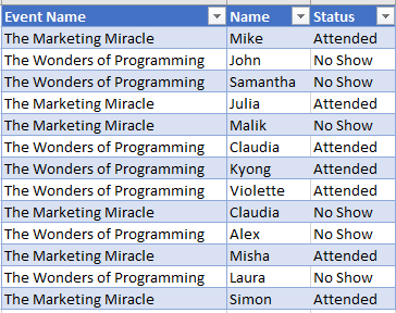
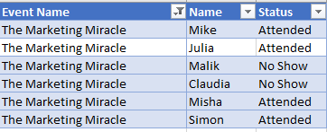
Supposed we are asked to count the number of members that have attended an event dynamically as we manually filter the list like so:

To accomplish this, we can use this formula:

=SUMPRODUCT((<values range>=<criteria>)*(SUBTOTAL(3,OFFSET(<first cell in range>,ROW(<values range>)-MIN(ROW(<values range>)),0))))

=SUMPRODUCT((D2:D14="Attended")*(SUBTOTAL(3,OFFSET(D2,ROW(D2:D14)-MIN(ROW(D2:D14)),0))))

When using Excel 2019 and earlier, you must enter the array formula by pressing CTRL + SHIFT + ENTER to tell Excel that you’re entering an array formula. You’ll know the formula was entered properly as an array formula when curly brackets appear around the formula (see image above).

How does the formula work?

The formula works by multiplying two arrays inside of SUMPRODUCT, where the first array deals with our criteria and the second array filters to visible rows only:

=SUMPRODUCT(<criteria array>*<visibility array>)

The Criteria Array

The criteria array evaluates each row in our values range (“Attended” Status in this example) and generates an array like this:

=(<values range>=<criteria>)

=(D2:D14="Attended")

Output:

{TRUE; FALSE; FALSE; TRUE; FALSE; TURE; TURE; TURE; FALSE; FALSE; TRUE; FALSE; TRUE}

Note that the output in the first array in our formula ignore whether the row is visible or not, which is where our second array comes in to help.

The Visibility Array

Using SUBTOTAL to exclude non-visible rows in our range, we can generate our visibility array. However, SUBTOTAL alone will return a single value, while SUMPRODUCT is expecting an array of values. To work around this, we use OFFSET to pass one row at a time. This technique requires feeding OFFSET an array that contains one number at time. The second array looks like this:

=SUBTOTAL(3,OFFSET(<first cell in range>,ROW(<values range>)-MIN(ROW(<values range>)),0))

=SUBTOTAL(3,OFFSET(D2,ROW(D2:D14)-MIN(ROW(D2:D14)),0))

Output:

{1;1;0;0;1;1}

Stitching the two together:

=SUMPRODUCT({TRUE; TRUE; FALSE; FALSE; TRUE; TRUE} * {1; 1; 0; 0; 1; 1})

= 4

SUBTOTAL IF with Multiple Criteria

To add multiple criteria, simply multiple more criteria together within the SUMPRODUCT like so:

=SUMPRODUCT((<values range 1>=<criteria 1>)*(<values range 2>=<criteria 2>)*(SUBTOTAL(3,OFFSET(<first cell in range>,ROW(<values range>)-MIN(ROW(<values range>)),0))))

=SUMPRODUCT((E2:E14="Attended")*(B2:B14=2019)*(SUBTOTAL(3,OFFSET(E2,ROW(E2:E14)-MIN(ROW(E2:E14)),0))))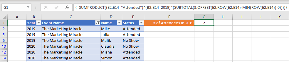

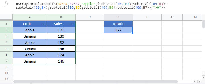
SUBTOTAL IF in Google Sheets

The SUBTOTAL IF Function works exactly the same in Google Sheets as in Excel. Except that notice when you use CTRL + SHIFT + ENTER to enter the array formula, Google Sheets adds the function ARRAYFORMULA to the formula (you can also manually add this function).

• #2

try this:

=if(subtotal(A1:A12=whatever,»»,(subtotal(A1:A12)

something like that although i havent used subtotal before so you may need to adjust it

HTH

• #3

Can you insert a column and use an IF statement in that column and then use that column for your subtotals?

• #4

The criteria is in an another column. I need a formula that solves:
«Subtotal range C2:C50 if range B2:B50 is >0». I want to use the SUMIF logic but with filtering flexibility of the SUBTOTAL function.
BuzzG

• #5

post your current formula here

• #6

BuzzG said:

The criteria is in an another column. I need a formula that solves:
«Subtotal range C2:C50 if range B2:B50 is >0». I want to use the SUMIF logic but with filtering flexibility of the SUBTOTAL function.
BuzzG

Insert a column and put this in row 2
=IF(B2>0,C2,0)

Copy this down to row 50 and then use your subtotal on that column. Excel does not have a SUMIF capability in conjunction with SUBTOTAL.

Best regards,

• #7

Barrie is it not possible to use something like this:

=if(subtotal(A1:A12=whatever,»»,(subtotal(A1:A12)

this in theory gives you a subtotalIF

• #8

Barrie’s solution will work. I was just hoping for a fancy SUBTOTALIF solution from Microsoft.
Thanks for your help
BuzzG

• #9

BuzzG said:

The criteria is in an another column. I need a formula that solves:
«Subtotal range C2:C50 if range B2:B50 is >0». I want to use the SUMIF logic but with filtering flexibility of the SUBTOTAL function.
BuzzG

=SUMPRODUCT(SUBTOTAL(3,OFFSET(C2:C50,ROW(C2:C50)-MIN(ROW(C2:C50)),,1)),—(B2:B50>0),C2:C50)

• #10

I am using this formula and trying to get to do one more thing:

=SUMPRODUCT(SUBTOTAL(3,OFFSET(F14:F61,ROW(F14:F61)-MIN(ROW(F14:F61)),,1)),—(J14:J61=»Facility Design»),F14:F61)

I want to subtotal F14:F61 only if it equals 100% and has «Facility Design» in another column. I have tried different things but am rather new to the world of formulas.

I dont even know if I need such a complex formula for my needs. I just to total the 100% in a column only if another column has «blah blah».

Any insight would be great. Thanks.

Without using any helper column, we can use the Subtotal function with conditions in Excel and Google Sheets in a filtered dataset.

Here is a new Excel vs. Google Sheets formula comparison.

It is not a function comparison between Excel and Google Sheets but a formula comparison.

In this particular formula comparison that involves a combination formula, I see the Excel formula is better than the formula in Google Sheets.

Sheets require the help of Lambda to spill results, whereas Excel doesn’t need it.

We cannot exclude filtered out or hidden rows in conditional functions like Countif, Sumif, Minifs, Maxifs, and Averageif in Google Sheets and Excel.

The only function that works on filtered data is Subtotal. It works equally well on data that is hidden. So we must make use of it in all possible ways.

Introduction to Subtotal Function in Excel and Google Sheets

The Subtotal is a versatile function that subtotals a range with specific functions.

That specific function list includes the below functions and represents them in Subtotal with function numbers.

Function Code/Number in Subtotal in Excel and Google Sheets are the same.

Function # Excludes Filtered Out Rows	Function # Excludes All Hidden Rows
AVERAGE 1	AVERAGE 101
COUNT 2	COUNT 102
COUNTA 3	COUNTA 103
MAX 4	MAX 104
MIN 5	MIN 105
PRODUCT 6	PRODUCT 106
STDEV 7	STDEV 107
STDEVP 8	STDEVP 108
SUM 9	SUM 109
VAR 10	VAR 110
VARP 11	VARP 111

In the below examples, I am using some of the function numbers from the above list.

Comparison to the Use of Subtotal Function With Conditions in Excel and Google Sheets

First, let me share with you how to use Subtotal to count, sum, min, max, and average in Excel and as well as in Google Sheets.

Then you can learn how to use conditions in the Subtotal function in Excel and Google Sheets.

The function Subtotal works similarly in Excel and Google Sheets. The below formula examples work in both the said two popular Spreadsheet applications.

Screen Capture # 1 from Excel:

I have only included a few aggregate functions in the above Subtotal formulas. The reason I am detailing the use of conditions only in those functions.

Just filter the data or hide rows to see the formula results vary as the Subtotal formulas present above only aggregate the values in the visible rows.

Criteria in Subtotal in Excel and Google Sheets – Helper Column Approach

Conditions/Criteria in Subtotal reminds me of the possibility of a new SubtotalIf function.

But unfortunately, at present, there is no such function in Excel or Google Sheets. Let me come to the point.

How to prepare a helper column for Subtotal If or you can say to use conditions in Subtotal?

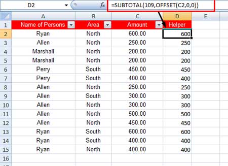
Screen Capture # 2 from Excel:

In my above example, column D is my helper column.

In that column, apply the below Subtotal formula in cell D2 and drag it down to fill until cell D15.

=SUBTOTAL(109,C2)

Note:- Use =SUBTOTAL(103,C2) if column C is text type, not numeric.

To test the purpose of the above helper column, in cell F2 key in the following formula.

=D5

It will return the value 200, which is the value in cell D5, right?

Now select row # 5, right-click, and from the shortcut menu, select Hide to hide the row.

You can see that the formula in cell F2 now returns 0!

That means when you hide any row, the value in column D in that row will be 0.

It will help you conditionally aggregate values in column C.

I’ll explain how. Before that, you must see how I am aggregating columns without the function Subtotal and excluding hidden/filter rows in Excel and Google Sheets.

Yes, once you have a helper column as above, you can use aggregate functions in Google Sheets and Excel without the Subtotal and aggregate function numbers.

Below is the replacement of the Subtotal formulas provided in the first screenshot, except for counta.

Further, below each of them, you can see one additional formula as an example of the Subtotal function with conditions in Excel and Google Sheets.

Averageif Visible Rows in Excel and Google Sheets

Formula:

=AVERAGEIF(D2:D15,">0",C2:C15)

This formula would return the average value of the numbers in the range C2:C15 but for only the visible rows.

Take a look at the first screenshot. There you can see the Subtotal formula with function # 101. It’s equivalent to that.

Now let us see how to include conditions in Subtotal. See the below Subtotal If Formula equivalent that contains criterion/condition.

=AVERAGEIFS(C2:C15,D2:D15,">0",A2:A15,"Ryan")

The above two and the following formulas work in Excel and Google Sheets. Both formulas calculate averages in different ways.

While the first formula finds the average of the visible rows, the second formula further checks whether the given criterion matches column A.

Countif Visible Rows in Excel and Google Sheets

Formula:

=COUNTIF(D2:D15,">0")

The Subtotal If Formula (Equivalent) with Conditions:

=COUNTIFS(D2:D15,">0",A2:A15,"Ryan")

This formula counts the name “Ryan” but only the visible names.

Please refer to my Google Sheets Functions Guide if you have any queries regarding any of the functions mentioned in this tutorial.

Minifs Visible Rows in Excel and Google Sheets

Formula:

=MINIFS(C2:C15,D2:D15,">0")

The Subtotal If Formula (Equivalent) with Conditions:

=MINIFS(C2:C15,D2:D15,">0",A2:A15,"Ryan")

This formula is an example of the use of Minifs in Google Sheets and Excel, excluding hidden or filtered-out rows.

It returns the min of visible rows for the names in column A, i.e., “Ryan.”

Maxifs Visible Rows in Excel and Google Sheets

Formula:

=MAXIFS(C2:C15,D2:D15,">0")

It follows the same Minifs approach in visible rows.

=MAXIFS(C2:C15,D2:D15,">0",A2:A15,"Ryan")

Sumif Visible Rows in Excel and Google Sheets

Formula:

=SUMIF(D2:D15,">0",C2:C15)

The Subtotal Formula Alternative with Conditions:

=SUMIFS(C2:C15,D2:D15,">0",A2:A15,"Ryan")

Sumif and Sumifs are two popular worksheet functions similar to Vlookup.

Sumif/Sumifs, by default, can’t conditionally sum visible rows. 

The above helper column approach helps to achieve that in Excel and Google Sheets.

Conditions in Subtotal in Excel Without Helper Column (Non-Lambda Approaches)

The below formula would only work in Excel. Even if you find it works in Google Sheets without any visible formula parse error, that output may not be correct.

We can use the Subtotal function with conditions/criteria in Excel without any helper column.

In Excel, we can generate the above helper column with the help of offset rows.

You can understand one thing if you scroll up and see the formulas in the helper column.

In each cell, there is a subtotal formula. The same we can generate virtually using the below one-line piece of code.

=SUBTOTAL(109,OFFSET(C2,ROW(C2:C15)-ROW(C2),0)

Can you explain the logic?

Yes! It’s just like entering the below formula in helper column cell D2 and then dragging it down.

=SUBTOTAL(109,OFFSET(C2,0,0))

Screen Capture # 3 from Excel:

In Excel, we can turn this offset formula into an Array Formula by using Sumproduct or the Ctrl+Shift+Enter legacy array method depending on the version of Excel you use.

The Ctrl+Shift+Enter may not be required in Excel 365.

So the helper column is not required in Excel. That means the Subtotal function with conditions in Excel doesn’t require a helper column.

Formula Examples to Criteria Usage in Subtotal in Excel Without Helper Column

To sum visible rows with conditions in another column, or you can say Sumif Visible Rows with Criteria in Excel, you can use my below formula.

Formula:

=SUMPRODUCT((A2:A15="Marshall")*(SUBTOTAL(109,OFFSET(C2,ROW(C2:C15)-ROW(C2),0))))

It doesn’t use any helper column.

The following formula counts visible rows with conditions in another column.

The Formula to Countif Visible Rows with Criteria in Excel:

=SUMPRODUCT((A2:A15="Marshall")*(SUBTOTAL(103,OFFSET(C2,ROW(C2:C15)-ROW(C2),0))))

You can use the following Excel formula to find the max value in a column in the visible rows based on conditions in another column.

It must be entered as an Array Formula using Ctrl+Shift+Enter since there is no Sumproduct with it.

The Formula to Maxifs Visible Rows with Condition in Excel:

=MAX(IF(A2:A15="Marshall",SUBTOTAL(109,OFFSET(C2,ROW(C2:C15)-ROW(C2),0)),""))

The below formula must also be entered as Array Formula using Ctrl+Shift+Enter.

Screen Capture # 4 from Excel:

Minifs Visible Rows with Criteria in Excel:

=MIN(IF(A2:A15="Marshall",SUBTOTAL(109,OFFSET(C2,ROW(C2:C15)-ROW(C2),0)),""))

Averageif Visible Rows with Criteria in Excel:

You must enter this formula as an array formula.

It finds the average of visible rows without a helper column. Also, it checks the condition in another column.

=AVERAGE(IF(A2:A15="Marshall",IF(SUBTOTAL(109,OFFSET(C2,ROW(C2:C15)-ROW(C2),0,1))>0,C2:C15)))

In the last five formulas, treat the first two as regular formulas.

The last three formulas must be entered as array formulas.

There are only slight differences in the formulas. The logic of offset rows in subtotal is the same in all five.

New Changes Both in Excel and Google Sheets (Non-Helper Lambda Approaches)

A lot of water has flown under the bridge. Now it’s easy to use Subtotal with conditions in Excel and Google Sheets without a helper column.

All thanks go to the Lambda helper functions. Here is an example.

You May Like: SUMIF Excluding Hidden Rows in Google Sheets [Without Helper Column].

The same approach will work in Excel also.

That’s all about how to use the Subtotal function with conditions in Excel and Google Sheets. I hope you have enjoyed your stay!

Microsoft Excel, Microsoft Office

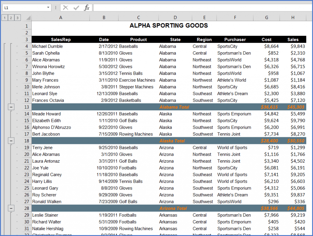
If there has ever been a more “You’ve got your chocolate in my peanut butter!” moment, it’s the blending of Conditional Formatting with the Subtotals tool in Excel.

If you have ever used the Subtotals tool to group information you have probable been impressed with its ability to group data by some changing event (like States) and have those groups aggregated and then structured into a collapsible outline.

Before Subtotals

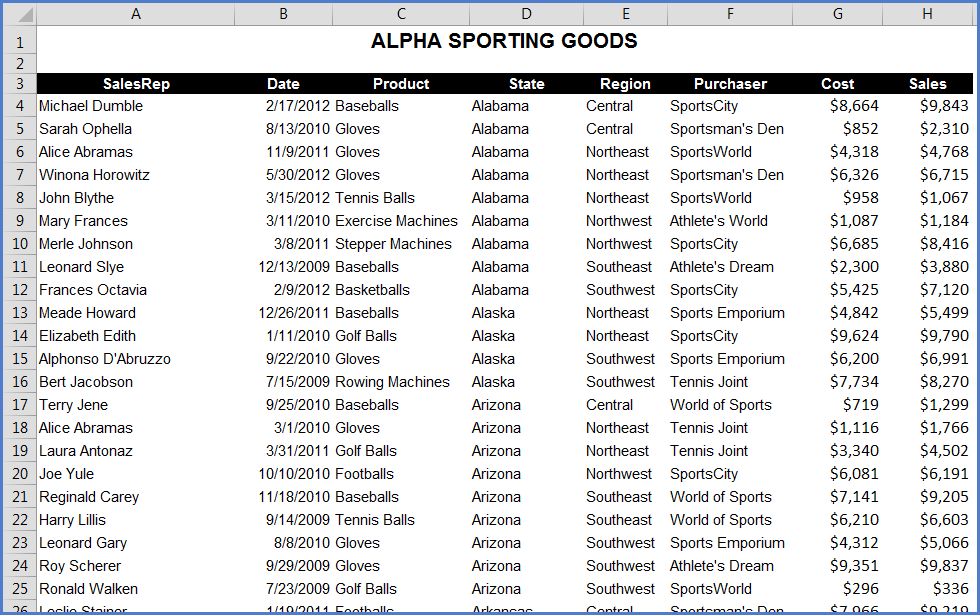
After Subtotals

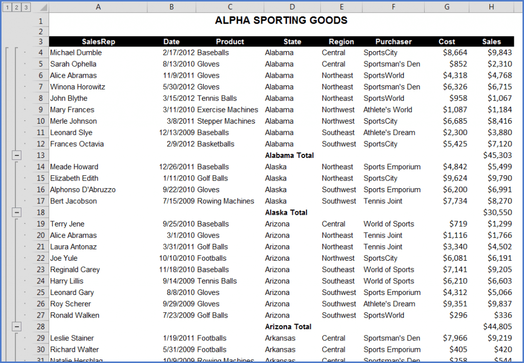
But the one shortfall when it comes to the Subtotals tool is that there are no built-in artistic styles that can be applied to give the list a bit of pizazz.

You could try to convert the list to a Data Table, but that tool is really meant for straight tables with no intermediate calculations.

CONDITIONAL FORMATTING TO THE RESCUE!!!!!!!!!!!

A common request among Excel users is to have the Subtotal lines be filled with a color to help identify them with greater ease.   Conditional Formatting is so versatile when painting data based on some criteria, it becomes a perfect tool for achieving just the desired look.  Here are the steps:

Step 1:  Selecting the Data Range

Highlight all of the columns containing data.  In the above example, that would be Columns “A” through “H” (A:H).  This is a good strategy when you are unsure as to the number of records contained in the data.  If you wish to be a bit more conservative with memory management, select a range of cells that you are sure you will never exceed (i.e. A4:H1000).

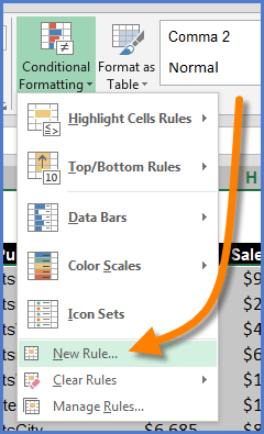
Step 2:  Create a New Conditional Format Based on a Formula

On the Home tab, click the Conditional Formatting button and select New Rule…

The formula needed to achieve the highlight effect is as follows:

=ISNUMBER(SEARCH(“Total”,$D1))

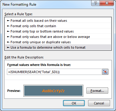
The purpose of this formula is to search for the word “Total” in the text contained in Column “D”.  If it finds the word “Total”, it will return the character position of the word within the text (i.e. “9” in the case of “Alabama Total”).

The ISNUMBER function then checks to see if a number was discovered (the word “Total” exists) or an error was returned (“#VALUE” if the word “Total” was not found).  This generates a “True/False” response that is passed to the Conditional Formatting tool.

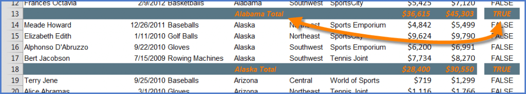
Since every cell in the selected range is looking at its Column “D” position, every cell on a row containing the word “Total” will receive the new formatting instruction.

Step 3:  Apply Color Scheme

This step is all about making the cell the color(s) that looks best for the report and the tastes of the designer and viewer.