If and statement excel with dates - Word и Excel - помощь в работе с программами

The IF function is one of the most useful Excel functions. It is used to test a condition and return one value if the condition is TRUE and another if it is FALSE.

One of the most common applications of the IF function involves the comparison of values.

These values can be numbers, text, or even dates. However, using the IF statement with date values is not as intuitive as it may seem.

In this tutorial, I will demonstrate some ways in which you can use the IF function with date values.

Syntax and Usage of the IF Function in Excel

The syntax for the IF function is as follows:

IF(logical_test, [value_if_true], [value_if_false])

Here,

logical_test is the condition or criteria that you want the IF function to test. The result of this parameter is either TRUE or FALSE
value_if_true is the value that you want the IF function to return if the logical_test evaluates to TRUE
value_if_false is the value that you want the IF function to return if the logical_test evaluates to FALSE

For example, say you want to write a statement that will return the value “yes” if the value in cell reference A2 is equal to 10, and “no” if it’s anything but 10.

You can then use the following IF function for this scenario:

=IF(A2=10,"yes","no")

Comparing Dates in Excel (Using Operators)

Unlike numbers and strings, comparison operators, when used with dates, have a slightly different meaning.

Here are some of the comparison operators that you can use when comparing dates, along with what they mean:

Operator	What it Means When Using with Dates
<	Before the given date
=	Same as the date with which we are comparing
>	After the given date
<=	Same as or before the given date
>=	Same as or after the given date

It may look like IF formulas for dates are the same as IF functions for numeric or text values, since they use the same comparison operators.

However, it’s not as simple as that.

Unfortunately, unlike other Excel functions, the IF function cannot recognize dates.

It interprets them as regular text values.

So you cannot use a logical test such as “>05/07/2021” in your IF function, as it will simply see the value “05/07/2021” as text.

Here are a few ways in which you can incorporate date values into your IF function’s logical_test parameter.

Using the IF Function with DATEVALUE Function

If you want to use a date in your IF function’s logical test, you can wrap the date in the DATEVALUE function.

This function converts a date in text format to a serial number that Excel can recognize as a date.

If you put a date within quotes, it is essentially a text or string value.

When you pass this as a parameter to the DATEVALUE function, it takes a look at the text inside the double quotes, identifies it as a date and then converts it to an actual Excel date value.

Let us say you have a date in cell A2, and you want cell B2 to display the value “done” if the date comes before or on the same date as “05/07/2021” and display “not done” otherwise.

You can use the IF function along with DATEVALUE in cell B2 as follows:

=IF(A2<DATEVALUE("05/07/2021"),"done","not done")

Here’s a screenshot to illustrate the effect of the above formula:

Using the IF Function with the TODAY Function

If you want to compare a date with the current date, you can use the IF function with the TODAY function in the logical test.

Let’s say you have a date in cell A2 and you want cell B2 to display the value “done” if it is a date before today’s date.

If not, you want let’s say you want to display the value “not done”. You can use the IF function along with the TODAY function in cell B2 as follows:

=IF(A2<TODAY(),"done","not done")

Here’s a screenshot to illustrate the effect of the above formula (assuming the current date is 05/08/2021):

IF Formula to check whether date is before today

Using the IF Function with Future or Past Dates

An interesting thing about dates in Excel is that you can perform addition and subtraction operations with them too.

This is because dates are basically stored in Excel as serial numbers, starting from the date Jan 1, 1900.

Each day after that is represented by one whole number.

So, the serial number 2 corresponds to Jan 2, 1900, and so on.

This means that adding n number of days to a date is equivalent to adding the value n to the serial number that the date represents.

If TODAY() is 05/07/2021, then TODAY()+5 is five days after today, or 05/12/2021. Similarly, TODAY()-3 is three days before today or 05/04/2021.

Let’s say you have a date in cell A2 and you want cell B2 to mark it as “within range” if it is within 15 days from the current date.

If not, you want to show “out of range”. You can use the IF function along with the TODAY function in cell B2 as follows:

=IF(A2<TODAY()+15,"within range","out of range")

Here’s a screenshot to illustrate the effect of the above formula (assuming the current date is 05/08/2021):

IF formula to check whether date is within range

Points to Remember

Having discussed different ways to use dates with the IF function, here are some important points to remember:

Instead of hardcoding the dates into the IF function’s logical test parameter, you can store the date in a separate cell and refer to it with a cell reference. For example, instead of typing =IF(A2<”05/07/2021”,”done”,”not done”), you can store the date 05/07/2021 in a cell, say B2 and type the formula: =IF(A2<B2,”done”,”not done”).

Alternatively, you can use the DATEVALUE function as explained in the first part of this tutorial.

Another neat technique that you can use is to simply add a zero to the date (which has been enclosed in double quotes). So you can type: =IF(A2<”05/07/2021”+0,”done”,”not done”). This will make Excel take the date inside double quotes as a serial number, and use it in the logical test without having its value changed.

In this tutorial, I showed you some great techniques to use the IF function with dates. I hope the tips covered here were useful for you.

Other articles you may also like:

Multiple If Statements in Excel (Nested Ifs, AND/OR) with Examples
How to use Excel If Statement with Multiple Conditions Range [AND/OR]
How to Convert Month Number to Month Name in Excel
Why are Dates Shown as Hashtags in Excel? Easy Fix!
How to Convert Serial Numbers to Date in Excel
How to Get the First Day Of The Month In Excel?

Источник

If you have a list of dates and then want to compare to these dates with a specified date to check if those dates is greater than or less than that specified date. You can use the IF function in combination with logical operators and DATEVALUE function in Microsoft excel.

Table of Contents

Excel IF function combining with DATEVALUE function
Excel IF function combining with DATE function
Excel IF function combining with TODAY function
- Related Formulas
- Related Functions

Excel IF function combining with DATEVALUE function

Since that Excel cannot recognize the date formats and just interprets them as a text string. So you need to use DATAVALUE function and let Excel think that it is a Date value. For example: DATEVALUE(“11/3/2018”). Now we can write down the following IF formula with Dates.

=IF(B1<DATEVALUE(“11/3/2018”),”good”,”bad”)

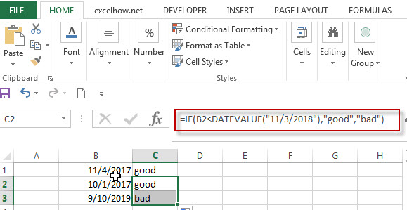
The above excel IF formula will check the date value in Cell B1 if it is less than another specified date(11/3/2018), if the test is TRUE, then return “good”, otherwise return “bad”

Excel IF function combining with DATE function

You can also use DATE function in an Excel IF statement to compare dates, like the below IF formula:

=IF(B1<=DATE(2018,11,3),”good”,””)

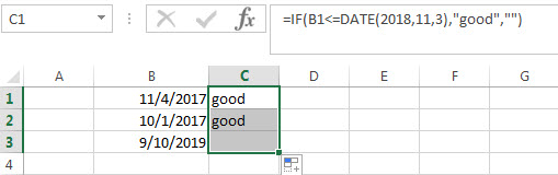
The above IF formula will check if the value in cell B1 is less than or equal to 11/3/2018 and show the returned value in cell C1, Otherwise show nothing.

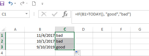
Excel IF function combining with TODAY function

If you want to compare the current date with the specified date in the past, you can use IF function in combination with TODAY function in Excel. Like the following IF formula:

=IF(B1>TODAY(), “good”,”bad”)

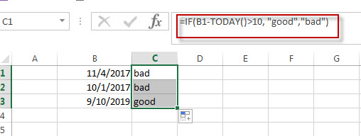
We also can use the complex logical test using Today function, like this: B1-TODAY>10, it will check the date value in one cell if it is more than 10 days from now. Let’s combine this logical test in the IF formula as follow:

=IF(B1-TODAY()>10,”good”,”bad”)

Excel IF formula with operator : greater than,less than
Now we can use the above logical test with greater than operator. Let’s see the below generic if formula with greater than operator:=IF(A1>10,”excelhow.net”,”google”) …
Excel IF function with text values
If you want to write an IF formula for text values in combining with the below two logical operators in excel, such as: “equal to” or “not equal to”…
Excel IF Function With Numbers
If you want to check if a cell values is between two values or checking for the range of numbers or multiple values in cells, at this time, we need to use AND or OR logical function in combination with the logical operator and IF function…

Excel Date function
The Excel DATE function returns the serial number for a date.The syntax of the DATE function is as below:= DATE (year, month, day) …
Excel IF function
The Excel IF function perform a logical test to return one value if the condition is TRUE and return another value if the condition is FALSE….

Источник

The IF function allows you to make a logical comparison between a value and what you expect by testing for a condition and returning a result if that condition is True or False.

=IF(Something is True, then do something, otherwise do something else)

But what if you need to test multiple conditions, where let’s say all conditions need to be True or False (AND), or only one condition needs to be True or False (OR), or if you want to check if a condition does NOT meet your criteria? All 3 functions can be used on their own, but it’s much more common to see them paired with IF functions.

Use the IF function along with AND, OR and NOT to perform multiple evaluations if conditions are True or False.

Syntax

IF(AND()) — IF(AND(logical1, [logical2], …), value_if_true, [value_if_false]))
IF(OR()) — IF(OR(logical1, [logical2], …), value_if_true, [value_if_false]))
IF(NOT()) — IF(NOT(logical1), value_if_true, [value_if_false]))


Argument name	Description
logical_test (required)	The condition you want to test.
value_if_true (required)	The value that you want returned if the result of logical_test is TRUE.

value_if_false (optional)	The value that you want returned if the result of logical_test is FALSE.

Here are overviews of how to structure AND, OR and NOT functions individually. When you combine each one of them with an IF statement, they read like this:

AND – =IF(AND(Something is True, Something else is True), Value if True, Value if False)
OR – =IF(OR(Something is True, Something else is True), Value if True, Value if False)
NOT – =IF(NOT(Something is True), Value if True, Value if False)

Examples

Following are examples of some common nested IF(AND()), IF(OR()) and IF(NOT()) statements. The AND and OR functions can support up to 255 individual conditions, but it’s not good practice to use more than a few because complex, nested formulas can get very difficult to build, test and maintain. The NOT function only takes one condition.

Here are the formulas spelled out according to their logic:

Formula	Description
=IF(AND(A2>0,B2<100),TRUE, FALSE)	IF A2 (25) is greater than 0, AND B2 (75) is less than 100, then return TRUE, otherwise return FALSE. In this case both conditions are true, so TRUE is returned.
=IF(AND(A3=»Red»,B3=»Green»),TRUE,FALSE)	If A3 (“Blue”) = “Red”, AND B3 (“Green”) equals “Green” then return TRUE, otherwise return FALSE. In this case only the first condition is true, so FALSE is returned.
=IF(OR(A4>0,B4<50),TRUE, FALSE)	IF A4 (25) is greater than 0, OR B4 (75) is less than 50, then return TRUE, otherwise return FALSE. In this case, only the first condition is TRUE, but since OR only requires one argument to be true the formula returns TRUE.
=IF(OR(A5=»Red»,B5=»Green»),TRUE,FALSE)	IF A5 (“Blue”) equals “Red”, OR B5 (“Green”) equals “Green” then return TRUE, otherwise return FALSE. In this case, the second argument is True, so the formula returns TRUE.
=IF(NOT(A6>50),TRUE,FALSE)	IF A6 (25) is NOT greater than 50, then return TRUE, otherwise return FALSE. In this case 25 is not greater than 50, so the formula returns TRUE.
=IF(NOT(A7=»Red»),TRUE,FALSE)	IF A7 (“Blue”) is NOT equal to “Red”, then return TRUE, otherwise return FALSE.

Note that all of the examples have a closing parenthesis after their respective conditions are entered. The remaining True/False arguments are then left as part of the outer IF statement. You can also substitute Text or Numeric values for the TRUE/FALSE values to be returned in the examples.

Here are some examples of using AND, OR and NOT to evaluate dates.

Here are the formulas spelled out according to their logic:

Formula	Description
=IF(A2>B2,TRUE,FALSE)	IF A2 is greater than B2, return TRUE, otherwise return FALSE. 03/12/14 is greater than 01/01/14, so the formula returns TRUE.
=IF(AND(A3>B2,A3<C2),TRUE,FALSE)	IF A3 is greater than B2 AND A3 is less than C2, return TRUE, otherwise return FALSE. In this case both arguments are true, so the formula returns TRUE.
=IF(OR(A4>B2,A4<B2+60),TRUE,FALSE)	IF A4 is greater than B2 OR A4 is less than B2 + 60, return TRUE, otherwise return FALSE. In this case the first argument is true, but the second is false. Since OR only needs one of the arguments to be true, the formula returns TRUE. If you use the Evaluate Formula Wizard from the Formula tab you’ll see how Excel evaluates the formula.
=IF(NOT(A5>B2),TRUE,FALSE)	IF A5 is not greater than B2, then return TRUE, otherwise return FALSE. In this case, A5 is greater than B2, so the formula returns FALSE.

Using AND, OR and NOT with Conditional Formatting

You can also use AND, OR and NOT to set Conditional Formatting criteria with the formula option. When you do this you can omit the IF function and use AND, OR and NOT on their own.

From the Home tab, click Conditional Formatting > New Rule. Next, select the “Use a formula to determine which cells to format” option, enter your formula and apply the format of your choice.

Using the earlier Dates example, here is what the formulas would be.

Formula	Description
=A2>B2	If A2 is greater than B2, format the cell, otherwise do nothing.
=AND(A3>B2,A3<C2)	If A3 is greater than B2 AND A3 is less than C2, format the cell, otherwise do nothing.
=OR(A4>B2,A4<B2+60)	If A4 is greater than B2 OR A4 is less than B2 plus 60 (days), then format the cell, otherwise do nothing.
=NOT(A5>B2)	If A5 is NOT greater than B2, format the cell, otherwise do nothing. In this case A5 is greater than B2, so the result will return FALSE. If you were to change the formula to =NOT(B2>A5) it would return TRUE and the cell would be formatted.

Note: A common error is to enter your formula into Conditional Formatting without the equals sign (=). If you do this you’ll see that the Conditional Formatting dialog will add the equals sign and quotes to the formula — =»OR(A4>B2,A4<B2+60)», so you’ll need to remove the quotes before the formula will respond properly.

Need more help?

Excel IF Function With Dates

Excel IF function combining with DATEVALUE function

The above excel IF formula will check the date value in Cell B1 if it is less than another specified date(11/3/2018), if the test is TRUE, then return “good”, otherwise return “bad”

Excel IF function combining with DATE function

You can also use DATE function in an Excel IF statement to compare dates, like the below IF formula:

The above IF formula will check if the value in cell B1 is less than or equal to 11/3/2018 and show the returned value in cell C1, Otherwise show nothing.

Excel IF function combining with TODAY function

If you want to compare the current date with the specified date in the past, you can use IF function in combination with TODAY function in Excel. Like the following IF formula:

Источник

How does the logical test in an Excel if statement evaluate dates in different formats?

Spreadsheet with example data is linked here.

Suppose you have 3 dates «4/1/2015», «6/30/2015», and «5/1/2016» set to the Date cell format in Excel.

You can directly compare the dates using logical operators ( , etc.). If «4/1/2015» was in Cell A1 and «6/30/2015″ was in Cell A2, this formula =IF(A1>A2,»True»,»False») evaluates to «False».

However, you cannot compare a date against a string literal (i.e. «3/31/2015»). If «4/1/2015″ was in Cell A1, this formula =IF(AND(A1>=»4/01/2015»,A1 always evaluates to «False».

With the above noted, why is it that by appending an arithmetic operation to a string literal; Excel allows the comparison between dates stored in different formats? For example, if «4/1/2015» was in Cell A1, this formula =IF(AND(A1>=»4/01/2015″+0,A1 will evaluate to «True».

1 Answer 1

Dates are stored as a Double — the number of days from Dec 31, 1899 plus a fractional amount that is the percentage of time that has elapsed since midnight. Right now, I’m typing this at 42221.50049, which is 42,221 days since 1899 and a little after noon.

You see a date format only because you have a date format applied to that cell. It’s still a number underneath. But dates are a little special. The date also shows in Excel’s formula bar, not as a number, but as a date. Other formatted numbers don’t show this way. Excel is trying to walk a fine line between storing dates as Doubles and showing the user what they expect to see.

Excel has built-in type coercion. TC let’s you do things without being super rigorous about data types. Basically, if Excel can figure out how to do what you ask, it will do it. If you ask to add two strings, «1» + «1» Excel will coerce each of those strings to a number so it can perform the operation and give you 2 . If you ask «1» + «a» , you will get a #VALUE error because Excel can’t figure out how to coerce «a» into something that’s a valid operand.

Comparisons don’t trigger coercion. So =»1″=1 will return False — a string is not equal to a number and making the comparison does not trigger Excel to coerce either value to a different type.

In your case A1>=»04/01/2015″ seems like a great opportunity for Excel to coerce what looks like a date to an actual date. But it doesn’t. That’s just the way it works. But adding zero to the date (which remember is just a Double), coerces it into a date and you’re left comparing A1 to something that’s been coerced to a date.

String literals of dates seem to work in a lot of environments like SQL Server. But they generally don’t in Excel. It’s best, IMO, to use the DATE() function, as in A1>=DATE(2015,4,1) .

Источник

Excel IF statement between two numbers or dates

by Alexander Frolov, updated on March 7, 2023

The tutorial shows how to use an Excel IF formula to see if a given number or date falls between two values.

To check if a given value is between two numeric values, you can use the AND function with two logical tests. To return your own values when both expressions evaluate to TRUE, nest AND inside the IF function. Detailed examples follow below.

Excel formula: if between two numbers

To test if a given number is between two numbers that you specify, use the AND function with two logical tests:

Use the greater then (>) operator to check if the value is higher than a smaller number.
Use the less than ( smaller_number, value =) and less than or equal to ( = smaller_number, value =AND(A2>10, A2

To check if A2 is between 10 and 20, including the threshold values, the formula in C2 takes this form:

In both cases, the result is the Boolean value TRUE if the tested number is between 10 and 20, FALSE if it is not:

If between two numbers then

In case you want to return a custom value if a number is between two values, then place the AND formula in the logical test of the IF function.

For example, to return «Yes» if the number in A2 is between 10 and 20, «No» otherwise, use one of these IF statements:

If between 10 and 20:

If between 10 and 20, including the boundaries:

Tip. Instead of hardcoding the threshold values in the formula, you can input them in individual cells, and refer to those cells like shown in the below example.

Suppose you have a set of values in column A and wish to know which of the values fall between the numbers in columns B and C in the same row. Assuming a smaller number is always in column B and a larger number is in column C, the task can be accomplished with this formula:

Including the boundaries:

And here is a variation of the If between statement that returns a value itself if TRUE, some text or an empty string if FALSE:

Including the boundaries:

If boundary values are in different columns

When smaller and larger numbers you are comparing against may appear in different columns (i.e. number 1 is not always smaller than number 2), use a slightly more complex version of the formula.

=AND(A2>=MIN(B2, C2), A2

To return your own values instead of TRUE and FALSE, use the following Excel IF statement between two numbers:

=IF(AND(A2>MIN(B2, C2), A2

=IF(AND(A2>=MIN(B2, C2), A2

Excel formula: if between two dates

The If between dates formula in Excel is essentially the same as If between numbers.

To check whether a given date is within a certain range, the generic formula is:

In case, the start and end dates are in predefined cells, the formula becomes much simpler:

Where $E$2 is the start date and $E$3 is the end date. Please notice the use of absolute references to lock the cell addresses, so the formula won’t break when copied to the below cells.

Tip. If each tested date should fall in its own range, and the boundary dates may be interchanged, then use the MIN and MAX functions to determine a smaller and larger date as explained in If boundary values are in different columns.

If date is within next N days

To test if a date is within the next n days of today’s date, use the TODAY function to determine the start and end dates. Inside the AND statement, the first logical test checks if the target date is greater than today’s date, while the second logical test checks if it is less than or equal to the current date plus n days:

If date is within last N days

To test if a given date is within the last n days of today’s date, you again use IF together with the AND and TODAY functions. The first logical test of AND checks if a tested date is greater than or equal to today’s date minus n days, and the second logical test checks if the date is less than today:

Hopefully, our examples have helped you understand how to use the If between formula in Excel efficiently. I thank you for reading and hope to see you on our blog next week!

Practice workbook

You may also be interested in

Table of contents

Hello!
Hope you can help me out — how to calculate how many B values in a repeating range A values with a range of 1 row.
For example: A B C B D A C B B D A A C B B D . here there are 3 ranges of A values and I need your help how to know how many B values in each interval.
Thank you so much!
Reply

Hi!
I don’t really understand in which ranges do you want to count characters. But I hope this guide will be helpful to you: How to count characters in Excel cell and range. If that’s not enough, explain the problem in more detail.

Hello, I wish to create an IF function that will provide me with variable results based on dates occurring before a date input directly into the formula. So, if C8, D8 and E8 are all less than 1/1/24, it give me one result, but if only 1 or 2 are before, I get different results based on how many dates are before the input date in the formula.

I am currently trying to get the following formula to work:

Hello!
To input the correct date in a formula, use DATE function. Read more in this manual: Excel DATE function with formula examples to calculate dates.

How do I place a formula to give 150 as result if gross salary is between kshs 0-6000, and formula to give 300 as result if gross salary is between ksh 6001- 8000, and the formula to give 400 as result if gross salary is between kshs 8001- 12000.

Hi!
You can find the answer to your question in this article: Nested IF in Excel вЂ“ formula with multiple conditions

I need a formula to give me a fixed percentage based on two figures. Looking at the retirement fund lump sum withdrawal benefits tax income table (how much will the member be taxed on) I want to build a formula that once I put the person’s fund value in one cell it will show me the percentage taxable in another cell.
Table is as follow:
Between 1 — 27 500 = 0%
Between 27 501 — 726 000 = 18%
Between 726 001 — 1 089 000 = 27%
Between 1 089 001 and above = 36%

Hi!
Please check out the following article on our blog, itвЂ™ll be sure to help you with your task: Excel nested IF statement — multiple conditions in a single formula.

Firstly, thanks for the great content. It’s helped me a lot (but I’m stuck!)

I’m trying to compare 2 numbered lists.
In List A, I have a list of numbers ranging from 6-11 digits in length, where each cell (A2, An) is a unique number.
In List B, I have a different format, where column E & F are called Low Range & High Range respectively. It’s purpose is to create a range where the number is sequential and doesn’t break, if it breaks, it moves to the next range.

For Example:
The following numbers are depicted differently in both Lists below (200000, 200001, 200002, 200004, 200006, 200007, 200008, 200010)

List A:
Cell A2 = 200000
Cell A3 = 200001
Cell A4 = 200002
Cell A5 = 200004
Cell A6 = 200006
Cell A7 = 200007
Cell A8 = 200008
Cell A9 = 200010

List B:
Cell E2 (Low Range) = 200000 — Cell F2 (High Range) = 200002 (i.e. includes 200001)
Cell E3 (Low Range) = 200004 — Cell F3 (High Range) = 200004
Cell E4 (Low Range) = 200006 — Cell F4 (High Range) = 200008 (i.e. includes 200007)
Cell E5 (Low Range) = 200009 — Cell F5 (High Range) = 200009

Problem I’m trying to solve:
I’m trying to compare each cell (A2, An) in List A to each Low Range & High Range (Column E & F) combination. I have it working when I specify an individual cell in List A (A2) and compare it to E2 & F2 in List B using the following formula:

Hello!
If I understand your task correctly, the following formula should work for you:

You Sir are a genius! Many thanks Alexander!

Trying to get a formulae to work which will populate a cell.

If A2 is between 1-6 then in H2 will show Low, if A2 is between 7-12 then in H2 will show Medium, if A2 is between 13-16 then in H2 will show High,

Cell A2 is a formulae arrived from other cells

tried the If statements but don’t appear to work

Condition
From- 1-Jan-23 (to) 10-Jan-23

within A,B,C & D, i have to mention «YES» if «A» contains dates fulfilling the above condition or «No» . likewise for B,C & D. Kindly help.

A 5-Jan-23 to 10-Feb-23
B 11-Jan-23 to 10-Feb-23
C 1-Jan-23 to 7-Jan-23
D 11-Jan-23 to 10-Feb-23

Hello!
If I understand correctly, each date interval is written as text in a cell. You can’t do any calculations with text. You can apply the recommendations described in the article above only if each date is written in a separate cell. To split the text into separate cells, I recommend using this instruction: Split string by delimiter or pattern, separate text and numbers. Then convert the text to date as described in the article at the link.

Hello, I’m trying to create a spreadsheet which returns overdue, active and imminent using the following formula. How can I express that when the date is 6 it returns OVERDUE. At the moment the imminent command is cancelling out the dates which should return ACTIVE.

sorry, that didn’t make sense.

I want it to display IMMINENT when TODAY is 6 from the date in H3.

oh boy, I’m sorry, the formula keeps changing when I post .
I want it to display IMMINENT when TODAY is greater than 4 but less than 6 compared with the date in H3.

Hi!
Based on your description, it is hard to completely understand your task. However, IвЂ™ll try to guess and offer you the following formula:

Hi!
I’m sorry, I’m afraid these pieces of info are not enough to give you a formula. Describe in detail the criteria for each of the three options and I will try to help

Thank You Alexander,

What I’m trying to create is a list of duties which need to be completed every 7 days.

In the H column, I want members of my team to type in the date that they last did the duty.

If the date inputted is more than 7 days from TODAY, I want the column with the formula in to to display «OVERDUE»

If the date is less than 7 but more than 2 days from TODAY, I what it to display «ACTIVE»

If the date is 2 days before TODAY, I want it to display IMMINENT

I have inherited the formula below but it never displays «IMMINENT». I am trying to amend this formula so that 2 days before it says OVERDUE, It flags up that the duty is imminent.

Sorry, I hadn’t seen your 2.16 reply. I’m not sure my 2.30 message made sense. I’ve just trying the formula you suggested.

Hi!
Try this formula

I am trying to add comment Late or On time based on 2 dates: I have a column for due date and a column for actual date
If due date and actual date are the same or actual date is earlier — then its on time
If actual date is later than due date its late.
How would I build this please?

Hi!
Compare two dates using the IF function:

=IF(A1>=B1, «On time», «Late»)

I want to input in a cell:

if value in N3 is between 0 and 7, then «7 days», if between 0 and 14, then «14 days», if between 0 and 30, then «30 days», if between 0 and 60, then «60 days»

I would appreciate your help

Hi!
Pay attention to the first paragraph of the article above. It covers your case completely.

I’m trying to create myself a time sheet — if I work less than 8 hours, i get a 30 min lunch break and if i work more than 8 hours i get a 45 min lunch break. So I’ve played around with a lot of different ways to do this, what i think isnt working is trying to get it to return a value in minutes. This is where I’ve got (but this doesnt work):
=IFS(D2=timevalue»8:00″,timevalue»00:45″)

Hi!
Use the TIME function to get a specific time value.

i have an urgent column with yes or no, and a date column. I want to create a due date by adding either 2 days if yes and 7 days if no.

Hi!
For multiple conditions, you can use the IFS function

I want to have a formula of startdate-31/12/22 but if startdate if lower than 01/01/22 then it will be just 12

Hello, i have struggle to find a formula for this » if up to 70% then 80%,if between 50%-70% then 50% and if between 40%-50% then 40%. I need this all in one row.
Thank you

Hi!
The answer to your question can be found in this article: Nested IF in Excel вЂ“ formula with multiple conditions.

I am struggling to have multiple formula to create a target date for task completion.
Column A has revision numbers of the document ranging from 0 to 4
Column B has start date
Column C should be target date (if Column A contains 0, the Column C should be +14 days, — formula is =IF(C4=1,WORKDAY.INTL(NB,7,16)). I would like to repeat the same formula with different C column values for at least 4 times.

Hi!
Your formula does not match your question. I’m sorry, I’m afraid these pieces of info are not enough to give you a formula. Describe in detail what problem you have, and I will try to help you.

I need to calculate commissions based on % of MSRP by product line.

The % off of MSRP can vary between these cutoff amounts. Ie, the % MSRP could be 94% or 73%, the amounts don’t always fall along these specific cutoff values but at these cutoff values, the commission rate changes:

Column on worksheet % of MSRP % of MSRP % of MSRP
Product Line = 100% >= 92.50% >= 75%
column S 9% 6% 3%
column T 9% 6% 3%
column U 1% 1% 1%
column V 4% 2% 1%

MSRP is in column AD

I need assistance with the formula to calculate the commission if a sale falls between these cutoffs.

Hi!
If I understand the problem correctly, you can find the necessary instructions in the article above, as well as in this guide: Excel Nested IF statement.

hi if you can pls help
A B C D E F G
Week # Week # Vendor Amount Date
Wed 12/8/2021 1 1 11/30/2021
Wed 12/22/2021 2 1 11/30/2021
Wed 1/5/2022 3 2 12/13/2021
Wed 1/19/2022 4 2 12/16/2021
Wed 2/2/2022 5 2 12/20/2021
Wed 2/16/2022 6 3 12/23/2021
Wed 3/2/2022 7 3 12/25/2021

column «A» has a list of dates Column «B» has a list of the week number now when I enter a date in Column «G» column «D» should find the correct «week #» from column «B»

Hi!
You can use the VLOOKUP formula to find the week number from a list of dates.
I also recommend paying attention to the WEEKNUM function to get the week number.

thank you for the quick reply
the week number i have in column «B» is not the standard week number
the date i have in column «G» is not in Column «A» since the date in column «G» is a date between 2 rows in column «A»
any other sugetions?
abe

Hi!
I am not sure I fully understand what you mean.

I am trying to display a text value if a number between 198.4 and 350.5 is displayed, but the formula is not working for me, I am entering this formula:

Hi!
Please read the above article carefully.
Instead of AND(C5>MIN199,C5 199,C5 Reply

Hello,
I swear I’ve done this before but can’t for the life of me recall. I have two tables:
Table 1: Column C = a number I enter, Column D = a corresponding text based on table 2
Table 2: Column A = a lower limit, Column B = an upper limit, Column C = text
What I’m looking to do is IF Table 1, C = 10, so it is >= Table 2 Column A and Reply

In essence, you build a formula as explained in the «If between two numbers then» example, but instead of the hardcoded values, supply the corresponding references.

Assuming your table 2 is on Sheet2 beginning in row 2, use the following formula for D2 in table 1:

I’m currently building a number sequence, using 5 columns and 50 rows. The numbers can’t >9 if so they should +1 to the next row.

for example you enter 51410 in the respective 5 columns and underneath it then starts counting up from 51410 to 51411 etc.

I have been using the IF(AND function however eventually this sequence counts up from 9 going over the maximum value of 9.

A2 = 8 A3 =9
B2 = IF(AND(F63>=9,E63>=9),»0″,E63+1)
B3 = IF(F63=9,»0″,SUM(F63,1))

is there any way around this.

Hi!
Sorry, I do not fully understand the task. I don’t see a relation between your question and the example. Write an example of the data you want to get. Try this instruction to create a sequence of numbers: SEQUENCE function in Excel — auto generate number series.

I would like to calculate how many instances of a word based on the date range formula — example below using November 2022 as range:

Column C contains dates
Column F contains word: high, medium or low
Date range I am happy with & returns a value: =COUNTIFS($C:$C,»>=01/11/2022″,$C:$C,» Reply

Hello!
Add one more condition to the COUNTIFS formula.

How can I do a nested If statement with one of the the look up variables is a #. I have tried using wild cards, but end up with the same results.

=IF((Z2-Y2)0,»Late», IF(OR(COUNTIF(Z2, «*»&»#»&»*»)), «not received «, «»)))

The z2 and Y2 are date fields. The result is the same for the # it says #value!

Hello!
The answer to your question can be found in this article: COUNTIF formulas with wildcard characters (partial match). I hope my advice will help you solve your task.

here is my dilemma, if this can be done in excel or not.
I created a poker tracker sheet in excel to track my winnings on freerolls I play in, on various poker sites.
Now,
in Column D is my buy in, column E is won bounty and column H is price I won, and in column J is client name.
Now, how can I calculate in column K for each separate site and track my winnings from each separate site in column K??
Is it possible??
I.e. IF client name is GG then total winnings are.
IF client name is PS then total winnings are.

I wish I could post a screenshot to explain better what I mean.

Hello!
To calculate a sum based on one or more criteria, use the SUMIFS function. Look for the example formulas here: Excel SUMIFS and SUMIF with multiple criteria вЂ“ formula examples. This should solve your task.

Microsoft and the Office logos are trademarks or registered trademarks of Microsoft Corporation. Google Chrome is a trademark of Google LLC.

Источник

Explanation

In this example, the goal is to check if a given date is between two other dates, labeled «Start» and «End» in the example shown. For convenience, both start (E5) and end (E8) are named ranges. If you prefer not to use named ranges, make sure you use absolute references for E5 and E8.

Excel dates

Excel dates are just large serial numbers and can be used in any numeric calculation or comparison. This means we can simply compare a date to another date with a logical operator like greater than or equal (>=) or less than or equal (<=).

AND function

The main task in this example is to construct the right logical test. The first comparison is against the start date. We want to check if the date in B5 is greater than or equal (>=) to the date in cell E5, which is the named range start:

=B5>=start

The second expression needs to check if the date in B5 is less than or equal (<=) to the end date in cell E5:

=B5<=end

The goal is to check both of these conditions are TRUE at once, and for that, we use the AND function:

=AND(B5>=start,B5<=end) // returns TRUE or FALSE

The AND function will return TRUE when the date in B5 is greater than or equal to start AND less than equal to end. If either test fails, the AND function will return FALSE. We now have the logic we need to use with the IF function.

IF function

We start off by placing the expression above inside the IF function as the logical_test argument:

=IF(AND(B5>=start,B5<=end)

Next, we add a value_if_true argument. In this case, we want to return an «x» when a date is between two dates, so we add «x» as a text value:

=IF(AND(B5>=start,B5<=end),"x"

If the date in B5 is not between start and end, we don’t want to display anything, so we use an empty string («») for value_if_false. The final formula in C5 is:

=IF(AND(B5>=start,B5<=end),"x","")

As the formula is copied down, the formula returns «x» if the date in column B is between the start and end date. If not, the formula returns an empty string («»), which looks like an empty cell in Excel. The values returned by the IF function can be customized as desired.

Источник

Syntax and Usage of the IF Function in Excel

Comparing Dates in Excel (Using Operators)

Using the IF Function with DATEVALUE Function

Using the IF Function with the TODAY Function

Using the IF Function with Future or Past Dates

Points to Remember

Excel IF function combining with DATEVALUE function

Excel IF function combining with DATE function

Excel IF function combining with TODAY function

Examples

Using AND, OR and NOT with Conditional Formatting

Need more help?

See also

Excel IF Function With Dates

Excel IF function combining with DATEVALUE function

Excel IF function combining with DATE function

Excel IF function combining with TODAY function

How does the logical test in an Excel if statement evaluate dates in different formats?

1 Answer 1

Excel IF statement between two numbers or dates

Excel formula: if between two numbers

If between two numbers then

If boundary values are in different columns

Excel formula: if between two dates

If date is within next N days

If date is within last N days

Practice workbook

You may also be interested in

Explanation

Excel dates

AND function

IF function