The IF function allows you to make a logical comparison between a value and what you expect by testing for a condition and returning a result if that condition is True or False.
-
=IF(Something is True, then do something, otherwise do something else)
But what if you need to test multiple conditions, where let’s say all conditions need to be True or False (AND), or only one condition needs to be True or False (OR), or if you want to check if a condition does NOT meet your criteria? All 3 functions can be used on their own, but it’s much more common to see them paired with IF functions.
Use the IF function along with AND, OR and NOT to perform multiple evaluations if conditions are True or False.
Syntax
-
IF(AND()) — IF(AND(logical1, [logical2], …), value_if_true, [value_if_false]))
-
IF(OR()) — IF(OR(logical1, [logical2], …), value_if_true, [value_if_false]))
-
IF(NOT()) — IF(NOT(logical1), value_if_true, [value_if_false]))
|
Argument name |
Description |
|
|
logical_test (required) |
The condition you want to test. |
|
|
value_if_true (required) |
The value that you want returned if the result of logical_test is TRUE. |
|
|
value_if_false (optional) |
The value that you want returned if the result of logical_test is FALSE. |
|
Here are overviews of how to structure AND, OR and NOT functions individually. When you combine each one of them with an IF statement, they read like this:
-
AND – =IF(AND(Something is True, Something else is True), Value if True, Value if False)
-
OR – =IF(OR(Something is True, Something else is True), Value if True, Value if False)
-
NOT – =IF(NOT(Something is True), Value if True, Value if False)
Examples
Following are examples of some common nested IF(AND()), IF(OR()) and IF(NOT()) statements. The AND and OR functions can support up to 255 individual conditions, but it’s not good practice to use more than a few because complex, nested formulas can get very difficult to build, test and maintain. The NOT function only takes one condition.
Here are the formulas spelled out according to their logic:
|
Formula |
Description |
|---|---|
|
=IF(AND(A2>0,B2<100),TRUE, FALSE) |
IF A2 (25) is greater than 0, AND B2 (75) is less than 100, then return TRUE, otherwise return FALSE. In this case both conditions are true, so TRUE is returned. |
|
=IF(AND(A3=»Red»,B3=»Green»),TRUE,FALSE) |
If A3 (“Blue”) = “Red”, AND B3 (“Green”) equals “Green” then return TRUE, otherwise return FALSE. In this case only the first condition is true, so FALSE is returned. |
|
=IF(OR(A4>0,B4<50),TRUE, FALSE) |
IF A4 (25) is greater than 0, OR B4 (75) is less than 50, then return TRUE, otherwise return FALSE. In this case, only the first condition is TRUE, but since OR only requires one argument to be true the formula returns TRUE. |
|
=IF(OR(A5=»Red»,B5=»Green»),TRUE,FALSE) |
IF A5 (“Blue”) equals “Red”, OR B5 (“Green”) equals “Green” then return TRUE, otherwise return FALSE. In this case, the second argument is True, so the formula returns TRUE. |
|
=IF(NOT(A6>50),TRUE,FALSE) |
IF A6 (25) is NOT greater than 50, then return TRUE, otherwise return FALSE. In this case 25 is not greater than 50, so the formula returns TRUE. |
|
=IF(NOT(A7=»Red»),TRUE,FALSE) |
IF A7 (“Blue”) is NOT equal to “Red”, then return TRUE, otherwise return FALSE. |
Note that all of the examples have a closing parenthesis after their respective conditions are entered. The remaining True/False arguments are then left as part of the outer IF statement. You can also substitute Text or Numeric values for the TRUE/FALSE values to be returned in the examples.
Here are some examples of using AND, OR and NOT to evaluate dates.
Here are the formulas spelled out according to their logic:
|
Formula |
Description |
|---|---|
|
=IF(A2>B2,TRUE,FALSE) |
IF A2 is greater than B2, return TRUE, otherwise return FALSE. 03/12/14 is greater than 01/01/14, so the formula returns TRUE. |
|
=IF(AND(A3>B2,A3<C2),TRUE,FALSE) |
IF A3 is greater than B2 AND A3 is less than C2, return TRUE, otherwise return FALSE. In this case both arguments are true, so the formula returns TRUE. |
|
=IF(OR(A4>B2,A4<B2+60),TRUE,FALSE) |
IF A4 is greater than B2 OR A4 is less than B2 + 60, return TRUE, otherwise return FALSE. In this case the first argument is true, but the second is false. Since OR only needs one of the arguments to be true, the formula returns TRUE. If you use the Evaluate Formula Wizard from the Formula tab you’ll see how Excel evaluates the formula. |
|
=IF(NOT(A5>B2),TRUE,FALSE) |
IF A5 is not greater than B2, then return TRUE, otherwise return FALSE. In this case, A5 is greater than B2, so the formula returns FALSE. |
Using AND, OR and NOT with Conditional Formatting
You can also use AND, OR and NOT to set Conditional Formatting criteria with the formula option. When you do this you can omit the IF function and use AND, OR and NOT on their own.
From the Home tab, click Conditional Formatting > New Rule. Next, select the “Use a formula to determine which cells to format” option, enter your formula and apply the format of your choice.
Using the earlier Dates example, here is what the formulas would be.
|
Formula |
Description |
|---|---|
|
=A2>B2 |
If A2 is greater than B2, format the cell, otherwise do nothing. |
|
=AND(A3>B2,A3<C2) |
If A3 is greater than B2 AND A3 is less than C2, format the cell, otherwise do nothing. |
|
=OR(A4>B2,A4<B2+60) |
If A4 is greater than B2 OR A4 is less than B2 plus 60 (days), then format the cell, otherwise do nothing. |
|
=NOT(A5>B2) |
If A5 is NOT greater than B2, format the cell, otherwise do nothing. In this case A5 is greater than B2, so the result will return FALSE. If you were to change the formula to =NOT(B2>A5) it would return TRUE and the cell would be formatted. |
Note: A common error is to enter your formula into Conditional Formatting without the equals sign (=). If you do this you’ll see that the Conditional Formatting dialog will add the equals sign and quotes to the formula — =»OR(A4>B2,A4<B2+60)», so you’ll need to remove the quotes before the formula will respond properly.
Need more help?

See also
You can always ask an expert in the Excel Tech Community or get support in the Answers community.
Learn how to use nested functions in a formula
IF function
AND function
OR function
NOT function
Overview of formulas in Excel
How to avoid broken formulas
Detect errors in formulas
Keyboard shortcuts in Excel
Logical functions (reference)
Excel functions (alphabetical)
Excel functions (by category)
Logical functions are designed to test one or several conditions, and perform the actions prescribed for each of the two possible results. Such results can only be logical TRUE or FALSE.
Excel contains several logical functions such as IF, IFERROR, SUMIF, AND, OR, and others. The last two are not used in practice, as a rule, because the result of their calculations may be one of only two possible options (TRUE, FALSE). When combined with the IF function, they are able to significantly expand its functionality.
Examples of using formulas with IF, AND, OR functions in Excel
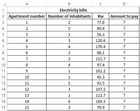
Example 1. When calculating the cost of the amount of consumed kW of electricity for subscribers, the following conditions are taken into account:
- If less than 3 people live in the apartment or less than 100 kW of electricity was consumed per month, the rate per 1 kW is 4.35$.
- In other cases, the rate for 1 kW is 5.25$.
Calculate the amount payable per month for several subscribers.
View source data table:
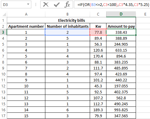
Perform the calculation according to the formula:
Argument Description:
- OR (B3<=2,C3<100) is a logical expression that verifies two conditions: do less than 3 people live in the apartment or does the total amount of energy consumed less than 100 kW? The result of the test will be TRUE if either of these two conditions is true;
- C3 * 4.35 — the amount to be paid, if the OR function returns TRUE;
- C3 * 5.25 is the amount to be paid if OR returns FALSE.
We stretch the formula for the remaining cells using the autocomplete function. The result of the calculation for each subscriber:
Using the AND function in the formula in the first argument in the IF function, we check the conformity of the values by two conditions at once.
Formula with IF and AVERAGE functions for selecting of values by conditions
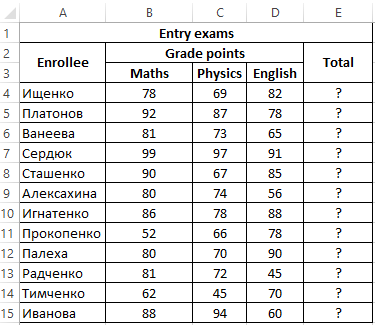
Example 2. Applicants entering the university for the specialty «mechanical engineer» are required to pass 3 exams in mathematics, physics and English. The maximum score for each exam is 100. The average passing score for 3 exams is 75, while the minimum score in physics must be at least 70 points, and in mathematics it is 80. Determine applicants who have successfully passed the exams.
View source table:
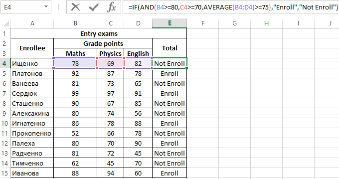
To determine the enrolled students use the formula:
Argument Description:
- AND(B4>=80,C4>=70,AVERAGE(B4:D4)>=75) — checked logical expressions according to the condition of the problem;
- «Enroll» — the result, if the function AND returned the value TRUE (all expressions represented as its arguments, as a result of the calculations returned the value TRUE);
- «Not Enroll» — the result if AND returned FALSE.
Using the autocomplete function (double-click on the cursor marker in the lower right corner), we get the rest of the results:
Formula with logical functions AND IF OR in excel
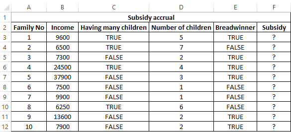
Example 3. Subsidies in the amount of 30% are charged to families with an average income below 8,000$, which are large or there is no main breadwinner. If the number of children is over 5, the amount of the subsidy is 50%. Determine who should receive subsidies and who should not.
View source table:
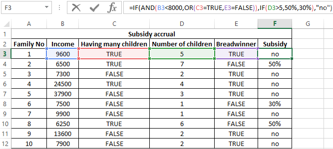
To check the criteria according to the condition of the problem, we write the formula:
Argument Description:
- AND(B3<8000,OR(C3=TRUE,E3=FALSE)) is the checked expression according to the condition of the problem. In this case, the AND function returns the TRUE value, if B3 <8000 is true and at least one of the expressions passed as arguments to the OR function also returns the TRUE value.
- The nested IF function performs a check on the number of children in the family, which rely on subsidies.
- If the main condition returned the result is FALSE, the main function IF returns the text string “no”.
Perform the calculation for the first family and stretch the formula to the remaining cells using the autocomplete function. Results:
Features of using logical functions IF, AND, OR in Excel
The IF function has the following syntax notation:
=IF(Logical_test,[ Value_if_True ],[ Value_if_False])
As you can see, by default, you can check only one condition, for example, is e3 more than 20? Using the IF function, this check can be done as follows:
=IF(EXP(3)>20,»more»,»less»)
As a result, the text string “more” will be returned. If we need to find out if any value belongs to the specified interval, we will need to compare this value with the upper and lower limits of the intervals, respectively. For example, is the result of calculating e3 in the range from 20 to 25? When using the IF function alone, you must enter the following entry:
=IF(EXP(3)>20,IF(EXP(3)<25,»belongs»,»does not belong»),»does not belong»)
We have a nested function IF as one of the possible results of the implementation of the main function IF, and therefore the syntax looks somewhat cumbersome. If you also need to know, for example, whether the square root e3 is equal to a numeric value from a fractional number range from 4 to 5, the final formula will look cumbersome and unreadable.
It is much easier to use as a condition a complex expression that can be written using AND and OR functions. For example, the above function can be rewritten as follows:
=IF(AND(EXP(3)>20,EXP(3)<25),»belongs»,»does not belong»)
The result of the execution of the AND expression (EXP(3)>20,EXP(3)<25) can be a logical value TRUE only if the result of checking each of the specified conditions is a logical value TRUE. In other words, the function AND allows you to test one, two or more hypotheses on their truth, and returns the result FALSE if at least one of them is incorrect.
Sometimes you want to know if at least one assumption is true. In this case, it is convenient to use the OR function, which performs the check of one or several logical expressions and returns a logical TRUE, if the result of the calculations of at least one of them is a logical TRUE. For example, you want to know if e3 is an integer or a number that is less than 100? To test this condition, you can use the following formula:
=IF(OR(MOD(EXP(3),1)<>0,EXP(3)<100),»true»,»false»)
The “<>” means inequality, that is, more or less than some value. In this case, both expressions return the value TRUE, and the result of the execution of the IF function is the text string «true.» However, if an OR test was performed (MOD(EXP (3),1)<>0,EXP(3)<20, while EXP(3) <20 will return FALSE, the result of the calculation of the IF function will not change, since MOD(EXP(3),1) <> 0 returns TRUE.
Download examples using the functions OR AND IF in Excel
In practice, often used bundles IF + AND, IF + OR, or all three functions at once. Consider examples of similar use of these functions.
Things will not always be the way we want them to be. The unexpected can happen. For example, let’s say you have to divide numbers. Trying to divide any number by zero (0) gives an error. Logical functions come in handy such cases. In this tutorial, we are going to cover the following topics.
In this tutorial, we are going to cover the following topics.
- What is a Logical Function?
- IF function example
- Excel Logic functions explained
- Nested IF functions
What is a Logical Function?
It is a feature that allows us to introduce decision-making when executing formulas and functions. Functions are used to;
- Check if a condition is true or false
- Combine multiple conditions together
What is a condition and why does it matter?
A condition is an expression that either evaluates to true or false. The expression could be a function that determines if the value entered in a cell is of numeric or text data type, if a value is greater than, equal to or less than a specified value, etc.
IF Function example
We will work with the home supplies budget from this tutorial. We will use the IF function to determine if an item is expensive or not. We will assume that items with a value greater than 6,000 are expensive. Those that are less than 6,000 are less expensive. The following image shows us the dataset that we will work with.
- Put the cursor focus in cell F4
- Enter the following formula that uses the IF function
=IF(E4<6000,”Yes”,”No”)
HERE,
- “=IF(…)” calls the IF functions
- “E4<6000” is the condition that the IF function evaluates. It checks the value of cell address E4 (subtotal) is less than 6,000
- “Yes” this is the value that the function will display if the value of E4 is less than 6,000
-
“No” this is the value that the function will display if the value of E4 is greater than 6,000
When you are done press the enter key
You will get the following results
Excel Logic functions explained
The following table shows all of the logical functions in Excel
| S/N | FUNCTION | CATEGORY | DESCRIPTION | USAGE |
|---|---|---|---|---|
| 01 | AND | Logical | Checks multiple conditions and returns true if they all the conditions evaluate to true. | =AND(1 > 0,ISNUMBER(1)) The above function returns TRUE because both Condition is True. |
| 02 | FALSE | Logical | Returns the logical value FALSE. It is used to compare the results of a condition or function that either returns true or false | FALSE() |
| 03 | IF | Logical |
Verifies whether a condition is met or not. If the condition is met, it returns true. If the condition is not met, it returns false. =IF(logical_test,[value_if_true],[value_if_false]) |
=IF(ISNUMBER(22),”Yes”, “No”) 22 is Number so that it return Yes. |
| 04 | IFERROR | Logical | Returns the expression value if no error occurs. If an error occurs, it returns the error value | =IFERROR(5/0,”Divide by zero error”) |
| 05 | IFNA | Logical | Returns value if #N/A error does not occur. If #N/A error occurs, it returns NA value. #N/A error means a value if not available to a formula or function. |
=IFNA(D6*E6,0) N.B the above formula returns zero if both or either D6 or E6 is/are empty |
| 06 | NOT | Logical | Returns true if the condition is false and returns false if condition is true |
=NOT(ISTEXT(0)) N.B. the above function returns true. This is because ISTEXT(0) returns false and NOT function converts false to TRUE |
| 07 | OR | Logical | Used when evaluating multiple conditions. Returns true if any or all of the conditions are true. Returns false if all of the conditions are false |
=OR(D8=”admin”,E8=”cashier”) N.B. the above function returns true if either or both D8 and E8 admin or cashier |
| 08 | TRUE | Logical | Returns the logical value TRUE. It is used to compare the results of a condition or function that either returns true or false | TRUE() |
A nested IF function is an IF function within another IF function. Nested if statements come in handy when we have to work with more than two conditions. Let’s say we want to develop a simple program that checks the day of the week. If the day is Saturday we want to display “party well”, if it’s Sunday we want to display “time to rest”, and if it’s any day from Monday to Friday we want to display, remember to complete your to do list.
A nested if function can help us to implement the above example. The following flowchart shows how the nested IF function will be implemented.
The formula for the above flowchart is as follows
=IF(B1=”Sunday”,”time to rest”,IF(B1=”Saturday”,”party well”,”to do list”))
HERE,
- “=IF(….)” is the main if function
- “=IF(…,IF(….))” the second IF function is the nested one. It provides further evaluation if the main IF function returned false.
Practical example
Create a new workbook and enter the data as shown below
- Enter the following formula
=IF(B1=”Sunday”,”time to rest”,IF(B1=”Saturday”,”party well”,”to do list”))
- Enter Saturday in cell address B1
- You will get the following results
Download the Excel file used in Tutorial
Summary
Logical functions are used to introduce decision-making when evaluating formulas and functions in Excel.
A logical test means having an analytical output that is either TRUE or FALSE. In Excel, we can perform a logical test for any situation. The most commonly used logical test is using the equals to the operator, which is “=” if we use =A1=B1 in cell A2, then it will return TRUE if the values are equal and FALSE if the values are not equal.
What is the Logical Test in Excel?
In Excel, at the beginning stages of learning, it is not easy to understand the concept of logical tests. But once you master this, it will be a valuable skill for your CV. More often than not, in Excel, we use a logical test to match multiple criteriaCriteria based calculations in excel are performed by logical functions. To match single criteria, we can use IF logical condition, having to perform multiple tests, we can use nested IF conditions. But for matching multiple criteria to arrive at a single result is a complex criterion-based calculation.read more and arrive at the desired solution.
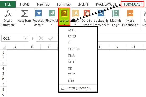
In Excel, we have as many as 9 logical formulas. We must go to the “Formulas” tab and click on the “Logical” function group to see the logical formulas.
Some of them are frequently used formulas, and some of them are rarely used. This article will cover some of the important Excel logical formulas in real-time examples. All the Excel logical formulas work based on TRUE or FALSE if the logical test we do.
Table of contents
- What is the Logical Test in Excel?
- How to Use Logical Function in Excel?
- #1 – AND & OR Logical Function in Excel
- Example #1- AND Logical Function in Excel
- Example #2 – OR Logical Function in Excel
- #2 – IF Logical Function in Excel
- #3 – IF with AND & OR Logical Functions in Excel
- Things to Remember
- Recommended Articles
How to Use Logical Function in Excel?
Below are examples of logical functions in Excel.
You can download this Logical Functions Excel Template here – Logical Functions Excel Template
#1 – AND & OR Logical Function in Excel
Excel AND and OR functions work opposite each other. For example, AND condition in Excel requires all the logical tests to be TRUE. On the other hand, the OR function requires any logical tests to be TRUE.
For example, look at the below examples.
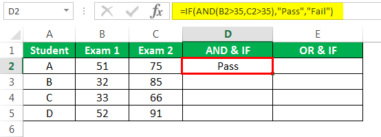
We have student names, marks 1, and marks 2. If the student scored more than 35 in both exams, the result should be TRUE. If not, the result should be FALSE. Since we need to satisfy both the conditions, we need to use AND logical test here.
Example #1- AND Logical Function in Excel
- We must open AND function first.
- The first logical 1 is Marks-1 is >35 or not to test the condition.
- The second test is Marks-2 is >35 or not. So, we must take the logical test.
- We have only two conditions to test. So, we have applied both the logical tests. Now close the bracket.
If both conditions are satisfied, the formula returns TRUE by default. Else, returns FALSE as a result.
Drag the formula to the rest of the cells.
In cells D3 and D4, we got FALSE because in “Marks-1,” both the students scored less than 35.
Example #2 – OR Logical Function in Excel
The Excel OR function is completely different from the AND function. The OR in ExcelThe OR function in Excel is used to test various conditions, allowing you to compare two values or statements in Excel. If at least one of the arguments or conditions evaluates to TRUE, it will return TRUE. Similarly, if all of the arguments or conditions are FALSE, it will return FASLE.read more requires only one condition to be TRUE. Therefore, we must apply the same logical test to the above data with OR conditions.
We will have results in either FALSE or TRUE. Here, we got TRUE.
Drag the formula to other cells.
Now, look at the difference between AND and OR functions. The OR function returns TRUE for students B and C even though they have scored less than 35 in one of the exams. However, since they scored more than 35 in Marks 2, the OR function found the condition of >35 TRUE in 2 logical tests and returned TRUE as a result.
#2 – IF Logical Function in Excel
The IF excel FunctionIF function in Excel evaluates whether a given condition is met and returns a value depending on whether the result is “true” or “false”. It is a conditional function of Excel, which returns the result based on the fulfillment or non-fulfillment of the given criteria.
read more is one of the important logical functions to discuss in Excel. It includes three arguments to supply. Now, look at the syntax.
- Logical Test: It is nothing but our conditional test.
- Value if True: If the above logical test in Excel is TRUE, what should be the result.
- Values if FALSE: If the above logical test in Excel is FALSE, what should be the result.
For example, take a look at the below data.
If the product’s price is more than 80, we need the result as “Costly.” On the other hand, if the product’s price is less than 80, we need the result as “OK.”
Step 1: Here, the logical test is whether the price is >80 or not. So, we must open the IF condition first.
Step 2: Now pass the logical test in Excel, Price >80.
Step 3: If the logical test in Excel is TRUE, we need the result as “Costly.” So in the next argument, VALUE, if TRUE, mentions the result in double-quotes as “Costly.”
Step 4: The final argument is if the logical test in Excel is FALSE. If the test is FALSE, we need the result to be “OK.”
We got the result of “Costly.”
Step 5: Drag the formula to other cells to have the result in all the cells.
Since the orange and sapota price is less than 80, we got the result as “OK.” However, the logical test in Excel is >80, so we got “Costly” for apples and grapes because their price is > 80.
#3 – IF with AND & OR Logical Functions in Excel
The IF function with the other two logical functions (AND & OR) is one of the best combination formulas in Excel. For better understanding, look at the below example data, which we have used for AND and OR conditions.
If the student scored more than 35 in both the exams, it would declare him a PASS or FAIL.
The AND function, by default, can only return TRUE or FALSE as a result. But here, we need the results as PASS or FAIL. So, we have to use the IF condition here.
Open the IF condition first.
If we can only test one condition simultaneously, we need to look at two conditions. So, we must open AND condition and pass the tests as Exam 1 >35 and Exam 2>35.
If both the supplied conditions are TRUE, we need the result as “PASS.” So mention the value “PASS” if the logical test in Excel is “TRUE.”
If the logical test in Excel is “FALSE,” the result should be “FAIL.”
So, here we got the result as “PASS.”
Drag the formula to other cells.
So, instead of default TRUE or FALSE, we got our values with the help of the IF condition. Similarly, we can also apply the OR function and replace the OR function with the IF and AND functions.
Things to Remember
- The AND functionThe AND function in Excel is classified as a logical function; it returns TRUE if the specified conditions are met, otherwise it returns FALSE.read more requires all the logical tests in Excel to be TRUE.
- The OR function requires at least any logical tests to be TRUE.
- We have other logical tests in Excel like the IFERROR function in excelThe IFERROR function in Excel checks a formula (or a cell) for errors and returns a specified value in place of the error.read more, NOT function in excelNOT Excel function is a logical function in Excel that is also known as a negation function and it negates the value returned by a function or the value returned by another logical function.read more, TRUE Function in excelIn Excel, the TRUE function is a logical function that is used by other conditional functions such as the IF function. If the condition is met, the output is true; if the conditions are not met, the output is false.read more, FALSE, etc.…
- We will discuss the remaining Excel logical tests in a separate article.
Recommended Articles
This article is a guide to Logical Tests in Excel. We discuss logical functions like AND, OR, and IF in Excel, practical examples, and a downloadable template. You may also learn more about Excel from the following articles: –
- SUMIF with Multiple CriteriaThe SUMIF (SUM+IF) with multiple criteria sums the cell values based on the conditions provided. The criteria are based on dates, numbers, and text. The SUMIF function works with a single criterion, while the SUMIFS function works with multiple criteria in excel.read more
- IFERROR in Excel VBAThe IFERROR function in Excel is used to determine what to do when an error occurs before performing any function.read more
- SUMPRODUCT in Excel with Multiple CriteriaIn Excel, using SUMPRODUCT with several Criteria allows you to compare different arrays using multiple criteria.read more
- VLookup Function with IFIn Excel, vlookup is a reference function, and IF is a conditional statement. Based on the results of the Vlookup function, they locate a value that meets the criteria and also matches the reference value.read more
To write an IF, AND, OR array formula in Excel 365, we must use the arithmetic operators * (multiplication) and + (addition). Why it’s so?
If we take the logical AND, OR with the IF in Excel 365 to spill the result, we won’t get our expected result.
I mean, such a formula won’t support a range/array in evaluation. Even if it supports, it won’t return an array result.
So we will replace the AND logical operator with the * (multiplication) and OR with the + (addition) arithmetic operators.
Coding the formula with the said two operators is very simple and easily readable.
I think I can convince you the same with the examples below.
Example to IF, AND, OR in Excel 365 (Non-Array Formula)
Imagine a user played a game three times, and we have recorded his scores out of 100 in cells A2, B2, and C2.
We want to perform the following three logical tests on the scores individually.
- If all scores are >=80, return OK.
- If any of the two scores are >=80, return OK.
- Finally, if any of the scores is >=80, return OK.
Logical Tests Using IF, AND, OR Functions
In Excel, we can perform the above three logical tests as follows.
1. E2 (If all scores are >=80, return OK)
=IF(AND(A2>=80,B2>=80,C2>=80),"OK","NOT OK")I have used the AND function with IF in the above Excel formula to test if all the three logical tests return TRUE.
2. F2 (If any of the two scores are >=80, return OK)
We must use the following logic (two parts) to test if any two logical tests return TRUE.
AND Part:-
a) Value 1>=80 and value 2>=80.
b) Value 1>=80 and value 3>=80.
c) Value 2>=80 and value 3>=80.
OR Part:-
a) The OR evaluates to TRUE if any two of the above three AND tests return TRUE.
So the formula will be as follows.
=IF(OR(AND(A2>=80,B2>=80),AND(A2>=80,C2>=80),AND(B2>=80,C2>=80)),"OK","NOT OK")It is an example of the IF, AND, OR logical test in Excel.
3. G2 (if any of the scores is >=80, return OK)
=IF(OR(A2>=80,B2>=80,C2>=80),"OK","NOT OK")Here I have used the OR function with IF to test if any of the three logical tests return TRUE.
As I have already mentioned, we can’t write an IF, AND, OR array formula as above in Excel 365.
Logical Tests Using IF, *, + Formula
Let’s substitute the above three formulas by replacing AND, OR with multiplication and addition.
But that’s not enough. Then?
The below formulas are self-explanatory.
1. E2 Formula
=IF((A2:A8>=80)*(B2:B8>=80)*(C2:C8>=80),"OK","NOT OK")How the multiplication replaces the logical function OR above?
Each test in the formula returns either TRUE or FALSE. If all the criteria are met, it will be =IF((TRUE*TRUE*TRUE),"OK","NOT OK").
We can even replace the multiplication operator here with addition.
=IF((A2:A8>=80)+(B2:B8>=80)+(C2:C8>=80)>2,"OK","NOT OK")Please remember that the value of TRUE is 1, and FALSE is 0.
2. F2 Formula
=IF((A2:A8>=80)+(B2:B8>=80)+(C2:C8>=80)>1,"OK","NOT OK")3. G2 Formula
=IF((A2:A8>=80)+(B2:B8>=80)+(C2:C8>=80)>0,"OK","NOT OK")Above I have tried to simplify the use of the logical operators within the IF function.
Now let’s open an Excel Spreadsheet and enter the scores of multiple players in the range A2:C8 as below.
So the values to evaluate are in cell range A2:C8.
I have inserted the following three IF, AND, OR array formulas in cells E2, F2, and G2, respectively.
1. E2 Array Formula
=IF((A2:A8>=80)*(B2:B8>=80)*(C2:C8>=80),"OK","NOT OK")2. F2 Array Formula
=IF((A2:A8>=80)+(B2:B8>=80)+(C2:C8>=80)>1,"OK","NOT OK")3. G2 Array Formula
=IF((A2:A8>=80)+(B2:B8>=80)+(C2:C8>=80)>0,"OK","NOT OK")If any of the above formulas return #SPILL!, please empty the cells down in that column.
Nested IF, AND, OR Combination in Excel 365
I want to assign grades based on the scores above.
In that case, we may require to write a nested IF, AND, OR combination array formula in Excel 365.
Here is how.
In the above example, we have used three formulas for the below three logical tests.
- If all scores are >=80, return OK.
- If any of the two scores are >=80, return OK.
- Finally, if any of the scores is >=80, return OK.
There each test returns OK or NOT OK.
Instead of that, here, I want the tests to return GR-1, GR-2, and GR-3.
- If all scores are >=80, return GR-1.
- If any of the two scores are >=80, return GR-2.
- Finally, if any of the scores is >=80, return GR-3.
For that, we should combine the above three IF, AND, OR Array Formulas.
How?
In the E2 formula, replace “OK” with “GR-1” and “NOT OK” with the F2 formula.
In that combined (E2 and F2) formula, replace “OK” with “GR-2” and “NOT OK” with the G2 formula.
Then, in the combined E2, F2, and G2 formula, replace “OK” with “GR-3” and replace “NOT OK” with “F.”
Here it is.
=IF(
     (A2:A8>=80)*(B2:B8>=80)*(C2:C8>=80),"GR-1",
     IF(
        (A2:A8>=80)+(B2:B8>=80)+(C2:C8>=80)>1,"GR-2",
        IF(
           (A2:A8>=80)+(B2:B8>=80)+(C2:C8>=80)>0,"GR-3","F"
        )
     )
)
We can call it a nested IF, AND, OR combination array formula.
Related:- How to Use the IFS Function in Excel 365.


