
Excel for Microsoft 365 Excel for Microsoft 365 for Mac Excel 2021 Excel 2021 for Mac Excel 2019 Excel 2019 for Mac Excel 2016 Excel 2016 for Mac Excel 2013 Excel 2010 Excel 2007 More…Less
IF is one of the most versatile and popular functions in Excel, and is often used multiple times in a single formula, as well as in combination with other functions. Unfortunately, because of the complexity with which IF statements can be built, it is fairly easy to run into the #VALUE! error. You can usually suppress the error by adding error-handling specific functions like ISERROR, ISERR, or IFERROR to your formula.
Problem: The argument refers to error values
When there is a cell reference to an error value, IF displays the #VALUE! error.
Solution: You can use any of the error-handling formulas such as ISERROR, ISERR, or IFERROR along with IF. The following topics explain how to use IF, ISERROR and ISERR, or IFERROR in a formula when your argument refers to error values.
-
Correct the #VALUE! error in the CONCATENATE function
-
Correct the #VALUE! error in AVERAGE or SUM functions
Notes:
-
IFERROR was introduced in Excel 2007, and is far more preferable to ISERROR or ISERR, as it doesn’t require a formula to be constructed redundantly. ISERROR and ISERR force a formula to be calculated twice, first to see if it evaluates to an error, then again to return its result. IFERROR only calculates once.
-
=IFERROR(Formula,0) is much better than =IF(ISERROR(Formula,0,Formula))
Problem: The syntax is incorrect
If a function’s syntax is not constructed correctly, it can return the #VALUE! error.
Solution: Make sure you are constructing the syntax properly. Here’s an example of a well-constructed formula that nests an IF function inside another IF function to calculate deductions based on income level.
=IF(E2<31500,E2*15%,IF(E2<72500,E2*25%,E2*28%))

In simple English this means — IF(the value in cell A5 is less than 31,500, then multiply the value by 15%. But IF it’s not, check to see if the value is less than 72,500. IF it is, multiply by 25%, otherwise multiply by 28%).
To use IFERROR with an existing formula, you just wrap the completed formula with IFERROR:
=IFERROR(IF(E2<31500,E2*15%,IF(E2<72500,E2*25%,E2*28%)),0)
Which simply says IF any part of the original formula evaluates to an error, then display 0, otherwise return the result of the IF statement. Some people write their formulas complete with error handling to start, however this isn’t good practice, since the error handler will suppress any potential errors, so you won’t necessarily know if your formula is working properly or not. If you need to add error handling, it’s best to add it once you’re sure your formula works properly.
Note: The evaluation values in formulas don’t have commas. If you add them, the IF function will try to use them as arguments and Excel will yell at you. On the other hand, the percentage multipliers have the % symbol. This tells Excel you want those values to be seen as percentages. Otherwise, you would need to enter them as their actual percentage values, like “E2*0.25”.

Need more help?
You can always ask an expert in the Excel Tech Community or get support in the Answers community.
See Also
Correct a #VALUE! error
IF function
IFERROR function
IS functions
IFS function (Microsoft 365 or Excel 2016 or later)
IF function – nested formulas and avoiding pitfalls
Video: Nested IF functions
Overview of formulas in Excel
How to avoid broken formulas
Detect errors in formulas
All Excel functions (alphabetical)
All Excel functions (by category)
Need more help?
 In this Excel IFERROR, ISERROR, ISERR, IFNA and ISNA Tutorial, you learn how to use the IFERROR, ISERROR, ISERR, IFNA and ISNA functions in your worksheet formulas for the following:
- Identify errors, including the #N/A error.
- Handle errors, including the #N/A error, and return a specific:
- Value;
- Formula;
- Expression; or
- Reference.
- Carry out VLookups that handle errors, including the #N/A error, and return a specific:
- Value;
- Formula;
- Expression; or
- Reference.
- Check whether a specific value exists in a list or compare 2 columns.
This Excel IFERROR, ISERROR, ISERR, IFNA and ISNA Tutorial is accompanied by an Excel workbook containing the data and formulas I use in the examples below. You can get immediate free access to this example workbook by subscribing to the Power Spreadsheets Newsletter.
Use the following Table of Contents to navigate to the section you’re interested in.
Related Excel Tutorials
The following Tutorials may help you better understand and implement the contents below:
- Formulas and functions:
- Learn how to work with the LEFT, RIGHT, MID, LEN, FIND and SEARCH functions here.
- Macros and VBA:
- Learn how to use worksheet functions in macros here.
- Learn how to work with the VLookup function in VBA here.
You can find additional Tutorials in the Archives.
IFERROR formula
To handle possible errors with the IFERROR function, use a formula with the following structure:
=IFERROR(Value,ValueIfError)
IFERROR process
To handle possible errors with the IFERROR function, follow these steps:
- Specify the expression you want to check for errors (Value).
- Specify that, if Value returns an error (IFERROR), another value (ValueIfError) is returned.
IFERROR formula explanation
Item: IFERROR
The IFERROR function:
- Returns the value you specify (ValueIfError) if an expression (Value) returns an error; and
- Returns the result of that expression (Value) otherwise.
In other words, IFERROR does the following:
- Checks an expression (Value).
- If Value returns an error, IFERROR returns the value you specify (ValueIfError).
- If Value doesn’t return an error, IFERROR returns the result of that expression.
Therefore, you usually use IFERROR to trap and handle errors in worksheet formulas. The IFERROR function deals with the following errors:
- #N/A.
- #VALUE!
- #REF!
- #DIV/0!
- #NUM!
- #NAME?
- #NULL!
Item: Value
The value argument of the IFERROR function (Value) is a value, formula, expression or reference that Excel checks for errors.
If Value doesn’t return an error, IFERROR returns the result of that expression.
Item: ValueIfError
The value_if_error argument of the IFERROR function (ValueIfError) is the value, formula, expression or reference that Excel returns if the value argument of the IFERROR function (Value) evaluates to an error.
IFERROR formula example
The worksheet formulas below handle possible errors with the IFERROR function, as follows:
- Value: The quotient obtained by dividing:
- The value specified in column G (G12 to G16); by
- The value specified in column F (F12 to F16).
- ValueIfError: The string “Total Sales are $ 0” (“Total Sales are $ 0”).
| No. | IFERROR formula |
| 1 | =IFERROR(G12/F12,"Total Sales are $ 0") |
| 2 | =IFERROR(G13/F13,"Total Sales are $ 0") |
| 3 | =IFERROR(G14/F14,"Total Sales are $ 0") |
| 4 | =IFERROR(G15/F15,"Total Sales are $ 0") |
| 5 | =IFERROR(G16/F16,"Total Sales are $ 0") |
Effects of using IFERROR formula example
The following image illustrates the results returned by the IFERROR formula that handles possible errors. As expected, the formulas (in cells H12 to H16):
- Check an expression (Value) for errors; and
- Return the following:
- If Value returns an error: The string “Total Sales are $ 0” (ValueIfError).
- If Value doesn’t return an error: Value itself.
Notice the difference between the result returned by the IFERROR formula that handles errors in cell H16 and the result returned by the regular formula (without IFERROR) in cell H11.

#2: IFERROR then 0
IFERROR then 0 formula
To return 0 if an expression returns an error (with the IFERROR function), use a formula with the following structure:
IFERROR then 0 process
To return 0 if an expression returns an error (with the IFERROR function), follow these steps:
- Specify the expression you want to check for errors (Value).
- Specify that, if Value returns an error (IFERROR), 0 (0) is returned.
IFERROR then 0 formula explanation
Item: IFERROR
The IFERROR function:
- Returns the value you specify (0) if an expression (Value) returns an error; and
- Returns the result of that expression (Value) otherwise.
In other words, IFERROR does the following:
- Checks an expression (Value).
- If Value returns an error, IFERROR returns the value you specify (0).
- If Value doesn’t return an error, IFERROR returns the result of that expression.
Therefore, you usually use IFERROR to trap and handle errors in worksheet formulas. The IFERROR function deals with the following errors:
- #N/A.
- #VALUE!
- #REF!
- #DIV/0!
- #NUM!
- #NAME?
- #NULL!
Item: Value
The value argument of the IFERROR function (Value) is a value, formula, expression or reference that Excel checks for errors.
If Value doesn’t return an error, IFERROR returns the result of that expression.
Item: 0
The value_if_error argument of the IFERROR function (0) is the value, formula, expression or reference that Excel returns if the value argument of the IFERROR function (Value) evaluates to an error.
To return 0 if an expression (Value) returns an error, set value_if_error to 0.
IFERROR then 0 formula example
The worksheet formulas below return 0 if an expression returns an error (with the IFERROR function), where Value is the quotient obtained by dividing:
- The value specified in column G (G22 to G26); by
- The value specified in column F (F22 to F26).
| No. | IFERROR then 0 formula |
| 1 | =IFERROR(G22/F22,0) |
| 2 | =IFERROR(G23/F23,0) |
| 3 | =IFERROR(G24/F24,0) |
| 4 | =IFERROR(G25/F25,0) |
| 5 | =IFERROR(G26/F26,0) |
Effects of using IFERROR then 0 formula example
The following image illustrates the results returned by the IFERROR formula that handles possible errors by returning 0. As expected, the formulas (in cells H22 to H26):
- Check an expression (Value) for errors; and
- Return the following:
- If Value returns an error: 0.
- If Value doesn’t return an error: Value itself.
Notice the difference between the result returned by the IFERROR formula that handles errors by returning 0 in cell H26 and the result returned by the regular formula (without IFERROR then 0) in cell H21.

#3: IFERROR then blank
IFERROR then blank formula
To return a blank if an expression returns an error (with the IFERROR function), use a formula with the following structure:
IFERROR then blank process
To return a blank if an expression returns an error (with the IFERROR function), follow these steps:
- Specify the expression you want to check for errors (Value).
- Specify that, if Value returns an error (IFERROR), a zero-length string (“”) is returned.
IFERROR then blank formula explanation
Item: IFERROR
The IFERROR function:
- Returns the value you specify (“”) if an expression (Value) returns an error; and
- Returns the result of that expression (Value) otherwise.
In other words, IFERROR does the following:
- Checks an expression (Value).
- If Value returns an error, IFERROR returns the value you specify (“”).
- If Value doesn’t return an error, IFERROR returns the result of that expression.
Therefore, you usually use IFERROR to trap and handle errors in worksheet formulas. The IFERROR function deals with the following errors:
- #N/A.
- #VALUE!
- #REF!
- #DIV/0!
- #NUM!
- #NAME?
- #NULL!
Item: Value
The value argument of the IFERROR function (Value) is a value, formula, expression or reference that Excel checks for errors.
If Value doesn’t return an error, IFERROR returns the result of that expression.
Item: “”
The value_if_error argument of the IFERROR function (“”) is the value, formula, expression or reference that Excel returns if the value argument of the IFERROR function (Value) evaluates to an error.
To return a blank if an expression (Value) returns an error, set value_if_error to a zero-length string (“”).
IFERROR then blank formula example
The worksheet formulas below return a blank if an expression returns an error (with the IFERROR function), where Value is the quotient obtained by dividing:
- The value specified in column G (G32 to G36); by
- The value specified in column F (F32 to F36).
| No. | IFERROR then blank formula |
| 1 | =IFERROR(G32/F32,"") |
| 2 | =IFERROR(G33/F33,"") |
| 3 | =IFERROR(G34/F34,"") |
| 4 | =IFERROR(G35/F35,"") |
| 5 | =IFERROR(G36/F36,"") |
Effects of using IFERROR then blank formula example
The following image illustrates the results returned by the IFERROR formula that handles possible errors by returning a blank (“”). As expected, the formulas (in cells H32 to H36):
- Check an expression (Value) for errors; and
- Return the following:
- If Value returns an error: A zero-length string (“”).
- If Value doesn’t return an error: Value itself.
Notice the difference between the result returned by the IFERROR formula that handles errors by returning a blank in cell H36 and the result returned by the regular formula (without IFERROR then blank) in cell H31.

#4: IFERROR VLOOKUP
IFERROR VLOOKUP formula
To carry out a VLookup that handles possible errors (with IFERROR vs. IFNA), use a formula with the following structure:
=IFERROR(VLOOKUP(LookupValue,LookupTable,ColumnIndex,RangeLookup),ValueIfError)
IFERROR VLOOKUP process
To carry out a VLookup that handles possible errors (with IFERROR vs. IFNA), follow these steps:
- Specify the value you want to look up (LookupValue) in the first (leftmost) column of a table (LookupTable).
- Identify the cell range (a table array) containing the lookup table (LookupTable).
- Specify the index number of the column (within LookupTable) from which you want to obtain a value (ColumnIndex).
- Specify whether VLOOKUP searches for an exact or approximate match (RangeLookup).
- Specify that, if VLOOKUP returns an error (IFERROR), another value (ValueIfError) is returned.
IFERROR VLOOKUP formula explanation
Formula #1: VLOOKUP(LookupValue,LookupTable,ColumnIndex,RangeLookup)
Item: VLOOKUP
The VLOOKUP function does the following:
- Looks for a value (LookupValue) in the first (leftmost) column of a table (LookupTable); and
- Returns a value in the same row but from another column you specify (ColumnIndex).
Item: LookupValue
The lookup_value argument of the VLOOKUP function (LookupValue) is the value you look up in the first (leftmost) column of LookupTable. In other words, LookupValue must usually be in the first column of the cell range you specify as LookupTable.
If VLOOKUP doesn’t find LookupValue in the first column of LookupTable, it usually returns the #N/A error.
You can specify LookupValue as either:
- A value;
- A text string; or
- A cell reference.
Item: LookupTable
The table_array argument of the VLOOKUP function (LookupTable) is the cell range in which VLOOKUP searches for the following:
- The LookupValue in the first column of LookupTable; and
- The value to return in the column you specify (ColumnIndex).
Therefore, the cell range you specify as LookupTable must usually include both of the following columns:
- The first column, which must contain the LookupValue; and
- The column from which VLOOKUP should return a value.
If VLOOKUP doesn’t find LookupValue in the first column of LookupTable, it usually returns the #N/A error.
Item: ColumnIndex
The col_index_num argument of the VLOOKUP function (ColumnIndex) is the column number within the LookupTable from which VLOOKUP returns a value, as follows:
| Column | ColumnIndex | Comments |
| First | 1 | Must usually contain the LookupValue. Otherwise, VLOOKUP usually returns the #N/A error. |
| Second | 2 | |
| Third | 3 | |
| … | … | |
| #th | # |
Item: RangeLookup
The range_lookup argument of the VLOOKUP function (RangeLookup) specifies whether VLOOKUP searches for an approximate or an exact match for LookupValue in the first column of LookupTable.
- Set RangeLookup to TRUE when searching for an approximate match.
- Set RangeLookup to FALSE when searching for an exact match.
Formula #2: IFERROR(VLOOKUP(…),ValueIfError)
Item: IFERROR
The IFERROR function:
- Returns the value you specify (ValueIfError) if an expression (VLOOKUP(…)) returns an error; and
- Returns the result of that expression (VLOOKUP(…)) otherwise.
In other words, IFERROR does the following:
- Checks an expression (VLOOKUP(…)).
- If VLOOKUP(…) returns an error, IFERROR returns the value you specify (ValueIfError).
- If VLOOKUP(…) doesn’t return an error, IFERROR returns the result of that formula.
Item: VLOOKUP(…)
The value argument of the IFERROR function (VLOOKUP(…)) is a value, formula, expression or reference that Excel checks for errors.
If VLOOKUP(….) doesn’t return an error, IFERROR returns the result of that formula. For the explanation of this VLOOKUP function, please refer to the appropriate section in this Tutorial.
One of the most common errors returned by the VLOOKUP function is #N/A. The VLOOKUP function usually returns an #N/A error when you either:
- Give an inappropriate value (including a value that isn’t found in the first column of LookupTable) for the lookup_value argument (LookupValue); or
- Use the function to locate a value in a table (LookupTable) that isn’t properly sorted.
Item: ValueIfError
The value_if_error argument of the IFERROR function (ValueIfError) is the value, formula, expression or reference that Excel returns if the value argument of the IFERROR function (VLOOKUP(…)) evaluates to an error.
IFERROR VLOOKUP formula example
The worksheet formula below carries out an exact match VLookup and handles possible errors (with IFERROR vs. IFNA), as follows:
- LookupValue: The value specified in cell M8 ($M$8).
- LookupTable: The lookup table in cells A8 to E57 ($A$8:$E$57).
- ColumnIndex: The column number specified in column K (K10).
- RangeLookup: FALSE.
- ValueIfError: The string “Sales Manager not found” (“Sales Manager not found”).
=IFERROR(VLOOKUP($M$8,$A$8:$E$57,K10,FALSE),"Sales Manager not found")
Effects of using IFERROR VLOOKUP formula example
The following images illustrate the results returned by the IFERROR VLOOKUP formula that carries out a VLookup that handles possible errors (with IFERROR vs. IFNA).
The image below displays the LookupTable.

The image below displays the results returned by IFERROR VLOOKUP. As expected, the formula in cell M10 does the following:
- Looks for the value (LookupValue) specified in cell M8 (Shawn Brooks) in the first column (column A) of the lookup table (LookupTable).
- The LookupValue (Shawn Brooks) isn’t found in the first column of LookupTable. Therefore, the IFERROR VLOOKUP formula returns “Sales Manager not found”.
Notice the difference between the result returned by the IFERROR VLOOKUP formula that handles errors (cell M10) and the result returned by the regular VLOOKUP formula in cell M9 (#N/A).
")
#5: ISERROR
ISERROR formula
To check whether an expression returns an error (with the ISERROR function), use a formula with the following structure:
ISERROR process
To check whether an expression returns an error (with the ISERROR function), specify the expression you want to check for errors (Value).
ISERROR formula explanation
Item: ISERROR
The ISERROR function:
- Tests whether an expression (Value) returns an error; and
- Returns:
- TRUE if Value returns an error; or
- FALSE otherwise.
The ISERROR function identifies the following errors:
- #N/A.
- #VALUE!
- #REF!
- #DIV/0!
- #NUM!
- #NAME?
- #NULL!
Item: Value
The value argument of the ISERROR function (Value) is a value, formula, expression or reference that Excel checks for errors.
ISERROR formula example
The worksheet formulas below check whether an expression returns an error (with the ISERROR function), where Value is the quotient obtained by dividing:
- The value specified in column G (G42 to G46); by
- The value specified in column F (F42 to F46).
| No. | ISERROR formula |
| 1 | =ISERROR(G42/F42) |
| 2 | =ISERROR(G43/F43) |
| 3 | =ISERROR(G44/F44) |
| 4 | =ISERROR(G45/F45) |
| 5 | =ISERROR(G46/F46) |
Effects of using ISERROR formula example
The following image illustrates the results returned by the ISERROR formula that checks whether an expression returns an error. As expected, the formulas (in cells H42 to H46):
- Check an expression (Value) for errors; and
- Return the following:
- TRUE: If Value returns an error.
- FALSE: If Value doesn’t return an error.
Notice the difference between the result returned by the ISERROR formula that checks whether an expression returns an error in cell H46 and the result returned by the regular formula (without ISERROR) in cell H41.

#6: IF ISERROR
IF ISERROR formula
To handle possible errors (with IF ISERROR vs. IFERROR), use a formula with the following structure:
=IF(ISERROR(Value),ValueIfError,Value)
IF ISERROR process
To handle possible errors (with IF ISERROR vs. IFERROR), follow these steps:
- Specify the expression you want to check for errors (Value).
- Test whether Value returns an error (ISERROR) and specify (IF) that:
- If Value returns an error, another value (ValueIfError) is returned; and
- If Value doesn’t return an error, Value itself is returned.
IF ISERROR formula explanation
Formula #1: ISERROR(Value)
Item: ISERROR
The ISERROR function:
- Tests whether an expression (Value) returns an error; and
- Returns:
- TRUE if Value returns an error; or
- FALSE otherwise.
The ISERROR function identifies the following errors:
- #N/A.
- #VALUE!
- #REF!
- #DIV/0!
- #NUM!
- #NAME?
- #NULL!
Item: Value
The value argument of the ISERROR function (Value) is a value, formula, expression or reference that Excel checks for errors.
If Value doesn’t return an error, IF returns the result of that expression. For the explanation of this IF function, please refer to the appropriate section in this Tutorial.
Formula #2: IF(ISERROR(…),ValueIfError,Value)
Item: IF
The IF function:
- Tests whether a condition (ISERROR(…)) is met; and
- Returns:
- One value (ValueIfError) if the condition (ISERROR(…)) is met and returns TRUE; and
- Another value (Value) if the condition (ISERROR(…)) isn’t met and returns FALSE.
Item: ISERROR(…)
The logical_test argument of the IF function (ISERROR(…)) is the condition Excel tests and evaluates to either:
- TRUE; or
- FALSE.
For the explanation of this ISERROR function, please refer to the appropriate section in this Tutorial.
Item: ValueIfError
The value_if_true argument of the IF function (ValueIfError) is the value, formula, expression or reference that Excel returns if ISERROR(…) returns TRUE.
In other words, ValueIfError is the value, formula, expression or reference that Excel returns if the value argument of the ISERROR function (Value) returns an error.
Item: Value
The value_if_false argument of the IF function (Value) is the value, formula, expression or reference that Excel returns if ISERROR(…) returns FALSE.
In other words, Value is the value, formula, expression or reference that Excel returns if the value argument of the ISERROR function (Value itself) doesn’t return an error.
IF ISERROR formula example
The worksheet formulas below handle possible errors (with IF ISERROR vs. IFERROR), as follows:
- Value: The quotient obtained by dividing:
- The value specified in column G (G52 to G56); by
- The value specified in column F (F52 to F56).
- ValueIfError: The string “Total Sales are $ 0” (“Total Sales are $ 0”).
| No. | IF ISERROR formula |
| 1 | =IF(ISERROR(G52/F52),"Total Sales are $ 0",G52/F52) |
| 2 | =IF(ISERROR(G53/F53),"Total Sales are $ 0",G53/F53) |
| 3 | =IF(ISERROR(G54/F54),"Total Sales are $ 0",G54/F54) |
| 4 | =IF(ISERROR(G55/F55),"Total Sales are $ 0",G55/F55) |
| 5 | =IF(ISERROR(G56/F56),"Total Sales are $ 0",G56/F56) |
Effects of using IF ISERROR formula example
The following image illustrates the results returned by the IF ISERROR formula that handles possible errors (with IF ISERROR vs. IFERROR). As expected, the formulas (in cells H52 to H56):
- Check an expression (Value) for errors; and
- Return the following:
- If Value returns an error: The string “Total Sales are $ 0” (ValueIfError).
- If Value doesn’t return an error: Value itself.
Notice the difference between the result returned by the IF ISERROR formula that handles errors in cell H56 and the result returned by the regular formula (without IF ISERROR) in cell H51.
")
#7: IF ISERROR VLOOKUP
IF ISERROR VLOOKUP formula
To carry out a VLookup that handles possible errors (with IF ISERROR vs. IFERROR), use a formula with the following structure:
=IF(ISERROR(VLOOKUP(LookupValue,LookupTable,ColumnIndex,RangeLookup)),ValueIfError,VLOOKUP(LookupValue,LookupTable,ColumnIndex,RangeLookup))
IF ISERROR VLOOKUP process
To carry out a VLookup that handles possible errors (with IF ISERROR vs. IFERROR), follow these steps:
- Specify the value you want to look up (LookupValue) in the first (leftmost) column of a table (LookupTable).
- Identify the cell range (a table array) containing the lookup table (LookupTable).
- Specify the index number of the column (within LookupTable) from which you want to obtain a value (ColumnIndex).
- Specify whether VLOOKUP searches for an exact or approximate match (RangeLookup).
- Test whether VLOOKUP returns an error (ISERROR) and specify (IF) that:
- If VLOOKUP returns an error, another value (ValueIfError) is returned; and
- If VLOOKUP doesn’t return an error, the result of VLOOKUP is returned.
IF ISERROR VLOOKUP formula explanation
Formula #1: VLOOKUP(LookupValue,LookupTable,ColumnIndex,RangeLookup)
Item: VLOOKUP
The VLOOKUP function does the following:
- Looks for a value (LookupValue) in the first (leftmost) column of a table (LookupTable); and
- Returns a value in the same row but from another column you specify (ColumnIndex).
Item: LookupValue
The lookup_value argument of the VLOOKUP function (LookupValue) is the value you look up in the first (leftmost) column of LookupTable. In other words, LookupValue must usually be in the first column of the cell range you specify as LookupTable.
If VLOOKUP doesn’t find LookupValue in the first column of LookupTable, it usually returns the #N/A error.
You can specify LookupValue as either:
- A value;
- A text string; or
- A cell reference.
Item: LookupTable
The table_array argument of the VLOOKUP function (LookupTable) is the cell range in which VLOOKUP searches for the following:
- The LookupValue in the first column of LookupTable; and
- The value to return in the column you specify (ColumnIndex).
Therefore, the cell range you specify as LookupTable must usually include both of the following columns:
- The first column, which must contain the LookupValue; and
- The column from which VLOOKUP should return a value.
If VLOOKUP doesn’t find LookupValue in the first column of LookupTable, it usually returns the #N/A error.
Item: ColumnIndex
The col_index_num argument of the VLOOKUP function (ColumnIndex) is the column number within the LookupTable from which VLOOKUP returns a value, as follows:
| Column | ColumnIndex | Comments |
| First | 1 | Must usually contain the LookupValue. Otherwise, VLOOKUP usually returns the #N/A error. |
| Second | 2 | |
| Third | 3 | |
| … | … | |
| #th | # |
Item: RangeLookup
The range_lookup argument of the VLOOKUP function (RangeLookup) specifies whether VLOOKUP searches for an approximate or an exact match for LookupValue in the first column of LookupTable.
- Set RangeLookup to TRUE when searching for an approximate match.
- Set RangeLookup to FALSE when searching for an exact match.
Formula #2: ISERROR(VLOOKUP(…))
Item: ISERROR
The ISERROR function:
- Tests whether an expression (VLOOKUP(…)) returns an error; and
- Returns:
- TRUE if VLOOKUP(…) returns an error; or
- FALSE otherwise.
The ISERROR function identifies the following errors:
- #N/A.
- #VALUE!
- #REF!
- #DIV/0!
- #NUM!
- #NAME?
- #NULL!
Item: VLOOKUP(…)
The value argument of the ISERROR function (VLOOKUP(…)) is a value, formula, expression or reference that Excel checks for errors.
If VLOOKUP(…) doesn’t return an error, IF returns the result of that formula. For the explanation of these IF and VLOOKUP functions, please refer to the appropriate sections in this Tutorial.
One of the most common errors returned by the VLOOKUP function is #N/A. The VLOOKUP function usually returns an #N/A error when you either:
- Give an inappropriate value (including a value that isn’t found in the first column of LookupTable) for the lookup_value argument (LookupValue); or
- Use the function to locate a value in a table (LookupTable) that isn’t properly sorted.
Formula #3: IF(ISERROR(…),ValueIfError,VLOOKUP(…))
Item: IF
The IF function:
- Tests whether a condition (ISERROR(…)) is met; and
- Returns:
- One value (ValueIfError) if the condition (ISERROR(…)) is met and returns TRUE; and
- Another value (VLOOKUP(…)) if the condition (ISERROR(…)) isn’t met and returns FALSE.
Item: ISERROR(…)
The logical_test argument of the IF function (ISERROR(…)) is the condition Excel tests and evaluates to either:
- TRUE; or
- FALSE.
For the explanation of this ISERROR function, please refer to the appropriate section in this Tutorial.
Item: ValueIfError
The value_if_true argument of the IF function (ValueIfError) is the value, formula, expression or reference that Excel returns if ISERROR(…) returns TRUE. For the explanation of this ISERROR function, please refer to the appropriate section in this Tutorial.
Item: VLOOKUP(…)
The value_if_false argument of the IF function (VLOOKUP(…)) is the value, formula, expression or reference that Excel returns if ISERROR(…) returns FALSE.
In other words, if VLOOKUP(…) doesn’t return an error, IF returns the result of that formula. For the explanation of these IF and VLOOKUP functions, please refer to the appropriate sections in this Tutorial.
IF ISERROR VLOOKUP formula example
The worksheet formula below carries out a VLookup that handles possible errors (with IF ISERROR vs. IFERROR), as follows:
- LookupValue: The value specified in cell M8 ($M$8).
- LookupTable: The lookup table in cells A8 to E57 ($A$8:$E$57).
- ColumnIndex: The column number specified in column K (K11).
- RangeLookup: FALSE.
- ValueIfError: The string “Sales Manager not found” (“Sales Manager not found”).
=IF(ISERROR(VLOOKUP($M$8,$A$8:$E$57,K11,FALSE)),"Sales Manager not found",VLOOKUP($M$8,$A$8:$E$57,K11,FALSE))
Effects of using IF ISERROR VLOOKUP formula example
The following images illustrate the results returned by the IF ISERROR VLOOKUP formula that carries out a VLookup that handles possible errors (with IF ISERROR vs. IFERROR).
The image below displays the LookupTable.

The image below displays the results returned by IF ISERROR VLOOKUP. As expected, the formula in cell M11 does the following:
- Looks for the value (LookupValue) specified in cell M8 (Shawn Brooks) in the first column (column A) of the lookup table (LookupTable).
- The LookupValue (Shawn Brooks) isn’t found in the first column of LookupTable. Therefore, the IF ISERROR VLOOKUP formula returns “Sales Manager not found”.
Notice the difference between the result returned by the IFERROR VLOOKUP formula that handles errors (cell M11) and the result returned by the regular VLOOKUP formula in cell M9 (#N/A).
")
#8: ISERR
ISERR formula
To check whether an expression returns an error other than #N/A (with ISERR vs. ISERROR), use a formula with the following structure:
ISERR process
To check whether an expression returns an error other than #N/A (with ISERR vs. ISERROR), specify the expression (Value) you want to check for errors (other than #N/A).
ISERR formula explanation
Item: ISERR
The ISERR function:
- Tests whether an expression (Value) returns an error (other than the #N/A error); and
- Returns:
- TRUE if Value returns an error (other than the #N/A error); or
- FALSE otherwise.
The ISERR function identifies the following errors:
- #VALUE!
- #REF!
- #DIV/0!
- #NUM!
- #NAME?
- #NULL!
ISERR doesn’t identify the #N/A error.
Item: Value
The value argument of the ISERR function (Value) is a value, formula, expression or reference that Excel checks for errors (other than the #N/A error).
ISERR formula example
The worksheet formulas below check whether an expression returns an error other than #N/A (with ISERR vs. ISERROR). Value is the value specified in column H (H8 to H57) or N (N9 to N12).
| Table | No. | ISERR formula |
| 1 | 1 | =ISERR(H8) |
| 1 | 2 | =ISERR(H9) |
| 1 | 3 | =ISERR(H10) |
| 1 | 4 | =ISERR(H11) |
| 1 | 5 | =ISERR(H12) |
| 1 | … | … |
| 1 | 50 | =ISERR(H57) |
| 2 | 1 | =ISERR(N9) |
| 2 | 2 | =ISERR(N10) |
| 2 | 3 | =ISERR(N11) |
| 2 | 4 | =ISERR(N12) |
Effects of using ISERR formula example
The following images illustrate the results returned by the ISERR formula that checks whether an expression returns an error other than #N/A (with ISERR vs. ISERROR).
As expected, the formulas:
- Check an expression (Value) for errors (other than #N/A); and
- Return the following:
- TRUE: If Value returns an error other than #N/A.
- FALSE: If Value:
- Doesn’t return an error; or
- Returns #N/A.
The image below displays a table containing certain #DIV/0! errors. Notice that, when Value returns such errors (cells H12 and H22), the ISERR formula returns TRUE (cells I12 and I22).
")
The image below displays a table containing certain #N/A errors. Notice that, when Value returns such errors (cells N9 to N12), the ISERR formula continues to return FALSE (cells O9 to O12).
")
#9: IFNA VLOOKUP
IFNA VLOOKUP formula
To carry out a VLookup that handles possible #N/A errors (with IFNA vs. IFERROR), use a formula with the following structure:
=IFNA(VLOOKUP(LookupValue,LookupTable,ColumnIndex,RangeLookup),ValueIfNa)
IFNA VLOOKUP process
To carry out a VLookup that handles possible #N/A errors (with IFNA vs. IFERROR), follow these steps:
- Specify the value you want to look up (LookupValue) in the first (leftmost) column of a table (LookupTable).
- Identify the cell range (a table array) containing the lookup table (LookupTable).
- Specify the index number of the column (within LookupTable) from which you want to obtain a value (ColumnIndex).
- Specify whether VLOOKUP searches for an exact or approximate match (RangeLookup).
- Specify that, if VLOOKUP returns the #N/A error (IFNA), another value (ValueIfNa) is returned.
IFNA VLOOKUP formula explanation
Formula #1: VLOOKUP(LookupValue,LookupTable,ColumnIndex,RangeLookup)
Item: VLOOKUP
The VLOOKUP function does the following:
- Looks for a value (LookupValue) in the first (leftmost) column of a table (LookupTable); and
- Returns a value in the same row but from another column you specify (ColumnIndex).
Item: LookupValue
The lookup_value argument of the VLOOKUP function (LookupValue) is the value you look up in the first (leftmost) column of LookupTable. In other words, LookupValue must usually be in the first column of the cell range you specify as LookupTable.
If VLOOKUP doesn’t find LookupValue in the first column of LookupTable, it usually returns the #N/A error.
You can specify LookupValue as either:
- A value;
- A text string; or
- A cell reference.
Item: LookupTable
The table_array argument of the VLOOKUP function (LookupTable) is the cell range in which VLOOKUP searches for the following:
- The LookupValue in the first column of LookupTable; and
- The value to return in the column you specify (ColumnIndex).
Therefore, the cell range you specify as LookupTable must usually include both of the following columns:
- The first column, which must contain the LookupValue; and
- The column from which VLOOKUP should return a value.
If VLOOKUP doesn’t find LookupValue in the first column of LookupTable, it usually returns the #N/A error.
Item: ColumnIndex
The col_index_num argument of the VLOOKUP function (ColumnIndex) is the column number within the LookupTable from which VLOOKUP returns a value, as follows:
| Column | ColumnIndex | Comments |
| First | 1 | Must usually contain the LookupValue. Otherwise, VLOOKUP usually returns the #N/A error. |
| Second | 2 | |
| Third | 3 | |
| … | … | |
| #th | # |
Item: RangeLookup
The range_lookup argument of the VLOOKUP function (RangeLookup) specifies whether VLOOKUP searches for an approximate or an exact match for LookupValue in the first column of LookupTable.
- Set RangeLookup to TRUE when searching for an approximate match.
- Set RangeLookup to FALSE when searching for an exact match.
Formula #2: IFNA(VLOOKUP(…),ValueIfNa)
Item: IFNA
The IFNA function:
- Returns the value you specify (ValueIfNa) if a formula or expression (VLOOKUP(…)) returns the #N/A error; and
- Returns the result of that formula (VLOOKUP(…)) otherwise.
In other words, IFNA does the following:
- Checks a formula (VLOOKUP(…)).
- If VLOOKUP(…) returns the #N/A error, IFNA returns a value you specify (ValueIfNa).
- If VLOOKUP(…) doesn’t return the #N/A error, IFNA returns the result of that formula.
Item: VLOOKUP(…)
The value argument of the IFNA function (VLOOKUP(…)) is a value, formula, expression or reference that Excel checks for the #N/A error.
If VLOOKUP(….) doesn’t return the #N/A error, IFNA returns the result of that formula. For the explanation of this VLOOKUP function, please refer to the appropriate section in this Tutorial.
The VLOOKUP function usually returns an #N/A error when you either:
- Give an inappropriate value (including a value that isn’t found in the first column of LookupTable) for the lookup_value argument (LookupValue); or
- Use the function to locate a value in a table (LookupTable) that isn’t properly sorted.
Item: ValueIfNa
The value_if_na argument of the IFNA function (ValueIfNa) is the value, formula, expression or reference that Excel returns if the value argument of the IFNA function (VLOOKUP(…)) evaluates to #N/A.
IFNA VLOOKUP formula example
The worksheet formula below carries out a VLookup that handles possible #N/A errors (with IFNA vs. IFERROR), as follows:
- LookupValue: The value specified in cell M8 ($M$8).
- LookupTable: The lookup table in cells A8 to E57 ($A$8:$E$57).
- ColumnIndex: The column number specified in column K (K12).
- RangeLookup: FALSE.
- ValueIfNa: The string “Sales Manager not found” (“Sales Manager not found”).
=IFNA(VLOOKUP($M$8,$A$8:$E$57,K12,FALSE),"Sales Manager not found")
Effects of using IFNA VLOOKUP formula example
The following images illustrate the results returned by the IFNA VLOOKUP formula that carries out a VLookup and handles possible #N/A errors (with IFNA vs. IFERROR).
The image below displays the LookupTable.
")
The image below displays the results returned by IFNA VLOOKUP. As expected, the formula in cell M12 does the following:
- Looks for the value (LookupValue) specified in cell M8 (Shawn Brooks) in the first column (column A) of the lookup table (LookupTable).
- The LookupValue (Shawn Brooks) isn’t found in the first column of LookupTable. Therefore, the IFNA VLOOKUP formula returns “Sales Manager not found”.
Notice the difference between the result returned by the IFNA VLOOKUP formula that replaces the #N/A error (cell M12) and the result returned by the regular VLOOKUP formula in cell M9 (#N/A).
")
#10: IFNA then 0
IFNA then 0 formula
To return 0 if an expression returns the #N/A error (with IFNA vs. IFERROR), use a formula with the following structure:
IFNA then 0 process
To return 0 if an expression returns the #N/A error (with IFNA vs. IFERROR), follow these steps:
- Specify the expression you want to check for the #N/A error (Value).
- Specify that, if Value returns #N/A (IFNA), 0 (0) is returned.
IFNA then 0 formula explanation
Item: IFNA
The IFNA function:
- Returns the value you specify (0) if an expression (Value) returns the #N/A error; and
- Returns the result of that expression (Value) otherwise.
In other words, IFNA does the following:
- Checks an expression (Value).
- If Value returns the #N/A error, IFNA returns a value you specify (0).
- If Value doesn’t return the #N/A error, IFNA returns the result of that expression.
Item: Value
The value argument of the IFNA function (Value) is a value, formula, expression or reference that Excel checks for the #N/A error.
If Value doesn’t return the #N/A error, IFNA returns the result of that expression.
Item: 0
The value_if_na argument of the IFNA function (0) is the value, formula, expression or reference that Excel returns if the value argument of the IFNA function (Value) evaluates to #N/A.
To return 0 if an expression (Value) returns the #N/A error, set value_if_na to 0.
IFNA then 0 formula example
The worksheet formula below carries out an exact match VLookup and returns 0 if the VLOOKUP function returns the #N/A error (with IFNA vs. IFERROR). Value is the result returned by a VLOOKUP function with the following arguments:
- lookup_value: The value specified in cell M8 ($M$8).
- table_array: The lookup table in cells A8 to E57 ($A$8:$E$57).
- col_index_num: The column number specified in column K (K13).
- range_lookup: FALSE.
=IFNA(VLOOKUP($M$8,$A$8:$E$57,K13,FALSE),0)
Effects of using IFNA then 0 formula example
The following images illustrate the results returned by the IFNA VLOOKUP formula that carries out an exact match VLookup and returns 0 if the VLOOKUP function returns the #N/A error (with IFNA vs. IFERROR).
The image below displays the LookupTable.

The image below displays the results returned by IFNA VLOOKUP. As expected, the formula in cell M13 does the following:
- Looks for the value (lookup_value) specified in cell M8 (Shawn Brooks) in the first column (column A) of the lookup table (table_array).
- The lookup value (Shawn Brooks) isn’t found in the first column of table_array. Therefore, the IFNA VLOOKUP formula returns 0.
Notice the difference between the result returned by the IFNA VLOOKUP formula that handles the #N/A error by returning 0 (cell M13) and the result returned by the regular VLOOKUP formula in cell M9 (#N/A).
")
#11: IFNA then blank
IFNA then blank formula
To return a blank if an expression returns the #N/A error (with IFNA vs. IFERROR), use a formula with the following structure:
IFNA then blank process
To return a blank if an expression returns the #N/A error (with IFNA vs. IFERROR), follow these steps:
- Specify the expression you want to check for the #N/A error (Value).
- Specify that, if Value returns #N/A (IFNA), a zero-length string (“”) is returned.
IFNA then blank formula explanation
Item: IFNA
The IFNA function:
- Returns the value you specify (“”) if an expression (Value) returns the #N/A error; and
- Returns the result of that expression (Value) otherwise.
In other words, IFNA does the following:
- Checks an expression (Value).
- If Value returns the #N/A error, IFNA returns a value you specify (“”).
- If Value doesn’t return the #N/A error, IFNA returns the result of that expression.
Item: Value
The value argument of the IFNA function (Value) is a value, formula, expression or reference that Excel checks for the #N/A error.
If Value doesn’t return the #N/A error, IFNA returns the result of that expression.
Item: “”
The value_if_na argument of the IFNA function (“”) is the value, formula, expression or reference that Excel returns if the value argument of the IFNA function (Value) evaluates to #N/A.
To return a blank if an expression (Value) returns the #N/A error, set value_if_na to a zero-length string (“”).
IFNA then blank formula example
The worksheet formula below carries out an exact match VLookup and returns a blank if the VLOOKUP function returns the #N/A error (with IFNA vs. IFERROR). Value is the result returned by a VLOOKUP function with the following arguments:
- lookup_value: The value specified in cell M8 ($M$8).
- table_array: The lookup table in cells A8 to E57 ($A$8:$E$57).
- col_index_num: The column number specified in column K (K14).
- range_lookup: FALSE.
=IFNA(VLOOKUP($M$8,$A$8:$E$57,K14,FALSE),"")
Effects of using IFNA then blank formula example
The following images illustrate the results returned by the IFNA VLOOKUP formula that carries out an exact match VLookup and returns a blank if the VLOOKUP function returns the #N/A error (with IFNA vs. IFERROR).
The image below displays the LookupTable.

The image below displays the results returned by IFNA VLOOKUP. As expected, the formula in cell M14 does the following:
- Looks for the value (lookup_value) specified in cell M8 (Shawn Brooks) in the first column (column A) of the lookup table (table_array).
- The lookup value (Shawn Brooks) isn’t found in the first column of table_array. Therefore, the IFNA VLOOKUP formula returns a zero-length string (“”).
Notice the difference between the result returned by the IFNA VLOOKUP formula that handles the #N/A error by returning a blank (cell M14) and the result returned by the regular VLOOKUP formula in cell M9 (#N/A).
")
#12: ISNA
ISNA formula
To check whether an expression returns #N/A (with ISNA vs. ISERROR), use a formula with the following structure:
ISNA process
To check whether an expression returns #N/A (with ISNA vs. ISERROR), specify the expression (Value) you want to check for the #N/A error.
ISNA formula explanation
Item: ISNA
The ISNA function:
- Tests whether an expression (Value) returns the #N/A error; and
- Returns:
- TRUE, if Value returns the #N/A error; or
- FALSE otherwise.
Item: Value
The value argument of the ISNA function (Value) is a value, formula, expression or reference that Excel checks for the #N/A error.
ISNA formula example
The worksheet formula below carries out an exact match VLookup and checks whether the VLOOKUP function returns #N/A (with ISNA vs. ISERROR). Value is the result returned by a VLOOKUP function with the following arguments:
- lookup_value: The value specified in cell M8 ($M$8).
- table_array: The lookup table in cells A8 to E57 ($A$8:$E$57).
- col_index_num: The column number specified in column K (K15).
- range_lookup: FALSE.
=ISNA(VLOOKUP($M$8,$A$8:$E$57,K15,FALSE))
Effects of using ISNA formula example
The following images illustrate the results returned by the ISNA VLOOKUP formula that carries out an exact match VLookup and checks whether the VLOOKUP function returns #N/A (with ISNA vs. ISERROR).
The image below displays the LookupTable.

The image below displays the results returned by ISNA VLOOKUP. As expected, the formula in cell M15 does the following:
- Looks for the value (lookup_value) specified in cell M8 (Shawn Brooks) in the first column (column A) of the lookup table (table_array).
- The lookup value (Shawn Brooks) isn’t found in the first column of table_array. Therefore, the ISNA VLOOKUP formula returns TRUE.
Notice the difference between the result returned by the ISNA VLOOKUP formula that identifies #N/A errors (cell M15) and the result returned by the regular VLOOKUP formula in cell M9 (#N/A).
")
#13: IF ISNA VLOOKUP
IF ISNA VLOOKUP formula
To carry out a VLookup that handles possible #N/A errors (with IF ISNA vs. IFNA), use a formula with the following structure:
=IF(ISNA(VLOOKUP(LookupValue,LookupTable,ColumnIndex,RangeLookup)),ValueIfNa,VLOOKUP(LookupValue,LookupTable,ColumnIndex,RangeLookup))
IF ISNA VLOOKUP process
To carry out a VLookup that handles possible #N/A errors (with IF ISNA vs. IFNA), follow these steps:
- Specify the value you want to look up (LookupValue) in the first (leftmost) column of a table (LookupTable).
- Identify the cell range (a table array) containing the lookup table (LookupTable).
- Specify the index number of the column (within LookupTable) from which you want to obtain a value (ColumnIndex).
- Specify whether VLOOKUP searches for an exact or approximate match (RangeLookup).
- Test whether VLOOKUP returns the #N/A error (ISNA) and specify (IF) that:
- If VLOOKUP returns the #N/A error, another value (ValueIfNa) is returned; and
- If VLOOKUP doesn’t return the #N/A error, the result of VLOOKUP is returned.
IF ISNA VLOOKUP formula explanation
Formula #1: VLOOKUP(LookupValue,LookupTable,ColumnIndex,RangeLookup)
Item: VLOOKUP
The VLOOKUP function does the following:
- Looks for a value (LookupValue) in the first (leftmost) column of a table (LookupTable); and
- Returns a value in the same row but from another column you specify (ColumnIndex).
Item: LookupValue
The lookup_value argument of the VLOOKUP function (LookupValue) is the value you look up in the first (leftmost) column of LookupTable. In other words, LookupValue must usually be in the first column of the cell range you specify as LookupTable.
If VLOOKUP doesn’t find LookupValue in the first column of LookupTable, it usually returns the #N/A error.
You can specify LookupValue as either:
- A value;
- A text string; or
- A cell reference.
Item: LookupTable
The table_array argument of the VLOOKUP function (LookupTable) is the cell range in which VLOOKUP searches for the following:
- The LookupValue in the first column of LookupTable; and
- The value to return in the column you specify (ColumnIndex).
Therefore, the cell range you specify as LookupTable must usually include both of the following columns:
- The first column, which must contain the LookupValue; and
- The column from which VLOOKUP should return a value.
If VLOOKUP doesn’t find LookupValue in the first column of LookupTable, it usually returns the #N/A error.
Item: ColumnIndex
The col_index_num argument of the VLOOKUP function (ColumnIndex) is the column number within the LookupTable from which VLOOKUP returns a value, as follows:
| Column | ColumnIndex | Comments |
| First | 1 | Must usually contain the LookupValue. Otherwise, VLOOKUP usually returns the #N/A error. |
| Second | 2 | |
| Third | 3 | |
| … | … | |
| #th | # |
Item: RangeLookup
The range_lookup argument of the VLOOKUP function (RangeLookup) specifies whether VLOOKUP searches for an approximate or an exact match for LookupValue in the first column of LookupTable.
- Set RangeLookup to TRUE when searching for an approximate match.
- Set RangeLookup to FALSE when searching for an exact match.
Formula #2: ISNA(VLOOKUP(…))
Item: ISNA
The ISNA function:
- Tests whether an expression (VLOOKUP(…)) returns the #N/A error; and
- Returns:
- TRUE, if Value returns the #N/A error; or
- FALSE otherwise.
Item: VLOOKUP(…)
The value argument of the ISNA function (VLOOKUP(…)) is a value, formula, expression or reference that Excel checks for the #N/A error.
If VLOOKUP(…) doesn’t return the #N/A error, the IF function returns the result of that formula. For the explanation of these IF and VLOOKUP functions, please refer to the appropriate sections in this Tutorial.
The VLOOKUP function usually returns an #N/A error when you either:
- Give an inappropriate value (including a value that isn’t found in the first column of LookupTable) for the lookup_value argument (LookupValue); or
- Use the function to locate a value in a table (LookupTable) that isn’t properly sorted.
Formula #3: IF(ISNA(…),ValueIfNa,VLOOKUP(…))
Item: IF
The IF function:
- Tests whether a condition (ISNA(…)) is met; and
- Returns:
- One value (ValueIfNa) if the condition (ISNA(…)) is met and returns TRUE; and
- Another value (VLOOKUP(…)) if the condition (ISNA(…)) isn’t met and returns FALSE.
Item: ISNA
The logical_test argument of the IF function (ISNA(…)) is the condition Excel tests and evaluates to either:
- TRUE; or
- FALSE.
For the explanation of this ISNA function, please refer to the appropriate section in this Tutorial.
Item: ValueIfNa
The value_if_true argument of the IF function (ValueIfNa) is the value, formula, expression or reference that Excel returns if ISNA(…) returns TRUE. For the explanation of this ISNA function, please refer to the appropriate section in this Tutorial.
Item: VLOOKUP(…)
The value_if_false argument of the IF function (VLOOKUP(…)) is the value, formula, expression or reference that Excel returns if ISNA(…) returns FALSE.
In other words, if VLOOKUP(…) doesn’t return the #N/A error, IF returns the result of that formula. For the explanation of these IF and VLOOKUP functions, please refer to the appropriate sections in this Tutorial.
IF ISNA VLOOKUP formula example
The worksheet formula below carries out an exact match VLookup and handles possible #N/A errors (with IF ISNA vs. IFNA), as follows:
- LookupValue: The value specified in cell M8 ($M$8).
- LookupTable: The lookup table in cells A8 to E57 ($A$8:$E$57).
- ColumnIndex: The column number specified in column K (K16).
- RangeLookup: FALSE.
- ValueIfNa: The string “Sales Manager not found” (“Sales Manager not found”).
=IF(ISNA(VLOOKUP($M$8,$A$8:$E$57,K16,FALSE)),"Sales Manager not found",VLOOKUP($M$8,$A$8:$E$57,K16,FALSE))
Effects of using IF ISNA VLOOKUP formula example
The following images illustrate the results returned by the IF ISNA VLOOKUP formula that carries out a VLookup and handles possible #N/A errors (with IF ISNA vs. IFNA).
The image below displays the LookupTable.

The image below displays the results returned by IF ISNA VLOOKUP. As expected, the formula in cell M16 does the following:
- Looks for the value (LookupValue) specified in cell M8 (Shawn Brooks) in the first column (column A) of the lookup table (LookupTable).
- The LookupValue (Shawn Brooks) isn’t found in the first column of LookupTable. Therefore, the IF ISNA VLOOKUP formula returns “Sales Manager not found”.
Notice the difference between the result returned by the IF ISNA VLOOKUP formula that replaces the #N/A error (cell M16) and the result returned by the regular VLOOKUP formula in cell M9 (#N/A).
")
#14: ISNA MATCH
ISNA MATCH formula
To check whether a specific value exists in a list or compare 2 columns (with ISNA MATCH), use a formula with the following structure:
=ISNA(MATCH(IndividualValue,EntireList,0))
ISNA MATCH process
To check whether a specific value exists in a list or compare 2 columns (with ISNA MATCH), follow these steps:
- Specify the value you want to find (IndividualValue) in the column you use as basis for comparison.
- Identify the cell range containing the column you use as basis for comparison (EntireList).
- Search EntireList for the first value that is exactly equal to IndividualValue (0).
- Test whether MATCH returns the #N/A error because it doesn’t find IndividualValue in EntireList (ISNA).
ISNA MATCH formula explanation
Formula #1: MATCH(IndividualValue,EntireList,0)
Item: MATCH
The MATCH function does the following:
- Searches for an item (IndividualValue) in a cell range (EntireList); and
- Returns the relative position of that item (IndividualValue) within the cell range (EntireList).
If MATCH doesn’t find IndividualValue in EntireList, it returns the #N/A error. In other words, if IndividualValue isn’t in EntireList, MATCH returns #N/A.
Item: IndividualValue
The lookup_value argument of the MATCH function (IndividualValue) is the value you look for in the column you use as basis for comparison (EntireList). In other words, IndividualValue is the value you want to find (and confirm that it exists) in EntireList.
You can specify IndividualValue as either:
- A value;
- A text string; or
- A cell reference.
Item: EntireList
The lookup_array argument of the MATCH function (EntireList) is the cell range in which MATCH searches for IndividualValue. In other words, EntireList is the column you use as basis for comparison.
Item: 0
The match_type argument of the MATCH function (0) specifies how the MATCH function matches IndividualValue with the values in EntireList.
Set the match_type argument to 0 when comparing 2 columns with ISNA MATCH. This results in the MATCH function finding the first value that is exactly equal to IndividualValue.
Formula #2: ISNA(MATCH(…))
Item: ISNA
The ISNA function:
- Tests whether an expression (MATCH(…)) returns the #N/A error; and
- Returns:
- TRUE, if MATCH(…) returns the #N/A error; or
- FALSE otherwise.
In other words, ISNA does the following:
- Checks a formula (MATCH(…)).
- If MATCH(…) returns the #N/A error, ISNA returns TRUE.
- If MATCH(…) doesn’t return the #N/A error, ISNA returns FALSE.
Item: MATCH(…)
The value argument of the ISNA function (MATCH(…)) is a value, formula, expression or reference that Excel checks for the #N/A error.
The MATCH function returns an #N/A error when IndividualValue isn’t found in EntireList. For the explanation of this MATCH function, please refer to the appropriate section in this Tutorial.
ISNA MATCH formula example
The worksheet formulas below check whether a specific value exists in a list or compare 2 columns (with ISNA MATCH), as follows:
- IndividualValue: The value specified in column G (G7 to G56).
- EntireList: The list/column in cells A7 to A48 ($A$7:$A$48).
| No. | ISNA MATCH formula |
| 1 | =ISNA(MATCH(G7,$A$7:$A$48,0)) |
| 2 | =ISNA(MATCH(G8,$A$7:$A$48,0)) |
| 3 | =ISNA(MATCH(G9,$A$7:$A$48,0)) |
| 4 | =ISNA(MATCH(G10,$A$7:$A$48,0)) |
| 5 | =ISNA(MATCH(G11,$A$7:$A$48,0)) |
| … | … |
| 50 | =ISNA(MATCH(G56,$A$7:$A$48,0)) |
Effects of using ISNA MATCH formula example
The following image illustrates the results returned by the ISNA MATCH formula that checks whether a value exists in a list or compares 2 columns. As expected, the formulas (in cells L7 to L18):
- Check whether the value in column G (IndividualValue) is in column A (EntireList).
- Return the following:
- TRUE: If IndividualValue isn’t found in EntireList.
- FALSE: If IndividualValue is found in EntireList.
Notice that, when IndividualValue isn’t found in EntireList (cells G12 and G18), the ISNA MATCH formula returns TRUE (cells L12 and L18).

Workbook example used in this Excel IFERROR, ISERROR, ISERR, IFNA and ISNA Tutorial
You can get immediate free access to the example workbook that accompany this Excel IFERROR, ISERROR, ISERR, IFNA and ISNA Tutorial by subscribing to the Power Spreadsheets Newsletter.
How to Use the IFERROR Function in Excel (+ ISERROR)
The IFERROR function checks if a formula returns an error.
If it does, the IFERROR function forces something to happen, like displaying an error message or value specified by you. Or running another formula.
This makes it insanely valuable to trap and handle errors in Excel formulas.
The ISERROR function is similar, but at the same time very different.
I’ll walk you through how to use both step-by-step in the following guide 🚀
Oh, and click here to download our sample workbook to tag along.
How to use IFERROR
The IFERROR function has two arguments:
=IFERROR (value, value_if_error)
- ‘value‘- This is the expression (formula) that the IFERROR function tests for any error.
- ‘value_if_error‘- This is the value supplied by us. The IFERROR function returns this value if it finds the subject formula erroneous.
Pro Tip!
The IFERROR function tests the following errors:
- #N/A
- #VALUE!
- #REF!
- #DIV/0!
- #NUM!
- #NAME?
- #NULL!
To see the IFERROR function in action, check out the data below 🙌

The data above represents the working days of employees, their salaries, and the sales won by them.
How can you calculate the sales efficiency of each employee from the data above?
By simply dividing each employee’s sales (Column D) by his working days (Column B).
=D2/B2
Drag and drop the same formula to the whole list.

But what is that? Why is there a #DIV/0 error message in cells E3 and E5? This is because the dividend i.e. Working Days for cells E3 and E5 are zero.
Let’s rerun the formula above, but this time with the IFERROR function.
=IFERROR(D3/B3 , 0)
Enclose the above formula in the IFERROR function. And in place of the value_if_error argument, specify zero (o).
Here is what the results now look like:

This time, instead of displaying an error message (#DIV/0!), excel returned zero for Cell E3 and E5.
Here’s what happened above:
- The IFERROR function checked the formula (Sales/Working Days) for any error.
- It found two #DIV/0! errors in Cell E3 and E5.
- For each of these cells, the error dialogue (#DIV/0!) was replaced by 0 (the value_if_error specified by us).
Easy enough💯
Using the IFERROR function, you can display any custom message in place of an error dialogue.
For example, you may rewrite the IFERROR function above as follows:
=IFERROR(D3/B3,”On Leave”)
This time the value_if_error is “On Leave” and so, the results change as follows:

This means we can now finally say goodbye to the not-so-pleasant error messages posed by Excel.
A Yayy moment 🤩
IFERROR VLOOKUP formula example
With the VLOOKUP function, we often face situations where the value we are looking for does not exist in the lookup table. In such cases, Excel returns the ‘#N/A’ error.
And we know how disturbing this looks 🙄 But we can now fix these error messages.
How? Take a look at the data below.

The above image consists of details of different employees of a company.
Let’s see which of these employees attended office by matching the attendance column above with the lookup table below.

To do so, write the VLOOKUP formula as follows:
=VLOOKUP(A3,A13:A15,1,0)

The list of present employees did not contain the names “Jason and Anna”.
And so, the VLOOKUP function returns an ‘#N/A’ error for both of them.
But hold on 🤚 We don’t want the very annoying #N/A error on our sheet. Instead, we want a simple “Absent” status for the employees not present in the lookup table.
To do this, we must nest the VLOOKUP function above in the IFERROR function:
= IFERROR (VLOOKUP (A5,A13:A15,1,0),”Absent”)
Note that we have specified the value_if_error as “Absent”.

See the change 👀
Instead of the #N/A error, Excel returned the value “Absent” for the employees missing from the lookup table.
How to use ISERROR
Now comes the ISERROR function.
Unlike the IFERROR function, the ISERROR function only tells if there is or isn’t an error in the formula. And so, it’s way simpler to use.
Ready to see it into action? Take a look at the image below.

The data above represents the cost and units of different items bought by a local grocery store.
While we know the total cost for each item above, we don’t know their cost per unit.
To find it, simply divide the total cost of each item (Column B) by the number of units bought (Column C).
= B2/C2
And here’s what you get out of it.

While we easily calculated the cost per unit for all the other items, for cells D4 and D6, we only have a ‘#DIV/0!’ error.
Is there some way to identify such errors before we apply any formula 🚩
To know beforehand if your formula is an erroneous one or not, use the ISERROR function as follows:
=ISERROR(B2/C2)
Drag and drop the above formula to the whole list to find a Boolean result (True/False) for each item.

The Excel ISERROR function tests the same set of errors as the IFERROR function does.
For two items, the Cat Food and Water Bottle, the ISERROR function returns a True value. These are the same two items for which we had a #DIV/0! error earlier.
What does this mean? The ISERROR function tests a formula to be erroneous or not.
If it results in an error (like the #DIV/0 error above), the function returns “True”. And if the result of the formula is not an error, the ISERROR function returns “False”.
Pro Tip!💡
You may use an array formula (like B2:B7/C2:C7) to check a long list of formulas. This saves you time and prevents unwanted errors by checking all the formulas in one go 💡
IF ISERROR formula example
The ISERROR function simply checks a formula for any error and returns True/False as the result. It doesn’t allow users to specify a particular value to be returned in place of True/False.
As the ISERROR doesn’t allow for this by default, you can still do so by nesting it in the IF function.
The IF function performs a logical test and works the same way as the IFERROR function.
- Write the IF function as follows:
=IF(ISERROR(B2:B8/C2:C8),”On Route”, B2:B8/C2:C8)
Pro Tip!
Here’s how both these functions work:
- The first argument is a logical test. We have nested the ISERROR in its place which will perform a logical test on the value and return True/False.
- The second argument specifies the value (“On Route”) to be returned by the IF function if the logical test turns out true.
- The third argument specifies the value (the result of the division function) to be returned by the IF function if the logical test turns about false.
- Press down the Control key + Shift key + Enter.

The formula above is an array formula – note that the formula is enclosed in curly brackets 😵
An array formula is a formula whose result extends to an array of cells and not a single cell. To complete array formulas, you don’t simply hit Enter but Control + Shift + Enter.
See how the two functions worked together to give us our desired results.
For cells where the formula doesn’t result in an error – we have the cost per unit calculated for the relevant item. And for the cells where the formula returns an error, Excel returned the value “On Route”.
Note that in the above example, the selected range also includes a blank cell (Cell D8). As both the relevant cells (Cell B8 and C8) were blank, cell D8 must return a #DIV/0 error.
And the IF function together with the ISERROR function returned the value “On Route” for Cell D8.

Pro Tip!
The IFERROR function performs almost the same job as the ISERROR function combined with the IF function.
The only difference is that the IFERROR function doesn’t let you specify the value_if_false argument ❌
IFERROR vs ISERROR
Both the IFERROR and the ISERROR functions are used to identify an error. But they are still different in the following aspects:
- The ISERROR function only tells if the subject formula returns an error or not.
- It only returns Boolean values (True/False) as results.
- On the other hand, the IFERROR function checks a formula for any error.
- It further allows users to define a value to replace the error (if there exists any).
All in all, the IFERROR function is a more dynamic and user-friendly function than ISERROR✔
But both these functions can become all the more beneficial when used together with other functions. Like the SUM function, or the VLOOKUP function.
That’s it – Now what?
That’s all about using the IFERROR and ISERROR functions in Excel.
In the guide above, we have not only seen how to use both these functions but also how they might be nested into other functions for better results.
While these are some of the fundamental functions of Excel, do know that the Excel function library has much more than this to offer.
Some principal functions of Excel include the VLOOKUP, IF, and SUMIF functions💪
Want to master them? Register for my 30-minute free email course to get your hands on these (and many more) functions of Excel.
Other resources
The IF and IFS functions are some of the most versatile functions of Excel. However, when used together with other functions, they might pose some unexpected errors.
To learn more about the errors posed by the IFS function, click here.
Or if you’re wondering why these errors even pop up in the first place? Learn and fix this here.
Kasper Langmann2023-01-07T17:47:25+00:00
Page load link
This Excel tutorial explains how to use the Excel IF function with syntax and examples.
Description
The Microsoft Excel IF function returns one value if the condition is TRUE, or another value if the condition is FALSE.
The IF function is a built-in function in Excel that is categorized as a Logical Function. It can be used as a worksheet function (WS) in Excel. As a worksheet function, the IF function can be entered as part of a formula in a cell of a worksheet.
![]() Subscribe
Subscribe
If you want to follow along with this tutorial, download the example spreadsheet.
Download Example
Syntax
The syntax for the IF function in Microsoft Excel is:
IF( condition, value_if_true, [value_if_false] )
Parameters or Arguments
- condition
- The value that you want to test.
- value_if_true
- It is the value that is returned if condition evaluates to TRUE.
- value_if_false
- Optional. It is the value that is returned if condition evaluates to FALSE.
Returns
The IF function returns value_if_true when the condition is TRUE.
The IF function returns value_if_false when the condition is FALSE.
The IF function returns FALSE if the value_if_false parameter is omitted and the condition is FALSE.
Example (as Worksheet Function)
Let’s explore how to use the IF function as a worksheet function in Microsoft Excel.
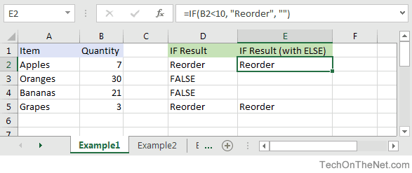
Based on the Excel spreadsheet above, the following IF examples would return:
=IF(B2<10, "Reorder", "")
Result: "Reorder"

=IF(A2="Apples", "Equal", "Not Equal")
Result: "Equal"

=IF(B3>=20, 12, 0)
Result: 12
Combining the IF function with Other Logical Functions
Quite often, you will need to specify more complex conditions when writing your formula in Excel. You can combine the IF function with other logical functions such as AND, OR, etc. Let’s explore this further.
AND function
The IF function can be combined with the AND function to allow you to test for multiple conditions. When using the AND function, all conditions within the AND function must be TRUE for the condition to be met. This comes in very handy in Excel formulas.
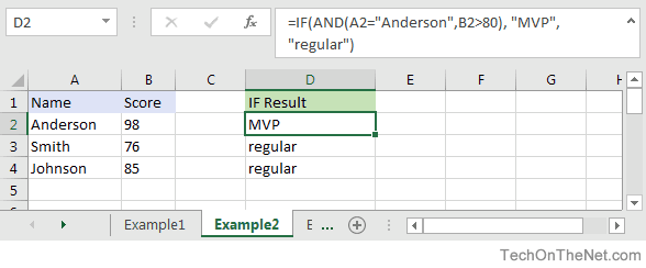
Based on the spreadsheet above, you can combine the IF function with the AND function as follows:
=IF(AND(A2="Anderson",B2>80), "MVP", "regular")
Result: "MVP"

=IF(AND(B2>=80,B2<=100), "Great Score", "Not Bad")
Result: "Great Score"

=IF(AND(B3>=80,B3<=100), "Great Score", "Not Bad")
Result: "Not Bad"

=IF(AND(A2="Anderson",A3="Smith",A4="Johnson"), 100, 50)
Result: 100

=IF(AND(A2="Anderson",A3="Smith",A4="Parker"), 100, 50)
Result: 50
In the examples above, all conditions within the AND function must be TRUE for the condition to be met.
OR function
The IF function can be combined with the OR function to allow you to test for multiple conditions. But in this case, only one or more of the conditions within the OR function needs to be TRUE for the condition to be met.
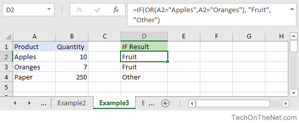
Based on the spreadsheet above, you can combine the IF function with the OR function as follows:
=IF(OR(A2="Apples",A2="Oranges"), "Fruit", "Other")
Result: "Fruit"

=IF(OR(A4="Apples",A4="Oranges"),"Fruit","Other")
Result: "Other"

=IF(OR(A4="Bananas",B4>=100), 999, "N/A")
Result: 999

=IF(OR(A2="Apples",A3="Apples",A4="Apples"), "Fruit", "Other")
Result: "Fruit"
In the examples above, only one of the conditions within the OR function must be TRUE for the condition to be met.
Let’s take a look at one more example that involves ranges of percentages.
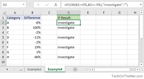
Based on the spreadsheet above, we would have the following formula in cell D2:
=IF(OR(B2>=5%,B2<=-5%),"investigate","")
Result: "investigate"
This IF function would return «investigate» if the value in cell B2 was either below -5% or above 5%. Since -6% is below -5%, it will return «investigate» as the result. We have copied this formula into cells D3 through D9 to show you the results that would be returned.
For example, in cell D3, we would have the following formula:
=IF(OR(B3>=5%,B3<=-5%),"investigate","")
Result: "investigate"
This formula would also return «investigate» but this time, it is because the value in cell B3 is greater than 5%.
Frequently Asked Questions
Question: In Microsoft Excel, I’d like to use the IF function to create the following logic:
if C11>=620, and C10=»F»or»S», and C4<=$1,000,000, and C4<=$500,000, and C7<=85%, and C8<=90%, and C12<=50, and C14<=2, and C15=»OO», and C16=»N», and C19<=48, and C21=»Y», then reference cell A148 on Sheet2. Otherwise, return an empty string.
Answer: The following formula would accomplish what you are trying to do:
=IF(AND(C11>=620, OR(C10="F",C10="S"), C4<=1000000, C4<=500000, C7<=0.85, C8<=0.9, C12<=50, C14<=2, C15="OO", C16="N", C19<=48, C21="Y"), Sheet2!A148, "")
Question: In Microsoft Excel, I’m trying to use the IF function to return 0 if cell A1 is either < 150,000 or > 250,000. Otherwise, it should return A1.
Answer: You can use the OR function to perform an OR condition in the IF function as follows:
=IF(OR(A1<150000,A1>250000),0,A1)
In this example, the formula will return 0 if cell A1 was either less than 150,000 or greater than 250,000. Otherwise, it will return the value in cell A1.
Question: In Microsoft Excel, I’m trying to use the IF function to return 25 if cell A1 > 100 and cell B1 < 200. Otherwise, it should return 0.
Answer: You can use the AND function to perform an AND condition in the IF function as follows:
=IF(AND(A1>100,B1<200),25,0)
In this example, the formula will return 25 if cell A1 is greater than 100 and cell B1 is less than 200. Otherwise, it will return 0.
Question: In Microsoft Excel, I need to write a formula that works this way:
IF (cell A1) is less than 20, then times it by 1,
IF it is greater than or equal to 20 but less than 50, then times it by 2
IF its is greater than or equal to 50 and less than 100, then times it by 3
And if it is great or equal to than 100, then times it by 4
Answer: You can write a nested IF statement to handle this. For example:
=IF(A1<20, A1*1, IF(A1<50, A1*2, IF(A1<100, A1*3, A1*4)))
Question: In Microsoft Excel, I need a formula in cell C5 that does the following:
IF A1+B1 <= 4, return $20
IF A1+B1 > 4 but <= 9, return $35
IF A1+B1 > 9 but <= 14, return $50
IF A1+B1 >= 15, return $75
Answer: In cell C5, you can write a nested IF statement that uses the AND function as follows:
=IF((A1+B1)<=4,20,IF(AND((A1+B1)>4,(A1+B1)<=9),35,IF(AND((A1+B1)>9,(A1+B1)<=14),50,75)))
Question: In Microsoft Excel, I need a formula that does the following:
IF the value in cell A1 is BLANK, then return «BLANK»
IF the value in cell A1 is TEXT, then return «TEXT»
IF the value in cell A1 is NUMERIC, then return «NUM»
Answer: You can write a nested IF statement that uses the ISBLANK function, the ISTEXT function, and the ISNUMBER function as follows:
=IF(ISBLANK(A1)=TRUE,"BLANK",IF(ISTEXT(A1)=TRUE,"TEXT",IF(ISNUMBER(A1)=TRUE,"NUM","")))
Question: In Microsoft Excel, I want to write a formula for the following logic:
IF R1<0.3 AND R2<0.3 AND R3<0.42 THEN «OK» OTHERWISE «NOT OK»
Answer: You can write an IF statement that uses the AND function as follows:
=IF(AND(R1<0.3,R2<0.3,R3<0.42),"OK","NOT OK")
Question: In Microsoft Excel, I need a formula for the following:
IF cell A1= PRADIP then value will be 100
IF cell A1= PRAVIN then value will be 200
IF cell A1= PARTHA then value will be 300
IF cell A1= PAVAN then value will be 400
Answer: You can write an IF statement as follows:
=IF(A1="PRADIP",100,IF(A1="PRAVIN",200,IF(A1="PARTHA",300,IF(A1="PAVAN",400,""))))
Question: In Microsoft Excel, I want to calculate following using an «if» formula:
if A1<100,000 then A1*.1% but minimum 25
and if A1>1,000,000 then A1*.01% but maximum 5000
Answer: You can write a nested IF statement that uses the MAX function and the MIN function as follows:
=IF(A1<100000,MAX(25,A1*0.1%),IF(A1>1000000,MIN(5000,A1*0.01%),""))
Question: In Microsoft Excel, I am trying to create an IF statement that will repopulate the data from a particular cell if the data from the formula in the current cell equals 0. Below is my attempt at creating an IF statement that would populate the data; however, I was unsuccessful.
=IF(IF(ISERROR(M24+((L24-S24)/AA24)),"0",M24+((L24-S24)/AA24)))=0,L24)
The initial part of the formula calculates the EAC (Estimate At completion = AC+(BAC-EV)/CPI); however if the current EV (Earned Value) is zero, the EAC will equal zero. IF the outcome is zero, I would like the BAC (Budget At Completion), currently recorded in another cell (L24), to be repopulated in the current cell as the EAC.
Answer: You can write an IF statement that uses the OR function and the ISERROR function as follows:
=IF(OR(S24=0,ISERROR(M24+((L24-S24)/AA24))),L24,M24+((L24-S24)/AA24))
Question: I have been looking at your Excel IF, AND and OR sections and found this very helpful, however I cannot find the right way to write a formula to express if C2 is either 1,2,3,4,5,6,7,8,9 and F2 is F and F3 is either D,F,B,L,R,C then give a value of 1 if not then 0. I have tried many formulas but just can’t get it right, can you help please?
Answer: You can write an IF statement that uses the AND function and the OR function as follows:
=IF(AND(C2>=1,C2<=9, F2="F",OR(F3="D",F3="F",F3="B",F3="L",F3="R",F3="C")),1,0)
Question:In Excel, I have a roadspeed of a car in m/s in cell A1 and a drop down menu of different units in C1 (which unclude mph and kmh). I have used the following IF function in B1 to convert the number to the unit selected from the dropdown box:
=IF(C1="mph","=A1*2.23693629",IF(C1="kmh","A1*3.6"))
However say if kmh was selected B1 literally just shows A1*3.6 and does not actually calculate it. Is there away to get it to calculate it instead of just showing the text message?
Answer: You are very close with your formula. Because you are performing mathematical operations (such as A1*2.23693629 and A1*3.6), you do not need to surround the mathematical formulas in quotes. Quotes are necessary when you are evaluating strings, not performing math.
Try the following:
=IF(C1="mph",A1*2.23693629,IF(C1="kmh",A1*3.6))
Question:For an IF statement in Excel, I want to combine text and a value.
For example, I want to put an equation for work hours and pay. IF I am paid more than I should be, I want it to read how many hours I owe my boss. But if I work more than I am paid for, I want it to read what my boss owes me (hours*Pay per Hour).
I tried the following:
=IF(A2<0,"I owe boss" abs(A2) "Hours","Boss owes me" abs(A2)*15 "dollars")
Is it possible or do I have to do it in 2 separate cells? (one for text and one for the value)
Answer: There are two ways that you can concatenate text and values. The first is by using the & character to concatenate:
=IF(A2<0,"I owe boss " & ABS(A2) & " Hours","Boss owes me " & ABS(A2)*15 & " dollars")
Or the second method is to use the CONCATENATE function:
=IF(A2<0,CONCATENATE("I owe boss ", ABS(A2)," Hours"), CONCATENATE("Boss owes me ", ABS(A2)*15, " dollars"))
Question:I have Excel 2000. IF cell A2 is greater than or equal to 0 then add to C1. IF cell B2 is greater than or equal to 0 then subtract from C1. IF both A2 and B2 are blank then equals C1. Can you help me with the IF function on this one?
Answer: You can write a nested IF statement that uses the AND function and the ISBLANK function as follows:
=IF(AND(ISBLANK(A2)=FALSE,A2>=0),C1+A2, IF(AND(ISBLANK(B2)=FALSE,B2>=0),C1-B2, IF(AND(ISBLANK(A2)=TRUE, ISBLANK(B2)=TRUE),C1,"")))
Question:How would I write this equation in Excel? IF D12<=0 then D12*L12, IF D12 is > 0 but <=600 then D12*F12, IF D12 is >600 then ((600*F12)+((D12-600)*E12))
Answer: You can write a nested IF statement as follows:
=IF(D12<=0,D12*L12,IF(D12>600,((600*F12)+((D12-600)*E12)),D12*F12))
Question:In Excel, I have this formula currently:
=IF(OR(A1>=40, B1>=40, C1>=40), "20", (A1+B1+C1)-20)
If one of my salesman does sale for $40-$49, then his commission is $20; however if his/her sale is less (for example $35) then the commission is that amount minus $20 ($35-$20=$15). I have 3 columns that are needed based on the type of sale. Only one column per row will be needed. The problem is that, when left blank, the total in the formula cell is -20. I need help setting up this formula so that when the 3 columns are left blank, the cell with the formula is left blank as well.
Answer: Using the AND function and the ISBLANK function, you can write your IF statement as follows:
=IF(AND(ISBLANK(A1),ISBLANK(B1),ISBLANK(C1)),"",IF(OR(A1>40, B1>40, C1>40), "20", (A1+B1+C1)-20))
In this formula, we are using the ISBLANK function to check if all 3 cells A1, B1, and C1 are blank, and if they are return a blank value («»). Then the rest is the formula that you originally wrote.
Question:In Excel, I need to create a simple booking and and out system, that shows a date out and a date back
«A1» = allows person to input date booked out
«A2» =allows person to input date booked back in
«A3″= shows status of product, eg, booked out, overdue return etc.
I can automate A3 with the following IF function:
=IF(ISBLANK(A2),"booked out","returned")
But what I cant get to work is if the product is out for 10 days or more, I would like the cell to say «send email»
Can you assist?
Answer: Using the TODAY function and adding an additional IF function, you can write your formula as follows:
=IF(ISBLANK(A2),IF(TODAY()-A1>10,"send email","booked out"),"returned")
Question:Using Microsoft Excel, I need a formula in cell U2 that does the following:
IF the date in E2<=12/31/2010, return T2*0.75
IF the date in E2>12/31/2010 but <=12/31/2011, return T2*0.5
IF the date in E2>12/31/2011, return T2*0
I tried using the following formula, but it gives me «#VALUE!»
=IF(E2<=DATE(2010,12,31),T2*0.75), IF(AND(E2>DATE(2010,12,31),E2<=DATE(2011,12,31)),T2*0.5,T2*0)
Can someone please help? Thanks.
Answer: You were very close…you just need to adjust your parentheses as follows:
=IF(E2<=DATE(2010,12,31),T2*0.75, IF(AND(E2>DATE(2010,12,31),E2<=DATE(2011,12,31)),T2*0.5,T2*0))
Question:In Excel, I would like to add 60 days if grade is ‘A’, 45 days if grade is ‘B’ and 30 days if grade is ‘C’. It would roughly look something like this, but I’m struggling with commas, brackets, etc.
(IF C5=A)=DATE(YEAR(B5)+0,MONTH(B5)+0,DAY(B5)+60),
(IF C5=B)=DATE(YEAR(B5)+0,MONTH(B5)+0,DAY(B5)+45),
(IF C5=C)=DATE(YEAR(B5)+0,MONTH(B5)+0,DAY(B5)+30)
Answer:You should be able to achieve your date calculations with the following formula:
=IF(C5="A",B5+60,IF(C5="B",B5+45,IF(C5="C",B5+30)))
Question:In Excel, I am trying to write a function and can’t seem to figure it out. Could you help?
IF D3 is < 31, then 1.51
IF D3 is between 31-90, then 3.40
IF D3 is between 91-120, then 4.60
IF D3 is > 121, then 5.44
Answer:You can write your formula as follows:
=IF(D3>121,5.44,IF(D3>=91,4.6,IF(D3>=31,3.4,1.51)))
Question:I would like ask a question regarding the IF statement. How would I write in Excel this problem?
I have to check if cell A1 is empty and if not, check if the value is less than equal to 5. Then multiply the amount entered in cell A1 by .60. The answer will be displayed on Cell A2.
Answer:You can write your formula in cell A2 using the IF function and ISBLANK function as follows:
=IF(AND(ISBLANK(A1)=FALSE,A1<=5),A1*0.6,"")
Question:In Excel, I’m trying to nest an OR command and I can’t find the proper way to write it. I want the spreadsheet to do the following:
If D6 equals «HOUSE» and C6 equals either «MOUSE» or «CAT», I want to return the value in cell B6. Otherwise, the formula should return the value «BLANK».
I tried the following:
=IF((D6="HOUSE")*(C6="MOUSE")*OR(C6="CAT"));B6;"BLANK")
If I only ask for HOUSE and MOUSE or HOUSE and CAT, it works, but as soon as I ask for MOUSE OR CAT, it doesn’t work.
Answer:You can write your formula using the AND function and OR function as follows:
=IF(AND(D6="HOUSE",OR(C6="MOUSE",C6="CAT")),B6,"BLANK")
This will return the value in B6 if D6 equals «HOUSE» and C6 equals either «MOUSE» or «CAT». If those conditions are not met, the formula will return the text value of «BLANK».
Question:In Microsoft Excel, I’m trying to write the following formula:
If cell A1 equals «jaipur», «udaipur» or «jodhpur», then cell A2 should display «rajasthan»
If cell A1 equals «bangalore», «mysore» or «belgum», then cell A2 should display «karnataka»
Please help.
Answer:You can write your formula using the OR function as follows:
=IF(OR(A1="jaipur",A1="udaipur",A1="jodhpur"),"rajasthan", IF(OR(A1="bangalore",A1="mysore",A1="belgum"),"karnataka"))
This will return «rajasthan» if A1 equals either «jaipur», «udaipur» or «jodhpur» and it will return «karnataka» if A1 equals either «bangalore», «mysore» or «belgum».
Question:In Microsoft Excel I’m trying to achieve the following with IF function:
If a value in any cell in column F is «food» then add the value of its corresponding cell in column G (eg a corresponding cell for F3 is G3). The IF function is performed in another cell altogether. I can do it for a single pair of cells but I don’t know how to do it for an entire column. Could you help?
At the moment, I’ve got this:
=IF(F3="food"; G3; 0)
Answer:This formula can be created using the SUMIF formula instead of using the IF function:
=SUMIF(F1:F10,"=food",G1:G10)
This will evaluate the first 10 rows of data in your spreadsheet. You may need to adjust the ranges accordingly.
I notice that you separate your parameters with semi-colons, so you might need to replace the commas in the formula above with semi-colons.
Question:I’m looking for an Exel formula that says:
If F3 is «H» and E3 is «H», return 1
If F3 is «A» and E3 is «A», return 2
If F3 is «d» and E3 is «d», return 3
Appreciate if you can help.
Answer:This Excel formula can be created using the AND formula in combination with the IF function:
=IF(AND(F3="H",E3="H"),1,IF(AND(F3="A",E3="A"),2,IF(AND(F3="d",E3="d"),3,"")))
We’ve defaulted the formula to return a blank if none of the conditions above are met.
Question:I am trying to get Excel to check different boxes and check if there is text/numbers listed in the cells and then spit out «Complete» if all 5 Boxes have text/Numbers or «Not Complete» if one or more is empty. This is what I have so far and it doesn’t work.
=IF(OR(ISBLANK(J2),ISBLANK(M2),ISBLANK(R2),ISBLANK (AA2),ISBLANK (AB2)),"Not Complete","")
Answer:First, you are correct in using the ISBLANK function, however, you have a space between ISBLANK and (AA2), as well as ISBLANK and (AB2). This might seem insignificant, but Excel can be very picky and will return a #NAME? error. So first you need to eliminate those spaces.
Next, you need to change the ELSE condition of your IF function to return «Complete».
You should be able to modify your formula as follows:
=IF(OR(ISBLANK(J2),ISBLANK(M2),ISBLANK(R2),ISBLANK(AA2),ISBLANK(AB2)), "Not Complete", "Complete")
Now if any of the cell J2, M2, R2, AA2, or AB2 are blank, the formula will return «Not Complete». If all 5 cells have a value, the formula will return «Complete».
Question:I’m very new to the Excel world, and I’m trying to figure out how to set up the proper formula for an If/then cell.
What I’m trying for is:
If B2’s value is 1 to 5, then multiply E2 by .77
If B2’s value is 6 to 10, then multiply E2 by .735
If B2’s value is 11 to 19, then multiply E2 by .7
If B2’s value is 20 to 29, then multiply E2 by .675
If B2’s value is 30 to 39, then multiply E2 by .65
I’ve tried a few different things thinking I was on the right track based on the IF, and AND function tutorials here, but I can’t seem to get it right.
Answer:To write your IF formula, you need to nest multiple IF functions together in combination with the AND function.
The following formula should work for what you are trying to do:
=IF(AND(B2>=1, B2<=5), E2*0.77, IF(AND(B2>=6, B2<=10), E2*0.735, IF(AND(B2>=11, B2<=19), E2*0.7, IF(AND(B2>=20, B2<=29), E2*0.675, IF(AND(B2>=30, B2<=39), E2*0.65,"")))))
As one final component of your formula, you need to decide what to do when none of the conditions are met. In this example, we have returned «» when the value in B2 does not meet any of the IF conditions above.
Question:Here is the Excel formula that has me between a rock and a hard place.
If E45 <= 50, return 44.55
If E45 > 50 and E45 < 100, return 42
If E45 >=200, return 39.6
Again thank you very much.
Answer:You should be able to write this Excel formula using a combination of the IF function and the AND function.
The following formula should work:
=IF(E45<=50, 44.55, IF(AND(E45>50, E45<100), 42, IF(E45>=200, 39.6, "")))
Please note that if none of the conditions are met, the Excel formula will return «» as the result.
Question:I have a nesting OR function problem:
My nonworking formula is:
=IF(C9=1,K9/J7,IF(C9=2,K9/J7,IF(C9=3,K9/L7,IF(C9=4,0,K9/N7))))
In Cell C9, I can have an input of 1, 2, 3, 4 or 0. The problem is on how to write the «or» condition when a «4 or 0» exists in Column C. If the «4 or 0» conditions exists in Column C I want Column K divided by Column N and the answer to be placed in Column M and associated row
Answer:You should be able to use the OR function within your IF function to test for C9=4 OR C9=0 as follows:
=IF(C9=1,K9/J7,IF(C9=2,K9/J7,IF(C9=3,K9/L7,IF(OR(C9=4,C9=0),K9/N7))))
This formula will return K9/N7 if cell C9 is either 4 or 0.
Question:In Excel, I am trying to create a formula that will show the following:
If column B = Ross and column C = 8 then in cell AB of that row I want it to show 2013, If column B = Block and column C = 9 then in cell AB of that row I want it to show 2012.
Answer:You can create your Excel formula using nested IF functions with the AND function.
=IF(AND(B1="Ross",C1=8),2013,IF(AND(B1="Block",C1=9),2012,""))
This formula will return 2013 as a numeric value if B1 is «Ross» and C1 is 8, or 2012 as a numeric value if B1 is «Block» and C1 is 9. Otherwise, it will return blank, as denoted by «».
Question:In Excel, I really have a problem looking for the right formula to express the following:
If B1=0, C1 is equal to A1/2
If B1=1, C1 is equal to A1/2 times 20%
If D1=1, C1 is equal to A1/2-5
I’ve been trying to look for any same expressions in your site. Please help me fix this.
Answer:In cell C1, you can use the following Excel formula with 3 nested IF functions:
=IF(B1=0,A1/2, IF(B1=1,(A1/2)*0.2, IF(D1=1,(A1/2)-5,"")))
Please note that if none of the conditions are met, the Excel formula will return «» as the result.
Question:In Excel, I need the answer for an IF THEN statement which compares column A and B and has an «OR condition» for column C. My problem is I want column D to return yes if A1 and B1 are >=3 or C1 is >=1.
Answer:You can create your Excel IF formula as follows:
=IF(OR(AND(A1>=3,B1>=3),C1>=1),"yes","")
Please note that if none of the conditions are met, the Excel formula will return «» as the result.
Question:In Excel, what have I done wrong with this formula?
=IF(OR(ISBLANK(C9),ISBLANK(B9)),"",IF(ISBLANK(C9),D9-TODAY(), "Reactivated"))
I want to make an event that if B9 and C9 is empty, the value would be empty. If only C9 is empty, then the output would be the remaining days left between the two dates, and if the two cells are not empty, the output should be the string ‘Reactivated’.
The problem with this code is that IF(ISBLANK(C9),D9-TODAY() is not working.
Answer:First of all, you might want to replace your OR function with the AND function, so that your Excel IF formula looks like this:
=IF(AND(ISBLANK(C9),ISBLANK(B9)),"",IF(ISBLANK(C9),D9-TODAY(),"Reactivated"))
Next, make sure that you don’t have any abnormal formatting in the cell that contains the results. To be safe, right click on the cell that contains the formula and choose Format Cells from the popup menu. When the Format Cells window appears, select the Number tab. Choose General as the format and click on the OK button.
Question:I was wondering if you could tell me what I am doing wrong.
Here are the instructions:
A customer is eligible for a discount if the customer’s 2016 sales greater than or equal to 100000 OR if the customers First Order was placed in 2016.
If the customer qualifies for a discount, return a value of Y
If the customer does not qualify for a discount, return a value of N.
Here is the formula I’ve entered:
=IF(OR([2014 Sales]=0,[2015 Sales]=0,[2016 Sales]>=100000),"Y","N")
I only have 2 cells wrong. Can you help me please? I am very lost and confused.
Answer:You are very close with your IF formula, however, it looks like you need to add the AND function to your formula as follows:
=IF(OR([2016 Sales]>=100000,AND([2014 Sales]=0,[2015 Sales]=0),C8>=100000),"Y","N")
This formula should return Y if 2016 sales are greater than or equal to 100000, or if both 2014 sales and 2015 sales are 0. Otherwise, the formula will return N. You will also notice that we switched the order of your conditions in the formula so that it is easier to understand the formula based on your instructions above.
Question:Could you please help me? I need to use «OR» on my formula but I can’t get it to work. This is what I’ve tried:
=IF(C6>=0<=150,150000,IF(C6>=151<=160,158400))
Here is what I need the formula to do:
IF C6 IS >=0 OR <=150 THEN ASSIGN $150000
IF C6 IS >=151 OR <=160 THEN ASSIGN $158400
Answer:You should be able to use the AND function within your IF function as follows:
=IF(AND(ISBLANK(C6)=FALSE,C6>=0,C6<=150),150000,IF(AND(C6>=151,C6<=160),158400,""))
Notice that we first use the ISBLANK function to test C6 to make sure that it is not blank. This is because if C6 if blank, it will evalulate to greater than 0 and thus return 150000. To avoid this, we include ISBLANK(C6)=FALSE as one of the conditions in addition to C6>=0 and C6<=150. That way, you won’t return any false results if C6 is blank.
Question:I am having a problem with a formula, I want it to be IF E5=N then do the first formula, else do the second formula. Excel recognizes the =IF(logical_test,value_if_TRUE,value_if_FALSE) but doesn’t like the formula below:
=IF(e5="N",((AND(AH5-AG5<456, AH5-S5<822)), "Compliant", "not Compliant"),((AH5-S5<822), "Compliant", "not Compliant"))
Any help would be greatly appreciated.
Answer:To have the first formula executed when E5=N and then second formula executed when E5<>N, you will need to nest 2 additional IF functions within the main IF function as follows:
=IF(E5="N", IF((AND(AH5-AG5<456, AH5-S5<822)), "Compliant", "not Compliant"), IF((AH5-S5<822), "Compliant", "not Compliant"))
If E5=»N», the first nested IF function will be executed:
IF((AND(AH5-AG5<456, AH5-S5<822)), "Compliant", "not Compliant")
Otherwise,the second nested IF function will be executed:
IF((AH5-S5<822), "Compliant", "not Compliant"))
Question:I need to write a formula based on the following logic:
There is a maximum discount allowed of £1000 if the capital sum is less that £43000 and a lower discount of £500 if the capital sum is above £43000. So the formula should return either £500 or £1000 in the cell but the £43000 is made up of two numbers, say for e.g. £42750+350 and if the second number is less than the allowed discount, the actual lower value is returned — in this case the £500 or £1000 becomes £350. Or as another e.g. £42000+750 returns £750.
So on my spreadsheet, in this second e.g. I would have A1= £42000, A2=750, A3=A1+A2, A4=the formula with the changing discount, in this case £750.
How can I write this formula?
Answer:In cell A4, you can calculate the correct discount using the IF function and the MIN function as follows:
=IF(A3<43000, MIN(A2,1000), MIN(A2,500))
If A3 is less than 43000, the formula will return the lower value of A2 and 1000. Otherwise, it will return the lower value of A2 and 500.
Question: I have a list of sizes in column A with sizes 100, 200, 300, 400, 500, 600. Then I have another column B, with sizes of my products, and it is random, for example, 318, 445, 527. What I’m trying to create is for a value of 318 in column B, I need to return 400 for that product. If the value in column B is 445, then I should return 500 and so on, as long sizes in column A must be BIGGER to the NEAREST size to column B.
Any idea how to create this function?
Answer:If your sizes are in increments of 100, you can create this function by taking the value in column B, dividing by 100, rounding up to the nearest integer, and then multiplying by 100.
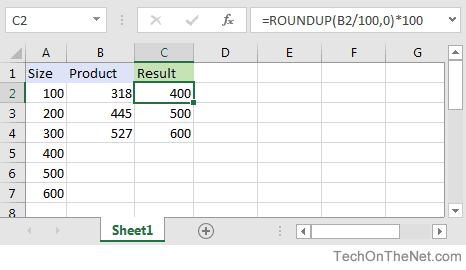
For example in cell C2, you can use the IF function and the ROUNDUP function as follows:
=ROUNDUP(B2/100,0)*100
This will return the correct value of 400 for a value of 318 in cell B2. Just copy this formula to cell C3, C4 and so on.
The IF function is one of the most commonly used in Excel. The function can test a single condition as well as perform multiple complex logic tests. We can thus control the execution of Excel tasks using the IF function.
This is important since it enables us to perform actions depending on whether they meet certain conditions defined by the IF formula. We can also add data to cells using the function if other cells meet any of the conditions defined in the IF formula.
To add multiple conditions to an IF formula, we simply add nested IF functions.
In this article, you will learn the basics of the IF function and how to come up with an array of IF formulas. You will also learn the nested IF’s function.
Let’s get started!
1. Basic IF formula that tests a single condition
A single IF statement tests whether a condition is met and returns a value if TRUE and another value if FALSE.
IF (logical test, ‘value_if_true’, ‘value_if_false’)
In the example below, let us test whether the price is less than or equal to 2000. If the condition is true return cheap, otherwise return expensive!
Go to Cell C2 and type ‘=IF(B2<=2000,»CHEAP», «EXPENSIVE»)’

The if formula above records or posts the String Good whenever the single condition B2<=2000.
2. IF formula with multiple conditions (Nested IF Functions.
If you have complex data or want to perform powerful data analysis, you might need to test multiple conditions at a time. You might need to perform a logical test across multiple conditions.
In such cases, you have to use an IF statement with multiple conditions/ranges in a single formula. These multiple IF conditions are normally called nested IF Functions. The function is used if want more than 3 different results.
The general syntax for IF function with multiple conditions is
=IF (condition one is true, do something, IF (condition two is true, do something, IF (conditions three is true, do something, else do something)))
Commas are used to separate conditions and IF functions in the IF formula. The «)» is used to close all IFs at the End of the formula while the » (» opens all IF functions. The number of «(» should be equal to that of «)».
In our above example, we can include multiple conditions in the IF formula as follows
=IF(B2<=2000,»CHEAP»,IF(B2<=6000,»AFFORDABLE»,IF(B2<=10000,»EXPENSIVE»,»LUXURIOUS»)))

Press Enter to get the results and use the AutoFill feature to copy the formula to the rest of the cells.

3. IF formula with logical test
You can use an IF statement with AND and OR conditions to perform a logical test. IF your formula has AND function, the logical test returns TRUE if all the conditions are met; otherwise, it will return FALSE. While the OR Function returns TRUE if any of the conditions is met; otherwise it returns FALSE.
3.1 IF with AND Function
In the example below, a student is deemed to pass the exam if he/she has a score of 42 in Maths and 50 in English.

With this information, we can write the condition as follows;
AND (C14>=42, D14>=50)
To know whether the student passed or failed the exam. You can use the IF statement.
= IF(AND (C14>=42, D14>=50),”PASS”,”FAIL”)

Press enter and use the AutoFill feature to copy the formula to the rest of the cells.

3.2 IF with OR Function
The IF with OR Function works the same way as the AND function we have seen above. The only difference is that, if one of the conditions is TRUE then the result will be TRUE.
Follow the above process to apply the OR Function.
In cell E14, type = IF(OR (C14>=42, D14>=50),”PASS”,”FAIL”)

Press enter to get the results.

3. IF with ISNUMBER and ISTEXT Functions
You can use ISNUMBER and ISTEXT formula to find whether the cells have text value, number, or blank.
=IF(ISTEXT(A1), «Text», IF(ISNUMBER(A1), «Number», IF(ISBLANK(A1), «Blank», «»)))

You can only apply AND & OR functions at a time if your task requires you to evaluate several sets of conditions. For example, if you are checking exam results using these criteria:
Condition 1: exam1>50 and exam2>50
Condition 2: exam1>40 and exam2>60
In this case, the exam is deemed passed if either of the conditions is passed.
Although the formula may seem tricky, you only need to express each condition as an AND statement and nest them in the OR function. That is because meeting all the conditions is not necessary, but either statement will serve the purpose. Therefore, the general formula will be:
OR(AND(B2>50, C2>50), AND(B2>40, C2>60)
You can now use the OR function to test the logic of IF and supply the desired value_if_true and value_if_false values. In the end, the final IF formula with multiple AND & OR statements will turn into:
=IF(OR(AND(B2>50, C2>50), AND(B2>40, C2>60), «Pass», «Fail»)


5. Using the Array Formula
An Array formula can also help to get an Excel IF to test multiple conditions. For example, to evaluate the AND logical condition, you can use the asterisk:
IF(condition1) * (condition2) * …, value_if_true, value_if_false)
While to test conditions using OR logic, you will apply the plus sign:
IF(condition1) + (condition2) + …, value_if_true, value_if_false)
Finally, you can complete the Array formula by pressing Ctrl + Shift + Enter buttons together. The trick can also work as a regular formula in Excel 365 and Excel 2021 since it supports dynamic arrays.
Example: We can get “Pass” if cells B2 and C2 are greater than 50 by applying the formulas;
=IF((B2>50) * (C2>50), «Pass», «Fail») for AND logic


…, and
=IF((B2>50) + (C2>50), «Pass», «Fail») for OR logic.


6. IF With Other Excel Functions
Other Excel functions that can give the IF formula for multiple conditions include
6.1 IF#N/A Error in VLOOKUP Function
The VLOOKUP or any other lookup function returns a N/A error if it cannot find something. Therefore, you can return zero, blank, or text if #N/A to make your table neat. Here, you will need the following generic formula:
IF(ISNA(VLOOKUP(…)), value_if_na, VLOOKUP(…))
Example 1. If the lookup value in a cell (E1) is not found, the formula returns 0 as shown below;
=IF(ISNA(VLOOKUP(E1, A2:B10, 2,FALSE )), 0, VLOOKUP(E1, A2:B10, 2, FALSE))

Example 2: If the lookup value is not found, the formula returns blank as shown below;
=IF(ISNA(VLOOKUP(E1, A2:B10, 2,FALSE )), «», VLOOKUP(E1, A2:B10, 2, FALSE))

Example 3: If the lookup value is not available, the formula returns a specific text as shown below;
=IF(ISNA(VLOOKUP(E1, A2:B10, 2,FALSE )), «Not found», VLOOKUP(E1, A2:B10, 2, FALSE))

6.2 IF With SUM, AVERAGE, MIN, and MAX Functions
Excel has the SUMIF and SUMIFS functions that you can use, to sum up values in cells using certain criteria. You can use the SUM function to test the IF logic of your business. For instance, you can apply this formula to determine the text labels based on the sum of cells B2 and C2 values;
=IF(SUM(B2:C2)>130, «Good», IF(SUM(B2:C2)>110, «Satisfactory», «Poor»))

From the formula, the return text label is “Good” if the sum of the two cells is greater than 130. If the sum is greater than 110, the return text is “Satisfactory”, while if the sum is 110 or below, the return text is “Poor”.
You can still embed the AVERAGE function similarly to test the IF logic and return a different text label based on the average score of the two cells. In this case, the generic formula will be;
=IF(AVERAGE(B2:C2)>65, «Good», IF(AVERAGE(B2:C2)>55, «Satisfactory», «Poor»))

If the sum of cells B2 and C2 is indicated in cell D2, you can use the MAX and MIN functions to identify the highest and lowest values through the formulas;
=IF(D2=MAX($D$2: $D$10), «Best result», «»)

=IF(D2=MAX($D$2: $D$10), «Best result», «»)

Lastly, you can nest the two functions into one another to have both text labels in one column to get the formula;
=IF(D2=MAX($D$2:$D$10), «Best result», IF(D2=MIN($D$2:$D$10), «Worst result», «»))

6.3 IF with CONCATENATE Function
You can also use the CONCATENATE and IF functions to output the result of IF and some text into one cell. Here, you can use the formula;
=CONCATENATE(«You performed «, IF(B1>100,»fantastic!», IF(B1>50, «well», «poor»)))

From the formula, the student will get a «fantastic» result if the score in cell B1 is greater than 100. On the other hand, the result will be «well» if the score in cell B1 is greater than 50.
6.4 IF with ISERROR and ISNA Functions
These functions can only work in modern Excel versions where they trap and replace errors with another predefined value. For instance, the IFERROR function works in Excel 2007 and later, while the IFNA function works in Excel 2013 and later. When using earlier Excel versions, you will need the combinations of IF ISERROR and IF ISNA. So, what is the difference between these applications?
The answer is simple: IFERROR and ISERROR functions can handle all the possible errors resulting from Excel calculations, including VALUE, N/A, NAME, REF, NUM, DIV/0, and NULL errors. Contrary, IFNA, and ISNA handle only N/A errors.
Example: If you want to replace the #DIV/0 (divide by zero error) with a predefined text or value, you can use the formula;
=IF(ISERROR(A2/B2), «N/A», A2/B2), where;
A2 represents the value in cell A2
B2 represents the value in cell B2.
A2/B2 represents the results attained after dividing A2 by B2.
If the value in cell B2 is 0, the formula will return a N/A text.

I hope you found this tutorial useful.