
The IF function allows you to make a logical comparison between a value and what you expect by testing for a condition and returning a result if that condition is True or False.
-
=IF(Something is True, then do something, otherwise do something else)
But what if you need to test multiple conditions, where let’s say all conditions need to be True or False (AND), or only one condition needs to be True or False (OR), or if you want to check if a condition does NOT meet your criteria? All 3 functions can be used on their own, but it’s much more common to see them paired with IF functions.
Use the IF function along with AND, OR and NOT to perform multiple evaluations if conditions are True or False.
Syntax
-
IF(AND()) — IF(AND(logical1, [logical2], …), value_if_true, [value_if_false]))
-
IF(OR()) — IF(OR(logical1, [logical2], …), value_if_true, [value_if_false]))
-
IF(NOT()) — IF(NOT(logical1), value_if_true, [value_if_false]))
|
Argument name |
Description |
|
|
logical_test (required) |
The condition you want to test. |
|
|
value_if_true (required) |
The value that you want returned if the result of logical_test is TRUE. |
|
|
value_if_false (optional) |
The value that you want returned if the result of logical_test is FALSE. |
|
Here are overviews of how to structure AND, OR and NOT functions individually. When you combine each one of them with an IF statement, they read like this:
-
AND – =IF(AND(Something is True, Something else is True), Value if True, Value if False)
-
OR – =IF(OR(Something is True, Something else is True), Value if True, Value if False)
-
NOT – =IF(NOT(Something is True), Value if True, Value if False)
Examples
Following are examples of some common nested IF(AND()), IF(OR()) and IF(NOT()) statements. The AND and OR functions can support up to 255 individual conditions, but it’s not good practice to use more than a few because complex, nested formulas can get very difficult to build, test and maintain. The NOT function only takes one condition.

Here are the formulas spelled out according to their logic:
|
Formula |
Description |
|---|---|
|
=IF(AND(A2>0,B2<100),TRUE, FALSE) |
IF A2 (25) is greater than 0, AND B2 (75) is less than 100, then return TRUE, otherwise return FALSE. In this case both conditions are true, so TRUE is returned. |
|
=IF(AND(A3=»Red»,B3=»Green»),TRUE,FALSE) |
If A3 (“Blue”) = “Red”, AND B3 (“Green”) equals “Green” then return TRUE, otherwise return FALSE. In this case only the first condition is true, so FALSE is returned. |
|
=IF(OR(A4>0,B4<50),TRUE, FALSE) |
IF A4 (25) is greater than 0, OR B4 (75) is less than 50, then return TRUE, otherwise return FALSE. In this case, only the first condition is TRUE, but since OR only requires one argument to be true the formula returns TRUE. |
|
=IF(OR(A5=»Red»,B5=»Green»),TRUE,FALSE) |
IF A5 (“Blue”) equals “Red”, OR B5 (“Green”) equals “Green” then return TRUE, otherwise return FALSE. In this case, the second argument is True, so the formula returns TRUE. |
|
=IF(NOT(A6>50),TRUE,FALSE) |
IF A6 (25) is NOT greater than 50, then return TRUE, otherwise return FALSE. In this case 25 is not greater than 50, so the formula returns TRUE. |
|
=IF(NOT(A7=»Red»),TRUE,FALSE) |
IF A7 (“Blue”) is NOT equal to “Red”, then return TRUE, otherwise return FALSE. |
Note that all of the examples have a closing parenthesis after their respective conditions are entered. The remaining True/False arguments are then left as part of the outer IF statement. You can also substitute Text or Numeric values for the TRUE/FALSE values to be returned in the examples.
Here are some examples of using AND, OR and NOT to evaluate dates.

Here are the formulas spelled out according to their logic:
|
Formula |
Description |
|---|---|
|
=IF(A2>B2,TRUE,FALSE) |
IF A2 is greater than B2, return TRUE, otherwise return FALSE. 03/12/14 is greater than 01/01/14, so the formula returns TRUE. |
|
=IF(AND(A3>B2,A3<C2),TRUE,FALSE) |
IF A3 is greater than B2 AND A3 is less than C2, return TRUE, otherwise return FALSE. In this case both arguments are true, so the formula returns TRUE. |
|
=IF(OR(A4>B2,A4<B2+60),TRUE,FALSE) |
IF A4 is greater than B2 OR A4 is less than B2 + 60, return TRUE, otherwise return FALSE. In this case the first argument is true, but the second is false. Since OR only needs one of the arguments to be true, the formula returns TRUE. If you use the Evaluate Formula Wizard from the Formula tab you’ll see how Excel evaluates the formula. |
|
=IF(NOT(A5>B2),TRUE,FALSE) |
IF A5 is not greater than B2, then return TRUE, otherwise return FALSE. In this case, A5 is greater than B2, so the formula returns FALSE. |

Using AND, OR and NOT with Conditional Formatting
You can also use AND, OR and NOT to set Conditional Formatting criteria with the formula option. When you do this you can omit the IF function and use AND, OR and NOT on their own.
From the Home tab, click Conditional Formatting > New Rule. Next, select the “Use a formula to determine which cells to format” option, enter your formula and apply the format of your choice.

Using the earlier Dates example, here is what the formulas would be.

|
Formula |
Description |
|---|---|
|
=A2>B2 |
If A2 is greater than B2, format the cell, otherwise do nothing. |
|
=AND(A3>B2,A3<C2) |
If A3 is greater than B2 AND A3 is less than C2, format the cell, otherwise do nothing. |
|
=OR(A4>B2,A4<B2+60) |
If A4 is greater than B2 OR A4 is less than B2 plus 60 (days), then format the cell, otherwise do nothing. |
|
=NOT(A5>B2) |
If A5 is NOT greater than B2, format the cell, otherwise do nothing. In this case A5 is greater than B2, so the result will return FALSE. If you were to change the formula to =NOT(B2>A5) it would return TRUE and the cell would be formatted. |
Note: A common error is to enter your formula into Conditional Formatting without the equals sign (=). If you do this you’ll see that the Conditional Formatting dialog will add the equals sign and quotes to the formula — =»OR(A4>B2,A4<B2+60)», so you’ll need to remove the quotes before the formula will respond properly.
Need more help?

See also
You can always ask an expert in the Excel Tech Community or get support in the Answers community.
Learn how to use nested functions in a formula
IF function
AND function
OR function
NOT function
Overview of formulas in Excel
How to avoid broken formulas
Detect errors in formulas
Keyboard shortcuts in Excel
Logical functions (reference)
Excel functions (alphabetical)
Excel functions (by category)
Функция ЕСЛИ в Excel — это отличный инструмент для проверки условий на ИСТИНУ или ЛОЖЬ. Если значения ваших расчетов равны заданным параметрам функции как ИСТИНА, то она возвращает одно значение, если ЛОЖЬ, то другое.
Содержание
- Что возвращает функция
- Синтаксис
- Аргументы функции
- Дополнительная информация
- Функция Если в Excel примеры с несколькими условиями
- Пример 1. Проверяем простое числовое условие с помощью функции IF (ЕСЛИ)
- Пример 2. Использование вложенной функции IF (ЕСЛИ) для проверки условия выражения
- Пример 3. Вычисляем сумму комиссии с продаж с помощью функции IF (ЕСЛИ) в Excel
- Пример 4. Используем логические операторы (AND/OR) (И/ИЛИ) в функции IF (ЕСЛИ) в Excel
- Пример 5. Преобразуем ошибки в значения “0” с помощью функции IF (ЕСЛИ)
Что возвращает функция
Заданное вами значение при выполнении двух условий ИСТИНА или ЛОЖЬ.
Синтаксис
=IF(logical_test, [value_if_true], [value_if_false]) — английская версия
=ЕСЛИ(лог_выражение; [значение_если_истина]; [значение_если_ложь]) — русская версия
Аргументы функции
- logical_test (лог_выражение) — это условие, которое вы хотите протестировать. Этот аргумент функции должен быть логичным и определяемым как ЛОЖЬ или ИСТИНА. Аргументом может быть как статичное значение, так и результат функции, вычисления;
- [value_if_true] ([значение_если_истина]) — (не обязательно) — это то значение, которое возвращает функция. Оно будет отображено в случае, если значение которое вы тестируете соответствует условию ИСТИНА;
- [value_if_false] ([значение_если_ложь]) — (не обязательно) — это то значение, которое возвращает функция. Оно будет отображено в случае, если условие, которое вы тестируете соответствует условию ЛОЖЬ.
Дополнительная информация
- В функции ЕСЛИ может быть протестировано 64 условий за один раз;
- Если какой-либо из аргументов функции является массивом — оценивается каждый элемент массива;
- Если вы не укажете условие аргумента FALSE (ЛОЖЬ) value_if_false (значение_если_ложь) в функции, т.е. после аргумента value_if_true (значение_если_истина) есть только запятая (точка с запятой), функция вернет значение “0”, если результат вычисления функции будет равен FALSE (ЛОЖЬ).
На примере ниже, формула =IF(A1> 20,”Разрешить”) или =ЕСЛИ(A1>20;»Разрешить») , где value_if_false (значение_если_ложь) не указано, однако аргумент value_if_true (значение_если_истина) по-прежнему следует через запятую. Функция вернет “0” всякий раз, когда проверяемое условие не будет соответствовать условиям TRUE (ИСТИНА).
 |
| - Если вы не укажете условие аргумента TRUE(ИСТИНА) (value_if_true (значение_если_истина)) в функции, т.е. условие указано только для аргумента value_if_false (значение_если_ложь), то формула вернет значение “0”, если результат вычисления функции будет равен TRUE (ИСТИНА);
На примере ниже формула равна =IF (A1>20;«Отказать») или =ЕСЛИ(A1>20;»Отказать»), где аргумент value_if_true (значение_если_истина) не указан, формула будет возвращать “0” всякий раз, когда условие соответствует TRUE (ИСТИНА).

Функция Если в Excel примеры с несколькими условиями
Пример 1. Проверяем простое числовое условие с помощью функции IF (ЕСЛИ)
При использовании функции ЕСЛИ в Excel, вы можете использовать различные операторы для проверки состояния. Вот список операторов, которые вы можете использовать:
Ниже приведен простой пример использования функции при расчете оценок студентов. Если сумма баллов больше или равна «35», то формула возвращает “Сдал”, иначе возвращается “Не сдал”.
Пример 2. Использование вложенной функции IF (ЕСЛИ) для проверки условия выражения
Функция может принимать до 64 условий одновременно. Несмотря на то, что создавать длинные вложенные функции нецелесообразно, то в редких случаях вы можете создать формулу, которая множество условий последовательно.
В приведенном ниже примере мы проверяем два условия.
- Первое условие проверяет, сумму баллов не меньше ли она чем 35 баллов. Если это ИСТИНА, то функция вернет “Не сдал”;
- В случае, если первое условие — ЛОЖЬ, и сумма баллов больше 35, то функция проверяет второе условие. В случае если сумма баллов больше или равна 75. Если это правда, то функция возвращает значение “Отлично”, в других случаях функция возвращает “Сдал”.
Пример 3. Вычисляем сумму комиссии с продаж с помощью функции IF (ЕСЛИ) в Excel
Функция позволяет выполнять вычисления с числами. Хороший пример использования — расчет комиссии продаж для торгового представителя.
В приведенном ниже примере, торговый представитель по продажам:
- не получает комиссионных, если объем продаж меньше 50 тыс;
- получает комиссию в размере 2%, если продажи между 50-100 тыс
- получает 4% комиссионных, если объем продаж превышает 100 тыс.
Рассчитать размер комиссионных для торгового агента можно по следующей формуле:
=IF(B2<50,0,IF(B2<100,B2*2%,B2*4%)) — английская версия
=ЕСЛИ(B2<50;0;ЕСЛИ(B2<100;B2*2%;B2*4%)) — русская версия
В формуле, использованной в примере выше, вычисление суммы комиссионных выполняется в самой функции ЕСЛИ. Если объем продаж находится между 50-100K, то формула возвращает B2 * 2%, что составляет 2% комиссии в зависимости от объема продажи.
Больше лайфхаков в нашем Telegram Подписаться
Пример 4. Используем логические операторы (AND/OR) (И/ИЛИ) в функции IF (ЕСЛИ) в Excel
Вы можете использовать логические операторы (AND/OR) (И/ИЛИ) внутри функции для одновременного тестирования нескольких условий.
Например, предположим, что вы должны выбрать студентов для стипендий, основываясь на оценках и посещаемости. В приведенном ниже примере учащийся имеет право на участие только в том случае, если он набрал более 80 баллов и имеет посещаемость более 80%.
Вы можете использовать функцию AND (И) вместе с функцией IF (ЕСЛИ), чтобы сначала проверить, выполняются ли оба эти условия или нет. Если условия соблюдены, функция возвращает “Имеет право”, в противном случае она возвращает “Не имеет право”.
Формула для этого расчета:
=IF(AND(B2>80,C2>80%),”Да”,”Нет”) — английская версия
=ЕСЛИ(И(B2>80;C2>80%);»Да»;»Нет») — русская версия
Пример 5. Преобразуем ошибки в значения “0” с помощью функции IF (ЕСЛИ)
С помощью этой функции вы также можете убирать ячейки содержащие ошибки. Вы можете преобразовать значения ошибок в пробелы или нули или любое другое значение.
Формула для преобразования ошибок в ячейках следующая:
=IF(ISERROR(A1),0,A1) — английская версия
=ЕСЛИ(ЕОШИБКА(A1);0;A1) — русская версия
Формула возвращает “0”, в случае если в ячейке есть ошибка, иначе она возвращает значение ячейки.
ПРИМЕЧАНИЕ. Если вы используете Excel 2007 или версии после него, вы также можете использовать функцию IFERROR для этого.
Точно так же вы можете обрабатывать пустые ячейки. В случае пустых ячеек используйте функцию ISBLANK, на примере ниже:
=IF(ISBLANK(A1),0,A1) — английская версия
=ЕСЛИ(ЕПУСТО(A1);0;A1) — русская версия
IF AND Excel Formula
The IF AND excel formula is the combination of two different logical functions often nested together that enables the user to evaluate multiple conditions using AND functions. Based on the output of the AND function, the IF function returns either the “true” or “false” value, respectively.
- The IF formula in ExcelIF function in Excel evaluates whether a given condition is met and returns a value depending on whether the result is “true” or “false”. It is a conditional function of Excel, which returns the result based on the fulfillment or non-fulfillment of the given criteria.
read more is used to test and compare the conditions expressed with the expected value. It is used to test a single criterion. - The logical AND formula is used to test multiple criteria. It returns “true” if all the conditions mentioned are satisfied, or else returns “false.” It tests more than one criterion and accordingly returns an output. It can also be used along with the IF formula to return the desired result.
Table of contents
- IF AND Excel Formula
- Syntax
- How to Use IF AND Excel Statement?
- Example #1
- Example #2
- Example #3
- The Characteristics of IF AND function
- Frequently Asked Questions
- Recommended Articles
Syntax
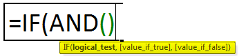
The IF AND formula can be applied as follows:
“=IF(AND (Condition 1,Condition 2,…),Value _if _True,Value _if _False)”
You are free to use this image on your website, templates, etc, Please provide us with an attribution linkArticle Link to be Hyperlinked
For eg:
Source: IF AND in Excel (wallstreetmojo.com)
How to Use IF AND Excel Statement?
You can download this IF AND Formula Excel Template here – IF AND Formula Excel Template
Let us understand the usage of the IF AND formula with the help of some examples mentioned below:
Example #1
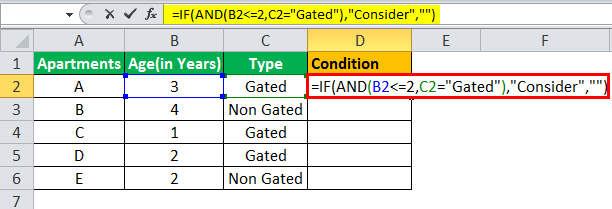
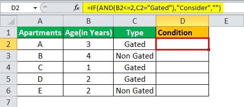
The table given below provides a list of apartments along with their age (in years) and type of society. Now we need to perform a comparative analysis for the apartments based on the age of the building and the type of society.
Here, we use the combination of less than equal (<=) to operator and the equal to (=) text functions in the condition to be demonstrated for IF AND function.
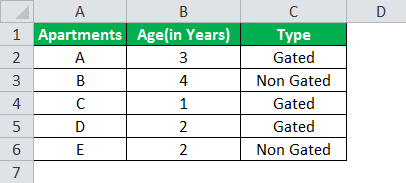
- The IF AND formula used to perform the analysis is stated as follows:
“=IF(AND(B2<=2,C2=“Gated”),“Consider”, “”)”
- The succeeding image shows the IF AND condition applied to perform the evaluation.
- Press “Enter” to get the answer.
- Drag the formula to find the results for all the apartments.
The results in the cell D of the above table shows that the IF AND formula will be performing one among the following:
- If both the arguments entered in the AND function is “true,” then the IF function will return that apartment to be “Consider.”
- If either of the arguments in the AND functionThe AND function in Excel is classified as a logical function; it returns TRUE if the specified conditions are met, otherwise it returns FALSE.read more is “false” or both the arguments entered are “false,” then the IF function will return a blank string.
The IF AND formula can also perform calculations based on whether the AND function returns “true” or “false,” apart from returning only the predefined text strings.
We will understand this concept with the help of the below-mentioned example.
Example #2
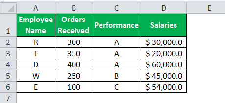
The given data tableA data table in excel is a type of what-if analysis tool that allows you to compare variables and see how they impact the result and overall data. It can be found under the data tab in the what-if analysis section.read more has the list of employee name along with their orders received, performance, and salaries. Calculate the employee hike (or bonus) based on two parameters–the number of orders received and performance.
The criteria to calculate the bonus is as follows.
- The number of orders received is greater than or equal to 200, and the performance is equal to “A.”
- The IF AND formula will be,
“=IF(AND(B2>=200,C2= “A”),D2*10%,D2*5%)”
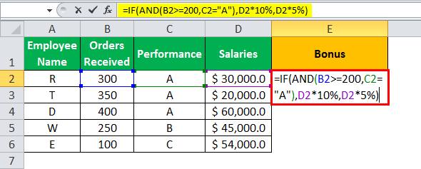
- Press “Enter” to get the final output. The bonus appears in cell E2.
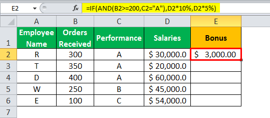
- Drag the formula to find the bonus of all employees.
Based on these results, the IF formula does the following evaluation:
- If both the conditions are satisfied, the AND function returns “true,” then the bonus received is calculated as salary multiplied by 10%.
- If either one or both the conditions are found to be “false” by the AND function, then the bonus is calculated as salary multiplied by 5%.
Examples 1 and 2 have only two criteria to test and evaluate. Using multiple arguments or conditions to test them for “true” or “false” is also allowed.
Example #3
Let us evaluate multiple criteria and use AND function.
A table with five stocks and their parameter details including financial ratiosFinancial ratios are indications of a company’s financial performance. There are several forms of financial ratios that indicate the company’s results, financial risks, and operational efficiency, such as the liquidity ratio, asset turnover ratio, operating profitability ratios, business risk ratios, financial risk ratio, stability ratios, and so on.read more, such as ROCEReturn on Capital Employed (ROCE) is a metric that analyses how effectively a company uses its capital and, as a result, indicates long-term profitability. ROCE=EBIT/Capital Employed.read more, ROEReturn on Equity (ROE) represents financial performance of a company. It is calculated as the net income divided by the shareholders equity. ROE signifies the efficiency in which the company is using assets to make profit.read more, Debt to equityThe debt to equity ratio is a representation of the company’s capital structure that determines the proportion of external liabilities to the shareholders’ equity. It helps the investors determine the organization’s leverage position and risk level. read more, and PE ratioThe price to earnings (PE) ratio measures the relative value of the corporate stocks, i.e., whether it is undervalued or overvalued. It is calculated as the proportion of the current price per share to the earnings per share. read more is provided (shown in the below table). Using this data lets us test the condition to invest in suitable stocks. That is, using the parameters, let us analyze the stocks to derive the best investment horizonThe term «investment horizon» refers to the amount of time an investor is expected to hold an investment portfolio or a security before selling it. Depending on the need for funds and risk appetite, the investor may invest for a few days or hours to a few years or decades.read more, which is important for growth.
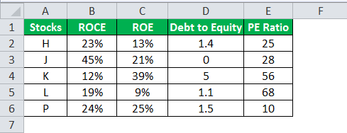
The following syntax is used where the conditions are applied to arrive at the result (shown in the below table).
“=IF(AND(B2>18%,C2>20%,D2<2,E2<30%),“Invest”,“”)”

- Press “Enter” to get the final output (Investment Criteria) of the above formula.

- Drag the formula to find the Investment Criteria.
In the above data table, the AND function tests for the parameters using the operators. The resulting output generated by the IF formula is as follows:
- If all the four criteria mentioned in the AND function are tested and satisfied, then the IF function returns the “Invest” text string.
- If either one or more among the four conditions or all the four conditions fail to satisfy the AND function, then the IF function returns empty strings (“”).
The Characteristics of IF AND function
- The IF AND function does not differentiate between case-insensitive texts.
- The AND function can be used to evaluate up to 255 conditions for “true” or “false,” and the total formula length does not exceed 8192 characters.
- Text values or blank cells are given as an argument to test the conditions in AND function.
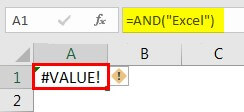
- The AND formula will return “#VALUE!” if there is no logical output found while evaluating the conditions.
- IF AND excel statement is a combination of two logical functions that tests and evaluates multiple conditions.
- The output of the AND function is based on, whether the IF function will return the value “true” or “false,” respectively.
- IF function is used to test a single criterion whereas, the AND function is used to test multiple criteria.
- The syntax of the IF AND formula is:
“=IF(AND (Condition 1,Condition 2,…),Value _if _True,Value _if _False)”
- The IF AND formula also performs a calculation based on whether the AND function is “true” or “false” apart from returning only the predefined text strings.
Frequently Asked Questions
1. How to use IF AND function in Excel?
The IF AND excel statement is the two logical functions often nested together.
Syntax:
“=IF(AND(Condition1,Condition2, value_if_true,vaue_if_false)”
The IF formula is used to test and compare the conditions expressed, along with the expected value. It provides the desired result if the condition is either “true” or “false.”
The AND formula is used to test multiple criteria. It returns “true” if all the given conditions are satisfied, or else returns “false.”
2. What is the IF AND function in Excel?
IF AND formula is applied as the combination of the two logical functions that enable the user to evaluate the multiple conditions. Based on the output of the AND function, the IF function returns the output “true” or “false.”
3. How to combine IF and AND functions in Excel?
To combine IF and AND functions, you need to replace the “condition_test” argument in the IF function with AND function.
“=IF(condition_test, value_if_true,vaue_if_false)”
“=IF(AND(Condition1,Condition2, value_if_true,vaue_if_false)”
In AND function we can use multiple conditions.
Recommended Articles
This has been a guide to IF AND function in Excel. Here we discuss how to use IF Formula combined with AND function along with examples and downloadable templates. You may also look at these useful functions in Excel –
- IF EXCEL FunctionIF function in Excel evaluates whether a given condition is met and returns a value depending on whether the result is “true” or “false”. It is a conditional function of Excel, which returns the result based on the fulfillment or non-fulfillment of the given criteria.
read more - Average IF Function
- SUMIF with Multiple CriteriaThe SUMIF (SUM+IF) with multiple criteria sums the cell values based on the conditions provided. The criteria are based on dates, numbers, and text. The SUMIF function works with a single criterion, while the SUMIFS function works with multiple criteria in excel.read more
- Nested If ConditionIn Excel, nested if function means using another logical or conditional function with the if function to test multiple conditions. For example, if there are two conditions to be tested, we can use the logical functions AND or OR depending on the situation, or we can use the other conditional functions to test even more ifs inside a single if.read more
Логический оператор ЕСЛИ в Excel применяется для записи определенных условий. Сопоставляются числа и/или текст, функции, формулы и т.д. Когда значения отвечают заданным параметрам, то появляется одна запись. Не отвечают – другая.
Логические функции – это очень простой и эффективный инструмент, который часто применяется в практике. Рассмотрим подробно на примерах.
Синтаксис функции ЕСЛИ с одним условием
Синтаксис оператора в Excel – строение функции, необходимые для ее работы данные.
=ЕСЛИ (логическое_выражение;значение_если_истина;значение_если_ложь)
Разберем синтаксис функции:
Логическое_выражение – ЧТО оператор проверяет (текстовые либо числовые данные ячейки).
Значение_если_истина – ЧТО появится в ячейке, когда текст или число отвечают заданному условию (правдивы).
Значение,если_ложь – ЧТО появится в графе, когда текст или число НЕ отвечают заданному условию (лживы).
Пример:
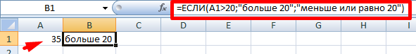
Оператор проверяет ячейку А1 и сравнивает ее с 20. Это «логическое_выражение». Когда содержимое графы больше 20, появляется истинная надпись «больше 20». Нет – «меньше или равно 20».
Внимание! Слова в формуле необходимо брать в кавычки. Чтобы Excel понял, что нужно выводить текстовые значения.
Еще один пример. Чтобы получить допуск к экзамену, студенты группы должны успешно сдать зачет. Результаты занесем в таблицу с графами: список студентов, зачет, экзамен.
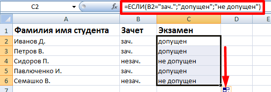
Обратите внимание: оператор ЕСЛИ должен проверить не цифровой тип данных, а текстовый. Поэтому мы прописали в формуле В2= «зач.». В кавычки берем, чтобы программа правильно распознала текст.
Функция ЕСЛИ в Excel с несколькими условиями
Часто на практике одного условия для логической функции мало. Когда нужно учесть несколько вариантов принятия решений, выкладываем операторы ЕСЛИ друг в друга. Таким образом, у нас получиться несколько функций ЕСЛИ в Excel.
Синтаксис будет выглядеть следующим образом:
=ЕСЛИ(логическое_выражение;значение_если_истина;ЕСЛИ(логическое_выражение;значение_если_истина;значение_если_ложь))
Здесь оператор проверяет два параметра. Если первое условие истинно, то формула возвращает первый аргумент – истину. Ложно – оператор проверяет второе условие.
Примеры несколько условий функции ЕСЛИ в Excel:
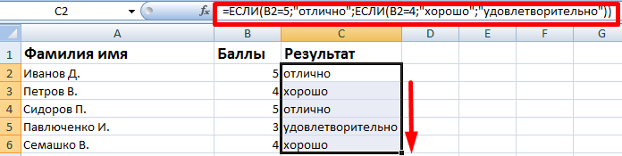
Таблица для анализа успеваемости. Ученик получил 5 баллов – «отлично». 4 – «хорошо». 3 – «удовлетворительно». Оператор ЕСЛИ проверяет 2 условия: равенство значения в ячейке 5 и 4.
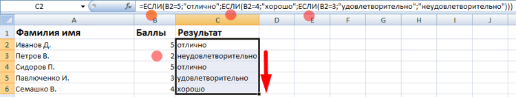
В этом примере мы добавили третье условие, подразумевающее наличие в табеле успеваемости еще и «двоек». Принцип «срабатывания» оператора ЕСЛИ тот же.
Расширение функционала с помощью операторов «И» и «ИЛИ»
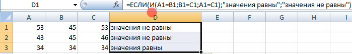
Когда нужно проверить несколько истинных условий, используется функция И. Суть такова: ЕСЛИ а = 1 И а = 2 ТОГДА значение в ИНАЧЕ значение с.
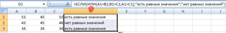
Функция ИЛИ проверяет условие 1 или условие 2. Как только хотя бы одно условие истинно, то результат будет истинным. Суть такова: ЕСЛИ а = 1 ИЛИ а = 2 ТОГДА значение в ИНАЧЕ значение с.
Функции И и ИЛИ могут проверить до 30 условий.
Пример использования оператора И:
Пример использования функции ИЛИ:
Как сравнить данные в двух таблицах
Пользователям часто приходится сравнить две таблицы в Excel на совпадения. Примеры из «жизни»: сопоставить цены на товар в разные привозы, сравнить балансы (бухгалтерские отчеты) за несколько месяцев, успеваемость учеников (студентов) разных классов, в разные четверти и т.д.
Чтобы сравнить 2 таблицы в Excel, можно воспользоваться оператором СЧЕТЕСЛИ. Рассмотрим порядок применения функции.
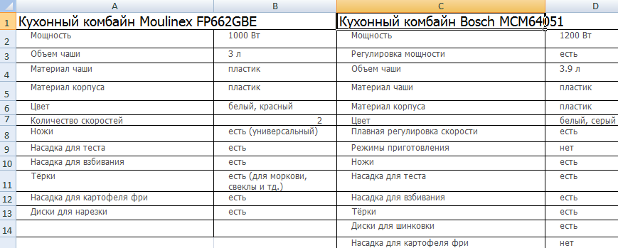
Для примера возьмем две таблицы с техническими характеристиками разных кухонных комбайнов. Мы задумали выделение отличий цветом. Эту задачу в Excel решает условное форматирование.
Исходные данные (таблицы, с которыми будем работать):
Выделяем первую таблицу. Условное форматирование – создать правило – использовать формулу для определения форматируемых ячеек:
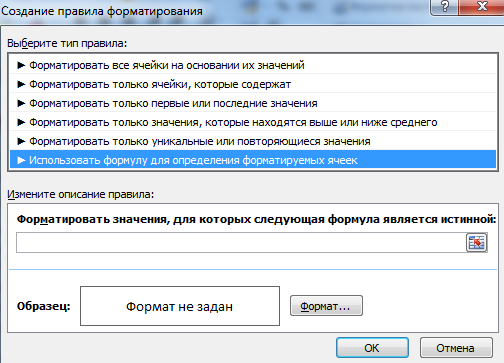
В строку формул записываем: =СЧЕТЕСЛИ (сравниваемый диапазон; первая ячейка первой таблицы)=0. Сравниваемый диапазон – это вторая таблица.
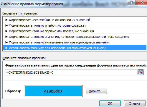
Чтобы вбить в формулу диапазон, просто выделяем его первую ячейку и последнюю. «= 0» означает команду поиска точных (а не приблизительных) значений.
Выбираем формат и устанавливаем, как изменятся ячейки при соблюдении формулы. Лучше сделать заливку цветом.
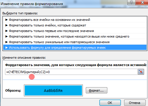
Выделяем вторую таблицу. Условное форматирование – создать правило – использовать формулу. Применяем тот же оператор (СЧЕТЕСЛИ).
Скачать все примеры функции ЕСЛИ в Excel
Здесь вместо первой и последней ячейки диапазона мы вставили имя столбца, которое присвоили ему заранее. Можно заполнять формулу любым из способов. Но с именем проще.
What is the IF AND Function in Excel?
IF AND function in Excel is a powerful combination of logical functions in Excel that allows users to evaluate multiple conditions in a single formula. It simplifies calculations by returning “TRUE” or “FALSE” results based on whether all specified conditions are met, making data analysis more efficient and accurate.
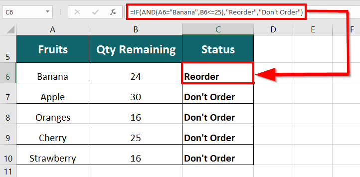
For example, =IF(AND(A6=”Banana”,B6<=25),”Reorder”,”Don’t Order”) can help decide whether to reorder bananas.
If both conditions are true, the function will return “Reorder” to indicate the need for more bananas; otherwise, it will return “Don’t Order” to signify no need for reordering.
We can automate processes, reduce errors, and make informed decisions based on data by using IF AND statements. They are particularly useful in determining whether an employee qualifies for a promotion or incentive, verifying a customer’s eligibility for a discount, or checking the delivery status of customer orders.
Key Highlights
- The IF function’s output depends on whether the AND function returns TRUE or FALSE.
- We can nest the IF AND function within other Excel functions for complex tests.
- Other logical functions like OR or NOT can replace the AND function based on specific conditions.
Syntax of IF AND Function in Excel
IF(AND(Logical1, Logical2,…), val_if_true, val_if_false)
Explanation:
- Logical1, Logical2: Test/ compare values of specified cells
- Value_if_true: Value Excel returns if the condition is satisfied
- Value_if_false: Value Excel returns if the condition is not satisfied
How to Use the IF AND Function in Excel?
You can download this IF AND Function Excel Template here – IF AND Function Excel Template
#1 Testing Two Conditions
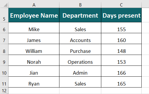
A] Consider the table below consisting of Employee Names, Departments, and the days they were present in six months. Employees are eligible for the promotion if they belong to the Sales department and are present for at least 160 days. We will use the IF AND function in Excel to check the two conditions.
To use the function, follow these steps:
Step 1: Create a new column heading called “Eligible for Promotion.”
Step 2: Select the cell where you want to display the result (let’s assume it is cell D6), and type the formula =IF(AND(B6=”Sales”,C6>=160),”Yes”,”No”).
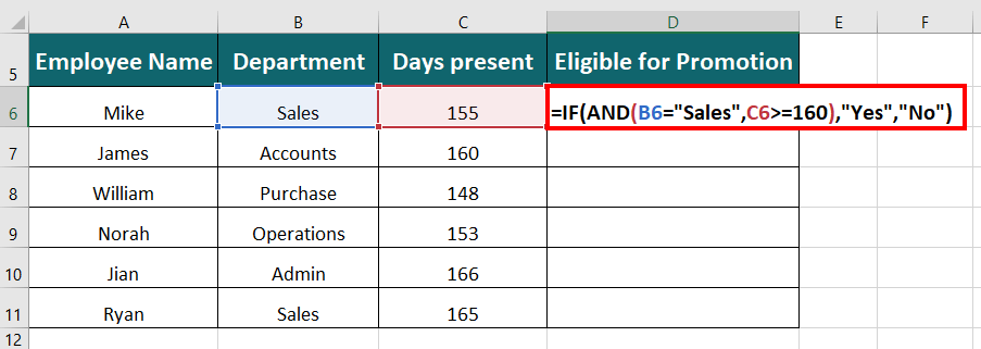
Here’s how the formula works:
1. The AND function checks two conditions:
- Condition 1 (B6=”Sales”): If an employee belongs to the Sales department.
- Condition 2 (C6>=160): If the employee was present for at least 160 days.
2. If the values meet both conditions, the AND function returns TRUE and passes this information to the IF function.
3. The IF function then returns the value “Yes” if the condition is TRUE and “No” if it’s FALSE.
Step 2: Press Enter key to see the result
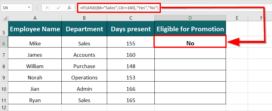
Result- Employee Mike belongs to the Sales department but was present for less than 160 days. As he satisfies only one condition, he is not eligible for the promotion.
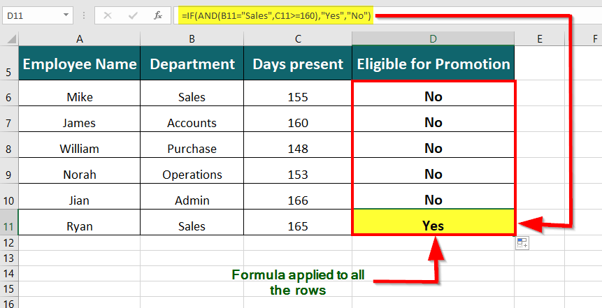
Step 3: To check the eligibility of remaining employees, drag the formula into the other cells
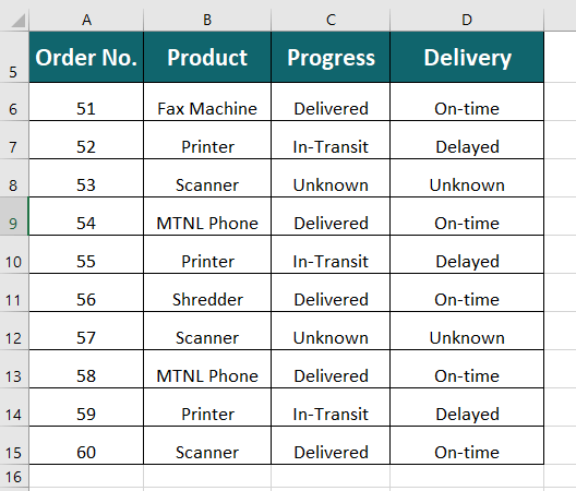
B] Below is a table that shows a list of orders along with their respective products, Progress, and Delivery status. We aim to determine whether the final order status has been closed or is still open.
Follow these steps to understand how to check the final order status:
Step 1: Create a new column called “Status.”
Step 2: In an empty cell, such as E6, enter the formula =IF(AND(C6=”Delivered”,D6=”On-time”),”Closed”,”Open”).
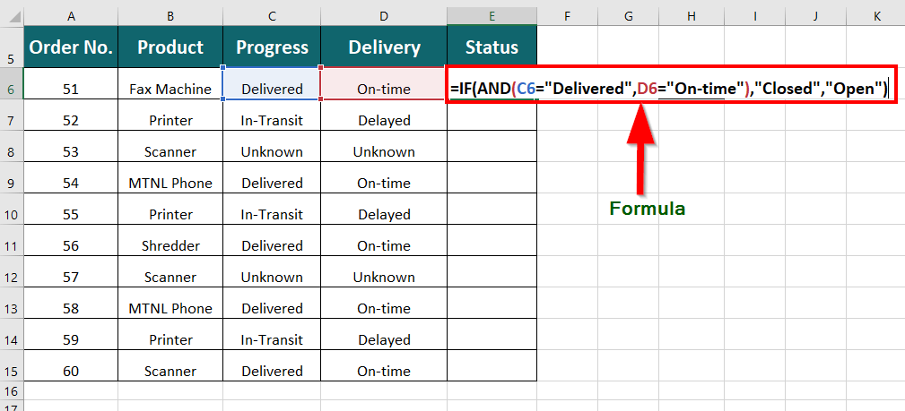
Explanation of the formula:
1. The AND function verifies two conditions:
-
- Condition 1 (C6=”Delivered”): It checks if an order’s Progress is marked as “Delivered.”
- Condition 2 (D6=”On-time”): It verifies if the order was delivered “On-time.”
2. When both conditions satisfy, the AND function returns a TRUE value, which is passed to the IF function.
3. The IF function then returns “Closed” if the condition is TRUE and “Open” if it’s FALSE.
Step 3: Press Enter key to get the result
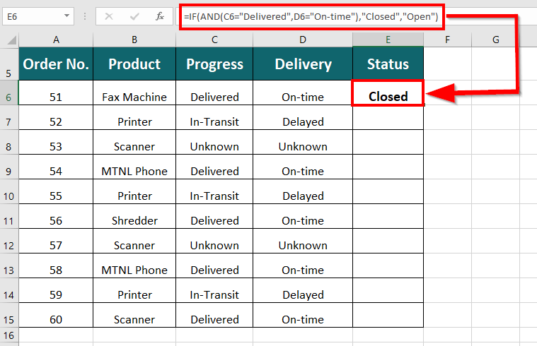
Result- The Progress status for Order No. 51 is Delivered, and it was delivered on time, i.e., it satisfies both conditions. Therefore, the IF AND formula returns “Closed” for that order.
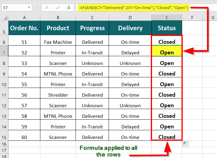
Step 4: Drag the formula into the remaining cells to check the remaining orders’ current status.
#2 Nested IF AND Statement
A Nested IF AND Statement in Excel is like a set of nested (embedded) boxes where each box has an IF AND condition to test. Here’s an example of a nested IF AND statement.
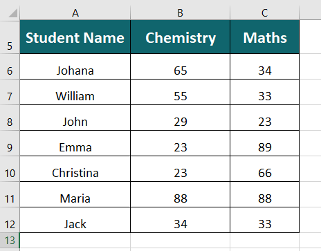
We have a list of students with their marks in Chemistry and Maths, and we want to evaluate their performance based on their marks in the two subjects.
Here’s how we can use the IF AND Function in Excel to check the student’s performance-
Step 1: Create a new column heading “Performance”.
Step 2: In an empty cell (e.g., D6), enter the formula:
=IF(AND(B6<30,C6<25),”Poor”,IF(AND(B6>60,C6>30),”Excellent”,”Average”))
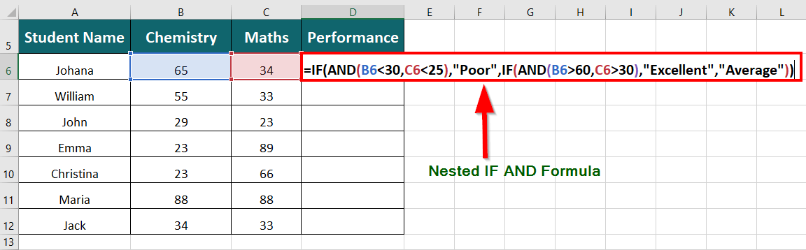
Note: It is known as a Nested IF AND statement because one IF AND formula appears inside the other. In other words, two IF AND statements are in a single formula.
Explanation of the Formula:
1. The first AND formula check two conditions:
- Condition 1 (B6<30): If marks scored in Chemistry are less than 30
- Condition 2 (C6<25): If marks scored in Maths are less than 25.
If both conditions satisfy, the AND function returns TRUE and passes the information to the first IF function, which displays the result as Poor.
2. The second AND formula check two conditions:
- Condition 1 (B6>60): If marks scored in Chemistry is more than 60.
- Condition 2 (C6>30)): If marks scored in Maths is more than 30.
If both conditions are satisfied, the AND function returns TRUE and passes the information to the second IF function, which displays the result as Excellent. If not, the formula shows the result as Average.
Step 3: Press Enter key to get the output
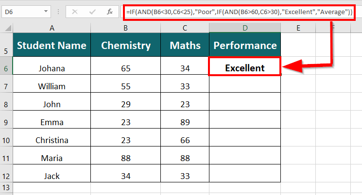
Result- Johana has scored more than 60 marks in Chemistry and more than 30 marks in Maths, satisfying both conditions. As a result, the Nested IF AND formula display the output as Excellent
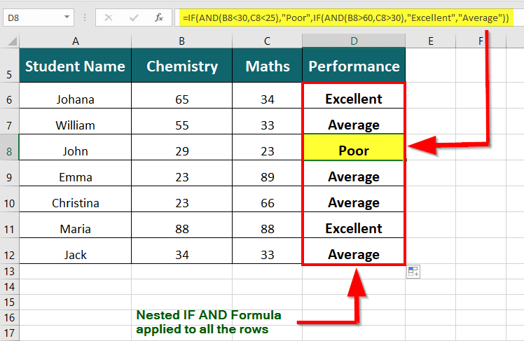
Step 4: Drag the Nested IF AND formula into the remaining cells to get the performance of the remaining students.
#3 Alternatives to the IF AND Function
There are two logical functions to use instead of AND, depending on the specific situation: OR and NOT.
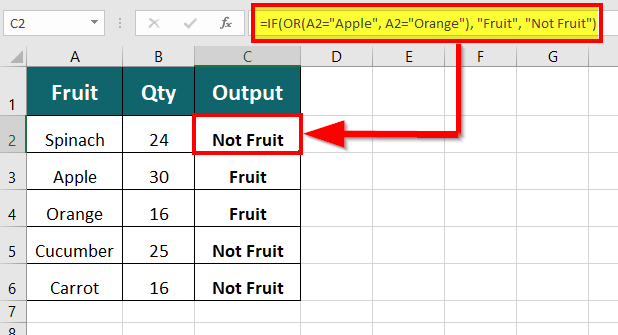
1. OR Function
It is to test whether at least one of several conditions is true.
For instance, the formula =IF(OR(A2=”Apple”, A2=”Orange”), “Fruit”, “Not Fruit”) will display “Fruit” if cell A2 contains either “Apple” or “Orange,” and “Not Fruit” if it has any other value.
2. NOT Function
It returns the opposite of the result of another logical function.
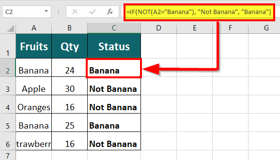
For example, the formula =IF(NOT(A2=”Banana”), “Not Banana”, “Banana”) will return “Not Banana” if cell A2 does not contain “Banana” and “Banana” otherwise.
It is crucial to choose the most appropriate function based on the conditions being tested. Additionally, these functions can be nested to create more complex formulas.
Things To Remember
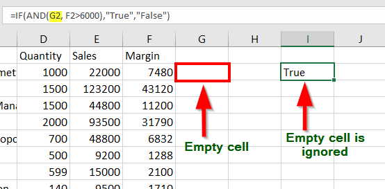
- If any argument is an empty cell, the IF AND function ignore it. However, if all arguments are empty cells, Excel returns a #VALUE! Error.
- In newer versions of Excel, including Excel 2007 and later versions, you can include up to 255 arguments in the formula of the IF AND function. For previous versions of Excel, Microsoft had limited the AND function to test a maximum of 30 conditions at a time.
- You can use a combination of text and numeric values, cell references, boolean values, and comparison operators as arguments in the IF AND function. But it can’t handle strings. If the arguments are characters, then AND returns a #VALUE! error.
Best Practices
- Use descriptive cell and range names instead of cell references to simplify formulas. For instance, consider the formula: =IF(AND(MathGrade>=70,ScienceGrade>=60),”Pass”,”Fail”)
In this formula, “MathGrade” and “ScienceGrade” are named ranges that refer to the appropriate columns in the table.
- Avoid common mistakes when using the IF AND function, such as forgetting to close all parentheses or improperly nesting the functions.
- Thoroughly test the formula by inputting different values and conditions to ensure it returns expected outcomes in all scenarios before using it in more extensive spreadsheets or analyses.
Frequently Asked Questions (FAQs)
Q1. How do you use IF and AND in Excel together?
Answer: To use the IF and AND functions together in Excel, you can create a formula like this:
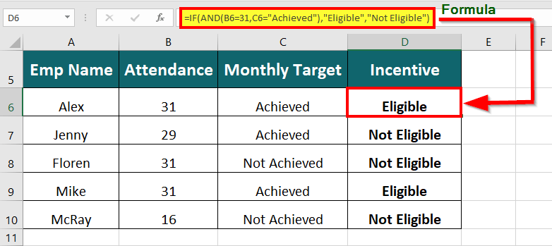
=IF(AND(B6=31,C6=”Achieved”),”Eligible”,”Not Eligible”)
In this example, we are checking whether an employee is eligible for an incentive based on two criteria: attendance and achieving a monthly target.
- The AND function checks whether the employee was present for 31 days a month (using cell B6) and whether they achieved their monthly target (using cell C6).
- If the cell values meet both criteria, the AND function returns TRUE, and the IF function displays “Eligible” as a result.
- If the cell values meet either criterion, the AND function returns FALSE, and the IF function displays “Not Eligible” as a result.
Q2. Can you have 2 IF AND statements in Excel?
Answer: Yes, you can use two IF AND statements in a single formula in excel to check multiple criteria. For instance, consider the formula
=IF(AND(B6>=25000,C6=”Digital Wallet”),”20% “,IF(AND(B6>=20000,C6=”Credit Card”),”10%”,”No Discount”))
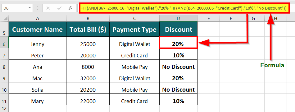
In this formula:
- The first IF AND statement check whether a customer has a purchase total greater than or equal to $25,000 and whether the customer chooses to pay through a digital wallet.
If both conditions are met, the formula returns a 20% discount on the total bill.
- The second IF AND statement check whether a customer has a purchase total greater than or equal to $20,000 and whether the customer chooses to pay through a credit card.
If both conditions are met, the formula returns a 10% discount on the total bill. If neither of these conditions is met, the formula returns “No Discount“.
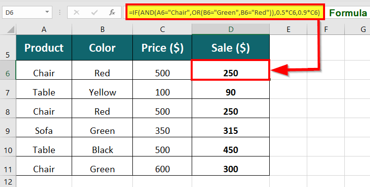
Q3. Can you use IF AND and OR together in Excel?
Answer: Yes, you can use IF AND and OR functions together in Excel to evaluate multiple criteria in a single formula. For example, consider the formula:
=IF(AND(A6=”Chair”,OR(B6=”Green”,B6=”Red”)),0.5*C6,0.9*C6)
In this formula, the AND function checks if the product is a chair and if its color is either green or red. If the AND function is TRUE, the IF formula reduces the product price by 50%, and if it is FALSE, it reduces the price by 10%.
Recommended Article
The above article is a guide to using the IF AND Function in Excel, along with examples and downloadable templates. For more comprehensive articles, EDUCBA recommends the following articles-
- Excel Basic Functions
- HLOOKUP in Excel
- Excel Count Function
- Excel INDEX Function
- Если и функция в Excel
Функция Excel IF и AND (Содержание)
- Если и функция в Excel
- Как использовать функцию IF и в Excel?
Если и функция в Excel
Цель этого руководства — показать, как объединить функции IF и AND в Excel, чтобы проверить несколько условий в одной формуле. Некоторые предметы в природе конечны. Другие, кажется, обладают бесконечным потенциалом, и, что интересно, функция IF, похоже, обладает такими свойствами.
Наша цель сегодня — увидеть, как и если мы можем объединить IF и функцию AND для одновременной оценки нескольких условий. Итак, во-первых, нам нужно будет построить функцию IF AND, и для этого нам потребуется объединить две отдельные функции — функции IF и AND в одну формулу. Давайте посмотрим, как этого можно достичь:
ЕСЛИ (И (логическое1, логическое2, …), val_if_true, val_if_false)

Приведенная выше формула имеет следующее значение: если первое условие, то есть условие 1, истинно, а второе условие, то есть условие 2, также истинно, то сделайте что-нибудь или сделайте что-то другое.
Как использовать функцию IF и в Excel?
Давайте разберемся, как использовать функцию IF AND в Excel, используя несколько примеров.
Вы можете скачать этот шаблон Excel с функцией IF AND Function здесь.
Функция Excel IF и AND — Пример № 1
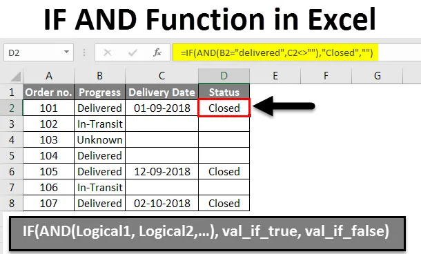
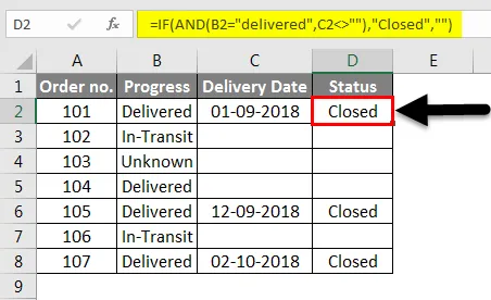
Давайте разберемся в этом на примере, создадим формулу, цель которой — проверить, доставлен ли B2, а также убедиться, что C2 не пуст. Теперь, в зависимости от результата, будет выполнено одно из следующих действий:
- Если и условие 1, и условие 2 оцениваются как ИСТИНА, то заказ должен быть помечен как «Закрыто».
- Если какое-либо из условий оценивается как FALSE или оба оценивают как FALSE, то должна быть возвращена пустая строка («»).
= ЕСЛИ (И (В2 = «доставлено», C2 »»), «Закрыто», «»)
Функция ЕСЛИ И показана на скриншоте ниже:
Примечание. При использовании формулы IF AND для оценки определенных условий важно помнить, что прописные и строчные буквы считаются одинаковыми. Итак, если целью является использование чувствительной к регистру версии формулы IF AND, мы должны заключить аргументы AND в функцию EXACT.
Функция Excel IF и AND — Пример № 2
До сих пор в нашем предыдущем примере мы пытались проверить два состояния разных ячеек. Но в повседневной жизни мы часто сталкиваемся с ситуациями, когда нам может потребоваться выполнить несколько тестов в одной ячейке. Примером, который обычно демонстрирует это, является проверка, находится ли значение ячейки между двумя числами. Вот где функция IF И пригодится!
Теперь давайте предположим, что у нас есть номера продаж для определенных заказов в столбце B, и наша задача — пометить суммы, которые меньше, чем 100 долларов США, но больше, чем 50 долларов США. Итак, чтобы решить эту проблему, сначала мы вставим следующую формулу в ячейку C2, а затем перейдем к ее копированию по столбцам:
= ЕСЛИ (И (В2> 50, В2 <100), «Х», «»)

Функция Excel IF и AND — Пример № 3
Если требуется, чтобы мы включили периферийные значения (100 и 50), то нам нужно будет использовать оператор больше или равно (> =) и оператор меньше или равно (<=):
= IF (AND (B2> = 50, B2 <= 100), «X», «»)

Теперь, чтобы обработать другие виды периферийных значений без изменения формулы, мы введем максимальное и минимальное числа в двух разных ячейках и предоставим ссылку на эти ячейки в нашей формуле. Чтобы формула функционировала надлежащим образом для всех строк, обязательно используйте абсолютные ссылки для периферийных ячеек (в данном случае $ F $ 1 и $ F $ 2):
Теперь мы будем применять формулу в ячейке C2.
= IF (AND (B2> = $ F $ 1, B2 <= $ F $ 2), «X», «»)

Функция Excel IF и AND — Пример № 4
Используя формулу, аналогичную приведенной выше, можно проверить, находится ли дата в определенном диапазоне .
Например, мы будем отмечать все даты между 30 сентября 2018 года и 10 сентября 2018 года, включая периферийные даты. Итак, здесь мы видим, что мы столкнулись с уникальной проблемой, заключающейся в том, что даты не могут быть напрямую предоставлены для логических тестов. Чтобы сделать даты понятными для Excel, нам нужно будет заключить их в функцию DATEVALUE, как показано ниже:
= IF (AND (B2> = DATEVALUE («10-Sep-2018»), B2 <= DATEVALUE («30-Sep-2018»)), «X», «»)

Также можно просто ввести даты «Кому» и «От» в ячейки (в нашем примере $ F $ 2 и $ F $ 1), а затем извлечь их из исходных ячеек, используя формулу IF AND:
= IF (AND (B2> = $ F $ 1, B2 <= $ F $ 2), «X», «»)

Функция Excel IF и AND — Пример № 5
Помимо возврата предопределенных значений, функция IF И также может выполнять различные вычисления, основанные на том, являются ли упомянутые условия ЛОЖНЫМИ или ИСТИНАМИ.
У нас есть список студентов и их результаты тестов в процентах. Теперь нам нужно оценить их. Таблица процента к оценке приведена ниже.

Как видно из приведенной выше таблицы, если процент выше 90%, то соответствующая оценка для этой оценки — A +. Если набранный процент составляет от 85% до 90%, тогда оценка составляет A. Если процент составляет от 80% до 85%, тогда оценка составляет B +. Если процент составляет от 75% до 80%, тогда оценка составляет B. Если процент составляет от 70% до 75%, тогда оценка составляет C +. Если процент составляет от 60% до 70%, тогда оценка составляет C. Если процент составляет от 50% до 60%, тогда оценка составляет D +. Если процент составляет от 40% до 50%, тогда оценка равна D. И, наконец, если процент ниже 40%, тогда оценка равна F.
Теперь список студентов и их процент показан ниже:

Формула, которую мы будем использовать:
= ЕСЛИ (С2>»90″%»А +», ЕСЛИ (И (С2>»85″%, С2 =»80″%, С2 =»75″%, С2 =»70″%, С2 =»60 «%, С2 =» 50 «%, С2 =» 40 «%, С2 <=» 50 «%), » D», » F»))))))))
Мы использовали Nested IF, а также использовали несколько AND вместе с ними.
Функция IF оценивает условие, предоставленное в своем аргументе и на основе результата (ИСТИНА или ЛОЖЬ), возвращает один вывод или другой.
Формула IF выглядит следующим образом:

Здесь Logical_Test — это условие, которое будет оценено. В зависимости от результата будет возвращено либо Value_If_True, либо Value_If_False.
В первом случае, т. Е. Для Student1, мы видим, что процент составляет 74%, таким образом, результат возвращается в соответствии с таблицей процентного соотношения к классу, показанной выше.

Точно так же для Студента 2 мы видим, что процент составляет 76%, таким образом, результат, возвращаемый согласно таблице процентного соотношения к классу, показанной выше, будет B, так как процент между> 75% и 80% получает оценку B.
Перетаскивая формулу, примененную в ячейке D2, другие учащиеся также получают аналогичные оценки.

Что нужно помнить об IF и функции в Excel
- Функция IF AND имеет предел и может проверять до 255 условий. Это, конечно, применимо только к Excel 2007 и выше. Для предыдущих версий Excel функция AND была ограничена только 30 условиями.
- Функция IF AND может обрабатывать логические аргументы и работает даже с числами. Но он не может обрабатывать строки. Если предоставленные аргументы являются символами, тогда AND возвращает # ЗНАЧЕНИЕ! ошибка.


- При работе с большими наборами данных высока вероятность того, что нам может потребоваться проверить несколько разных наборов различных условий AND одновременно. В такие моменты нам нужно использовать вложенную форму формулы IF AND:
ЕСЛИ (И (…), выход1 , ЕСЛИ (И (…), выход2 , ЕСЛИ (И (…), выход 3 , ЕСЛИ (И (…) выход4 )))

Рекомендуемые статьи
Это руководство по IF и функции в Excel. Здесь мы обсудим, как использовать функцию IF AND в Excel вместе с практическими примерами и загружаемым шаблоном Excel. Вы также можете просмотреть наши другие предлагаемые статьи —
- Многократная функция IFS в Excel
- Как использовать функцию И в Excel?
- Как использовать функцию COUNTIF Excel?
- Руководство по COUNTIF с несколькими критериями
Things will not always be the way we want them to be. The unexpected can happen. For example, let’s say you have to divide numbers. Trying to divide any number by zero (0) gives an error. Logical functions come in handy such cases. In this tutorial, we are going to cover the following topics.
In this tutorial, we are going to cover the following topics.
- What is a Logical Function?
- IF function example
- Excel Logic functions explained
- Nested IF functions
What is a Logical Function?
It is a feature that allows us to introduce decision-making when executing formulas and functions. Functions are used to;
- Check if a condition is true or false
- Combine multiple conditions together
What is a condition and why does it matter?
A condition is an expression that either evaluates to true or false. The expression could be a function that determines if the value entered in a cell is of numeric or text data type, if a value is greater than, equal to or less than a specified value, etc.
IF Function example
We will work with the home supplies budget from this tutorial. We will use the IF function to determine if an item is expensive or not. We will assume that items with a value greater than 6,000 are expensive. Those that are less than 6,000 are less expensive. The following image shows us the dataset that we will work with.
 and conditions in Excel")
- Put the cursor focus in cell F4
- Enter the following formula that uses the IF function
=IF(E4<6000,”Yes”,”No”)
HERE,
- “=IF(…)” calls the IF functions
- “E4<6000” is the condition that the IF function evaluates. It checks the value of cell address E4 (subtotal) is less than 6,000
- “Yes” this is the value that the function will display if the value of E4 is less than 6,000
-
“No” this is the value that the function will display if the value of E4 is greater than 6,000
When you are done press the enter key
You will get the following results
 and conditions in Excel")
Excel Logic functions explained
The following table shows all of the logical functions in Excel
| S/N | FUNCTION | CATEGORY | DESCRIPTION | USAGE |
|---|---|---|---|---|
| 01 | AND | Logical | Checks multiple conditions and returns true if they all the conditions evaluate to true. | =AND(1 > 0,ISNUMBER(1)) The above function returns TRUE because both Condition is True. |
| 02 | FALSE | Logical | Returns the logical value FALSE. It is used to compare the results of a condition or function that either returns true or false | FALSE() |
| 03 | IF | Logical |
Verifies whether a condition is met or not. If the condition is met, it returns true. If the condition is not met, it returns false. =IF(logical_test,[value_if_true],[value_if_false]) |
=IF(ISNUMBER(22),”Yes”, “No”) 22 is Number so that it return Yes. |
| 04 | IFERROR | Logical | Returns the expression value if no error occurs. If an error occurs, it returns the error value | =IFERROR(5/0,”Divide by zero error”) |
| 05 | IFNA | Logical | Returns value if #N/A error does not occur. If #N/A error occurs, it returns NA value. #N/A error means a value if not available to a formula or function. |
=IFNA(D6*E6,0) N.B the above formula returns zero if both or either D6 or E6 is/are empty |
| 06 | NOT | Logical | Returns true if the condition is false and returns false if condition is true |
=NOT(ISTEXT(0)) N.B. the above function returns true. This is because ISTEXT(0) returns false and NOT function converts false to TRUE |
| 07 | OR | Logical | Used when evaluating multiple conditions. Returns true if any or all of the conditions are true. Returns false if all of the conditions are false |
=OR(D8=”admin”,E8=”cashier”) N.B. the above function returns true if either or both D8 and E8 admin or cashier |
| 08 | TRUE | Logical | Returns the logical value TRUE. It is used to compare the results of a condition or function that either returns true or false | TRUE() |
A nested IF function is an IF function within another IF function. Nested if statements come in handy when we have to work with more than two conditions. Let’s say we want to develop a simple program that checks the day of the week. If the day is Saturday we want to display “party well”, if it’s Sunday we want to display “time to rest”, and if it’s any day from Monday to Friday we want to display, remember to complete your to do list.
A nested if function can help us to implement the above example. The following flowchart shows how the nested IF function will be implemented.
 and conditions in Excel")
The formula for the above flowchart is as follows
=IF(B1=”Sunday”,”time to rest”,IF(B1=”Saturday”,”party well”,”to do list”))
HERE,
- “=IF(….)” is the main if function
- “=IF(…,IF(….))” the second IF function is the nested one. It provides further evaluation if the main IF function returned false.
Practical example
 and conditions in Excel")
Create a new workbook and enter the data as shown below
 and conditions in Excel")
- Enter the following formula
=IF(B1=”Sunday”,”time to rest”,IF(B1=”Saturday”,”party well”,”to do list”))
- Enter Saturday in cell address B1
- You will get the following results
 and conditions in Excel")
Download the Excel file used in Tutorial
Summary
Logical functions are used to introduce decision-making when evaluating formulas and functions in Excel.