
The IF function allows you to make a logical comparison between a value and what you expect by testing for a condition and returning a result if that condition is True or False.
-
=IF(Something is True, then do something, otherwise do something else)
But what if you need to test multiple conditions, where let’s say all conditions need to be True or False (AND), or only one condition needs to be True or False (OR), or if you want to check if a condition does NOT meet your criteria? All 3 functions can be used on their own, but it’s much more common to see them paired with IF functions.
Use the IF function along with AND, OR and NOT to perform multiple evaluations if conditions are True or False.
Syntax
-
IF(AND()) — IF(AND(logical1, [logical2], …), value_if_true, [value_if_false]))
-
IF(OR()) — IF(OR(logical1, [logical2], …), value_if_true, [value_if_false]))
-
IF(NOT()) — IF(NOT(logical1), value_if_true, [value_if_false]))
|
Argument name |
Description |
|
|
logical_test (required) |
The condition you want to test. |
|
|
value_if_true (required) |
The value that you want returned if the result of logical_test is TRUE. |
|
|
value_if_false (optional) |
The value that you want returned if the result of logical_test is FALSE. |
|
Here are overviews of how to structure AND, OR and NOT functions individually. When you combine each one of them with an IF statement, they read like this:
-
AND – =IF(AND(Something is True, Something else is True), Value if True, Value if False)
-
OR – =IF(OR(Something is True, Something else is True), Value if True, Value if False)
-
NOT – =IF(NOT(Something is True), Value if True, Value if False)
Examples
Following are examples of some common nested IF(AND()), IF(OR()) and IF(NOT()) statements. The AND and OR functions can support up to 255 individual conditions, but it’s not good practice to use more than a few because complex, nested formulas can get very difficult to build, test and maintain. The NOT function only takes one condition.

Here are the formulas spelled out according to their logic:
|
Formula |
Description |
|---|---|
|
=IF(AND(A2>0,B2<100),TRUE, FALSE) |
IF A2 (25) is greater than 0, AND B2 (75) is less than 100, then return TRUE, otherwise return FALSE. In this case both conditions are true, so TRUE is returned. |
|
=IF(AND(A3=»Red»,B3=»Green»),TRUE,FALSE) |
If A3 (“Blue”) = “Red”, AND B3 (“Green”) equals “Green” then return TRUE, otherwise return FALSE. In this case only the first condition is true, so FALSE is returned. |
|
=IF(OR(A4>0,B4<50),TRUE, FALSE) |
IF A4 (25) is greater than 0, OR B4 (75) is less than 50, then return TRUE, otherwise return FALSE. In this case, only the first condition is TRUE, but since OR only requires one argument to be true the formula returns TRUE. |
|
=IF(OR(A5=»Red»,B5=»Green»),TRUE,FALSE) |
IF A5 (“Blue”) equals “Red”, OR B5 (“Green”) equals “Green” then return TRUE, otherwise return FALSE. In this case, the second argument is True, so the formula returns TRUE. |
|
=IF(NOT(A6>50),TRUE,FALSE) |
IF A6 (25) is NOT greater than 50, then return TRUE, otherwise return FALSE. In this case 25 is not greater than 50, so the formula returns TRUE. |
|
=IF(NOT(A7=»Red»),TRUE,FALSE) |
IF A7 (“Blue”) is NOT equal to “Red”, then return TRUE, otherwise return FALSE. |
Note that all of the examples have a closing parenthesis after their respective conditions are entered. The remaining True/False arguments are then left as part of the outer IF statement. You can also substitute Text or Numeric values for the TRUE/FALSE values to be returned in the examples.
Here are some examples of using AND, OR and NOT to evaluate dates.

Here are the formulas spelled out according to their logic:
|
Formula |
Description |
|---|---|
|
=IF(A2>B2,TRUE,FALSE) |
IF A2 is greater than B2, return TRUE, otherwise return FALSE. 03/12/14 is greater than 01/01/14, so the formula returns TRUE. |
|
=IF(AND(A3>B2,A3<C2),TRUE,FALSE) |
IF A3 is greater than B2 AND A3 is less than C2, return TRUE, otherwise return FALSE. In this case both arguments are true, so the formula returns TRUE. |
|
=IF(OR(A4>B2,A4<B2+60),TRUE,FALSE) |
IF A4 is greater than B2 OR A4 is less than B2 + 60, return TRUE, otherwise return FALSE. In this case the first argument is true, but the second is false. Since OR only needs one of the arguments to be true, the formula returns TRUE. If you use the Evaluate Formula Wizard from the Formula tab you’ll see how Excel evaluates the formula. |
|
=IF(NOT(A5>B2),TRUE,FALSE) |
IF A5 is not greater than B2, then return TRUE, otherwise return FALSE. In this case, A5 is greater than B2, so the formula returns FALSE. |

Using AND, OR and NOT with Conditional Formatting
You can also use AND, OR and NOT to set Conditional Formatting criteria with the formula option. When you do this you can omit the IF function and use AND, OR and NOT on their own.
From the Home tab, click Conditional Formatting > New Rule. Next, select the “Use a formula to determine which cells to format” option, enter your formula and apply the format of your choice.

Using the earlier Dates example, here is what the formulas would be.

|
Formula |
Description |
|---|---|
|
=A2>B2 |
If A2 is greater than B2, format the cell, otherwise do nothing. |
|
=AND(A3>B2,A3<C2) |
If A3 is greater than B2 AND A3 is less than C2, format the cell, otherwise do nothing. |
|
=OR(A4>B2,A4<B2+60) |
If A4 is greater than B2 OR A4 is less than B2 plus 60 (days), then format the cell, otherwise do nothing. |
|
=NOT(A5>B2) |
If A5 is NOT greater than B2, format the cell, otherwise do nothing. In this case A5 is greater than B2, so the result will return FALSE. If you were to change the formula to =NOT(B2>A5) it would return TRUE and the cell would be formatted. |
Note: A common error is to enter your formula into Conditional Formatting without the equals sign (=). If you do this you’ll see that the Conditional Formatting dialog will add the equals sign and quotes to the formula — =»OR(A4>B2,A4<B2+60)», so you’ll need to remove the quotes before the formula will respond properly.
Need more help?

See also
You can always ask an expert in the Excel Tech Community or get support in the Answers community.
Learn how to use nested functions in a formula
IF function
AND function
OR function
NOT function
Overview of formulas in Excel
How to avoid broken formulas
Detect errors in formulas
Keyboard shortcuts in Excel
Logical functions (reference)
Excel functions (alphabetical)
Excel functions (by category)
Функция ЕСЛИ в Excel — это отличный инструмент для проверки условий на ИСТИНУ или ЛОЖЬ. Если значения ваших расчетов равны заданным параметрам функции как ИСТИНА, то она возвращает одно значение, если ЛОЖЬ, то другое.
Содержание
- Что возвращает функция
- Синтаксис
- Аргументы функции
- Дополнительная информация
- Функция Если в Excel примеры с несколькими условиями
- Пример 1. Проверяем простое числовое условие с помощью функции IF (ЕСЛИ)
- Пример 2. Использование вложенной функции IF (ЕСЛИ) для проверки условия выражения
- Пример 3. Вычисляем сумму комиссии с продаж с помощью функции IF (ЕСЛИ) в Excel
- Пример 4. Используем логические операторы (AND/OR) (И/ИЛИ) в функции IF (ЕСЛИ) в Excel
- Пример 5. Преобразуем ошибки в значения “0” с помощью функции IF (ЕСЛИ)
Что возвращает функция
Заданное вами значение при выполнении двух условий ИСТИНА или ЛОЖЬ.
Синтаксис
=IF(logical_test, [value_if_true], [value_if_false]) — английская версия
=ЕСЛИ(лог_выражение; [значение_если_истина]; [значение_если_ложь]) — русская версия
Аргументы функции
- logical_test (лог_выражение) — это условие, которое вы хотите протестировать. Этот аргумент функции должен быть логичным и определяемым как ЛОЖЬ или ИСТИНА. Аргументом может быть как статичное значение, так и результат функции, вычисления;
- [value_if_true] ([значение_если_истина]) — (не обязательно) — это то значение, которое возвращает функция. Оно будет отображено в случае, если значение которое вы тестируете соответствует условию ИСТИНА;
- [value_if_false] ([значение_если_ложь]) — (не обязательно) — это то значение, которое возвращает функция. Оно будет отображено в случае, если условие, которое вы тестируете соответствует условию ЛОЖЬ.
Дополнительная информация
- В функции ЕСЛИ может быть протестировано 64 условий за один раз;
- Если какой-либо из аргументов функции является массивом — оценивается каждый элемент массива;
- Если вы не укажете условие аргумента FALSE (ЛОЖЬ) value_if_false (значение_если_ложь) в функции, т.е. после аргумента value_if_true (значение_если_истина) есть только запятая (точка с запятой), функция вернет значение “0”, если результат вычисления функции будет равен FALSE (ЛОЖЬ).
На примере ниже, формула =IF(A1> 20,”Разрешить”) или =ЕСЛИ(A1>20;»Разрешить») , где value_if_false (значение_если_ложь) не указано, однако аргумент value_if_true (значение_если_истина) по-прежнему следует через запятую. Функция вернет “0” всякий раз, когда проверяемое условие не будет соответствовать условиям TRUE (ИСТИНА).
 |
| - Если вы не укажете условие аргумента TRUE(ИСТИНА) (value_if_true (значение_если_истина)) в функции, т.е. условие указано только для аргумента value_if_false (значение_если_ложь), то формула вернет значение “0”, если результат вычисления функции будет равен TRUE (ИСТИНА);
На примере ниже формула равна =IF (A1>20;«Отказать») или =ЕСЛИ(A1>20;»Отказать»), где аргумент value_if_true (значение_если_истина) не указан, формула будет возвращать “0” всякий раз, когда условие соответствует TRUE (ИСТИНА).

Функция Если в Excel примеры с несколькими условиями
Пример 1. Проверяем простое числовое условие с помощью функции IF (ЕСЛИ)
При использовании функции ЕСЛИ в Excel, вы можете использовать различные операторы для проверки состояния. Вот список операторов, которые вы можете использовать:
Ниже приведен простой пример использования функции при расчете оценок студентов. Если сумма баллов больше или равна «35», то формула возвращает “Сдал”, иначе возвращается “Не сдал”.
Пример 2. Использование вложенной функции IF (ЕСЛИ) для проверки условия выражения
Функция может принимать до 64 условий одновременно. Несмотря на то, что создавать длинные вложенные функции нецелесообразно, то в редких случаях вы можете создать формулу, которая множество условий последовательно.
В приведенном ниже примере мы проверяем два условия.
- Первое условие проверяет, сумму баллов не меньше ли она чем 35 баллов. Если это ИСТИНА, то функция вернет “Не сдал”;
- В случае, если первое условие — ЛОЖЬ, и сумма баллов больше 35, то функция проверяет второе условие. В случае если сумма баллов больше или равна 75. Если это правда, то функция возвращает значение “Отлично”, в других случаях функция возвращает “Сдал”.
Пример 3. Вычисляем сумму комиссии с продаж с помощью функции IF (ЕСЛИ) в Excel
Функция позволяет выполнять вычисления с числами. Хороший пример использования — расчет комиссии продаж для торгового представителя.
В приведенном ниже примере, торговый представитель по продажам:
- не получает комиссионных, если объем продаж меньше 50 тыс;
- получает комиссию в размере 2%, если продажи между 50-100 тыс
- получает 4% комиссионных, если объем продаж превышает 100 тыс.
Рассчитать размер комиссионных для торгового агента можно по следующей формуле:
=IF(B2<50,0,IF(B2<100,B2*2%,B2*4%)) — английская версия
=ЕСЛИ(B2<50;0;ЕСЛИ(B2<100;B2*2%;B2*4%)) — русская версия
В формуле, использованной в примере выше, вычисление суммы комиссионных выполняется в самой функции ЕСЛИ. Если объем продаж находится между 50-100K, то формула возвращает B2 * 2%, что составляет 2% комиссии в зависимости от объема продажи.
Больше лайфхаков в нашем Telegram Подписаться
Пример 4. Используем логические операторы (AND/OR) (И/ИЛИ) в функции IF (ЕСЛИ) в Excel
Вы можете использовать логические операторы (AND/OR) (И/ИЛИ) внутри функции для одновременного тестирования нескольких условий.
Например, предположим, что вы должны выбрать студентов для стипендий, основываясь на оценках и посещаемости. В приведенном ниже примере учащийся имеет право на участие только в том случае, если он набрал более 80 баллов и имеет посещаемость более 80%.
Вы можете использовать функцию AND (И) вместе с функцией IF (ЕСЛИ), чтобы сначала проверить, выполняются ли оба эти условия или нет. Если условия соблюдены, функция возвращает “Имеет право”, в противном случае она возвращает “Не имеет право”.
Формула для этого расчета:
=IF(AND(B2>80,C2>80%),”Да”,”Нет”) — английская версия
=ЕСЛИ(И(B2>80;C2>80%);»Да»;»Нет») — русская версия
Пример 5. Преобразуем ошибки в значения “0” с помощью функции IF (ЕСЛИ)
С помощью этой функции вы также можете убирать ячейки содержащие ошибки. Вы можете преобразовать значения ошибок в пробелы или нули или любое другое значение.
Формула для преобразования ошибок в ячейках следующая:
=IF(ISERROR(A1),0,A1) — английская версия
=ЕСЛИ(ЕОШИБКА(A1);0;A1) — русская версия
Формула возвращает “0”, в случае если в ячейке есть ошибка, иначе она возвращает значение ячейки.
ПРИМЕЧАНИЕ. Если вы используете Excel 2007 или версии после него, вы также можете использовать функцию IFERROR для этого.
Точно так же вы можете обрабатывать пустые ячейки. В случае пустых ячеек используйте функцию ISBLANK, на примере ниже:
=IF(ISBLANK(A1),0,A1) — английская версия
=ЕСЛИ(ЕПУСТО(A1);0;A1) — русская версия
The logical IF statement in Excel is used for the recording of certain conditions. It compares the number and / or text, function, etc. of the formula when the values correspond to the set parameters, and then there is one record, when do not respond — another.
Logic functions — it is a very simple and effective tool that is often used in practice. Let us consider it in details by examples.
The syntax of the function «IF» with one condition
The operation syntax in Excel is the structure of the functions necessary for its operation data.
=IF(boolean;value_if_TRUE;value_if_FALSE)
Let us consider the function syntax:
- Boolean – what the operator checks (text or numeric data cell).
- Value_if_TRUE – what will appear in the cell when the text or numbers correspond to a predetermined condition (true).
- Value_if_FALSE – what appears in the box when the text or the number does not meet the predetermined condition (false).
Example:

Logical IF functions.
The operator checks the A1 cell and compares it to 20. This is a «Boolean». When the contents of the column is more than 20, there is a true legend «greater 20». In the other case it’s «less or equal 20».
Attention! The words in the formula need to be quoted. For Excel to understand that you want to display text values.
Here is one more example. To gain admission to the exam, a group of students must successfully pass a test. The results are listed in a table with columns: a list of students, a credit, an exam.

The statement IF should check not the digital data type but the text. Therefore, we prescribed in the formula В2= «done» We take the quotes for the program to recognize the text correctly.
The function IF in Excel with multiple conditions
Usually one condition for the logic function is not enough. If you need to consider several options for decision-making, spread operators’ IF into each other. Thus, we get several functions IF in Excel.
The syntax is as follows:
Here the operator checks the two parameters. If the first condition is true, the formula returns the first argument is the truth. False — the operator checks the second condition.
Examples of a few conditions of the function IF in Excel:

It’s a table for the analysis of the progress. The student received 5 points:
- А – excellent;
- В – above average or superior work;
- C – satisfactory;
- D – a passing grade;
- E – completely unsatisfactory.
IF statement checks two conditions: the equality of value in the cells.

In this example, we have added a third condition, which implies the presence of another report card and «twos». The principle of the operator is the same.
Enhanced functionality with the help of the operators «AND» and «OR»
When you need to check out a few of the true conditions you use the function И. The point is: IF A = 1 AND A = 2 THEN meaning в ELSE meaning с.
OR function checks the condition 1 or condition 2. As soon as at least one condition is true, the result is true. The point is: IF A = 1 OR A = 2 THEN value B ELSE value C.
Functions AND & OR can check up to 30 conditions.
An example of using the operator AND:

It’s the example of using the logical operator OR.

How to compare data in two tables
Users often need to compare the two spreadsheets in an Excel to match. Examples of the «life»: compare the prices of goods in different bringing, to compare balances (accounting reports) in a few months, the progress of pupils (students) of different classes, in different quarters, etc.
To compare the two tables in Excel, you can use the COUNTIFS statement. Consider the order of application functions.
For example, consider the two tables with the specifications of various food processors. We planned allocation of color differences. This problem in Excel solves the conditional formatting.
Baseline data (tables, which will work with):

Select the first table. Conditional Formatting — create a rule — use a formula to determine the formatted cells:

In the formula bar write: = COUNTIFS (comparable range; first cell of first table)=0. Comparing range is in the second table.
To drive the formula into the range, just select it first cell and the last. «= 0» means the search for the exact command (not approximate) values.
Choose the format and establish what changes in the cell formula in compliance. It’s better to do a color fill.
Select the second table. Conditional Formatting — create a rule — use the formula. Use the same operator (COUNTIFS). For the second table formula:
Download all examples in Excel

Now it is easy to compare the characteristics of the data in the table.
Excel IF AND OR functions on their own aren’t very exciting, but mix them up with the IF Statement and you’ve got yourself a formula that’s much more powerful.
In this tutorial we’re going to take a look at the basics of the AND and OR functions and then put them to work with an IF Statement. If you aren’t familiar with IF Statements, click here to read that tutorial first.
IF Formula Builder
Our IF Formula Builder does the hard work of creating IF formulas.
You just need to enter a few pieces of information, and the workbook creates the formula for you.
AND Function
The AND function belongs to the logic family of formulas, along with IF, OR and a few others. It’s useful when you have multiple conditions that must be met.
In Excel language on its own the AND formula reads like this:
=AND(logical1,[logical2]....)
Now to translate into English:
=AND(is condition 1 true, AND condition 2 true (add more conditions if you want)
OR Function
The OR function is useful when you are happy if one, OR another condition is met.
In Excel language on its own the OR formula reads like this:
=OR(logical1,[logical2]....)
Now to translate into English:
=OR(is condition 1 true, OR condition 2 true (add more conditions if you want)
See, I did say they weren’t very exciting, but let’s mix them up with IF and put AND and OR to work.
IF AND Formula
First let’s set the scene of our challenge for the IF, AND formula:
In our spreadsheet below we want to calculate a bonus to pay the children’s TV personalities listed. The rules, as devised by my 4 year old son, are:
1) If the TV personality is Popular AND
2) If they earn less than $100k per year they get a 10% bonus (my 4 year old will write them an IOU, he’s good for it though).

In cell D2 we will enter our IF AND formula as follows:
In English first
=IF(Spider Man is Popular, AND he earns <$100k), calculate his salary x 10%, if not put "Nil" in the cell)
Now in Excel’s language:
=IF(AND(B2="Yes",C2<100),C2x$H$1,"Nil")
You’ll notice that the two conditions are typed in first, and then the outcomes are entered. You can have more than two conditions; in fact you can have up to 30 by simply separating each condition with a comma (see warning below about going overboard with this though).
IF OR Formula
Again let’s set the scene of our challenge for the IF, OR formula:
The revised rules, as devised by my 4 year old son, are:
1) If the TV personality is Popular OR
2) If they earn less than $100k per year they get a 10% bonus.

In cell D2 we will enter our IF OR formula as follows:
In English first
=IF(Spider Man is Popular, OR he earns <$100k), calculate his salary x 10%, if not put “Nil” in the cell)
Now in Excel’s language:
=IF(OR(B2="Yes",C2<100),C2x$H$1,"Nil")
Notice how a subtle change from the AND function to the OR function has a significant impact on the bonus figure.
Just like the AND function, you can have up to 30 OR conditions nested in the one formula, again just separate each condition with a comma.
Try other operators
You can set your conditions to test for specific text, as I have done in this example with B2=»Yes», just put the text you want to check between inverted comas “ ”.
Alternatively you can test for a number and because the AND and OR functions belong to the logic family, you can employ different tests other than the less than (<) operator used in the examples above.
Other operators you could use are:
- = Equal to
- > Greater Than
- <= Less than or equal to
- >= Greater than or equal to
- <> Less than or greater than
Warning: Don’t go overboard with nesting IF, AND, and OR’s, as it will be painful to decipher if you or someone else ever needs to update the formula in months or years to come.
Note: These formulas work in all versions of Excel, however versions pre Excel 2007 are limited to 7 nested IF’s.
Download the Workbook
Enter your email address below to download the sample workbook.
By submitting your email address you agree that we can email you our Excel newsletter.
Excel IF AND OR Practice Questions
IF AND Formula Practice
In the embedded Excel workbook below insert a formula (in the grey cells in column E), that returns the text ‘Yes’, when a product SKU should be reordered, based on the following criteria:
- If Stock on hand is less than 20,000 AND
- Demand level is ‘High’
If the above conditions are met, return ‘Yes’, otherwise, return ‘No’.
Tips for working with the embedded workbook:
- Use arrow keys to move around the worksheet when you can’t click on the cells with your mouse
- Use shortcut keys CTRL+C to copy and CTRL+V to paste
- Don’t forget to absolute cell references where applicable
- Do not enter anything in column F
- Double click to edit a cell
- Refresh the page to reset the embedded workbook
IF OR Formula Practice
In the embedded Excel workbook below insert a formula (in the grey cells in column E) that calculates the bonus due for each salesperson. A $500 bonus is paid if a salesperson meets either target in cells C24 and C25, otherwise they earn $0 bonus.
Want More Excel Formulas
Why not visit our list of Excel formulas. You’ll find a huge range all explained in plain English, plus PivotTables and other Excel tools and tricks. Enjoy 🙂
IF AND Excel Formula
The IF AND excel formula is the combination of two different logical functions often nested together that enables the user to evaluate multiple conditions using AND functions. Based on the output of the AND function, the IF function returns either the “true” or “false” value, respectively.
- The IF formula in ExcelIF function in Excel evaluates whether a given condition is met and returns a value depending on whether the result is “true” or “false”. It is a conditional function of Excel, which returns the result based on the fulfillment or non-fulfillment of the given criteria.
read more is used to test and compare the conditions expressed with the expected value. It is used to test a single criterion. - The logical AND formula is used to test multiple criteria. It returns “true” if all the conditions mentioned are satisfied, or else returns “false.” It tests more than one criterion and accordingly returns an output. It can also be used along with the IF formula to return the desired result.
Table of contents
- IF AND Excel Formula
- Syntax
- How to Use IF AND Excel Statement?
- Example #1
- Example #2
- Example #3
- The Characteristics of IF AND function
- Frequently Asked Questions
- Recommended Articles
Syntax
The IF AND formula can be applied as follows:
“=IF(AND (Condition 1,Condition 2,…),Value _if _True,Value _if _False)”
You are free to use this image on your website, templates, etc, Please provide us with an attribution linkArticle Link to be Hyperlinked
For eg:
Source: IF AND in Excel (wallstreetmojo.com)
How to Use IF AND Excel Statement?
You can download this IF AND Formula Excel Template here – IF AND Formula Excel Template
Let us understand the usage of the IF AND formula with the help of some examples mentioned below:
Example #1
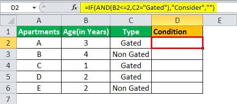
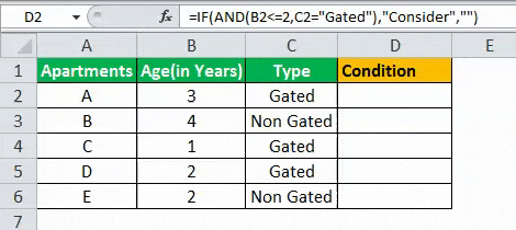
The table given below provides a list of apartments along with their age (in years) and type of society. Now we need to perform a comparative analysis for the apartments based on the age of the building and the type of society.
Here, we use the combination of less than equal (<=) to operator and the equal to (=) text functions in the condition to be demonstrated for IF AND function.
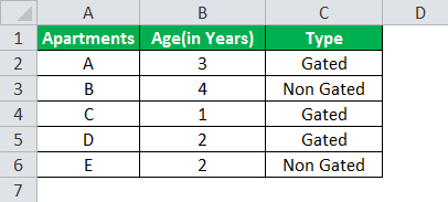
- The IF AND formula used to perform the analysis is stated as follows:
“=IF(AND(B2<=2,C2=“Gated”),“Consider”, “”)”
- The succeeding image shows the IF AND condition applied to perform the evaluation.
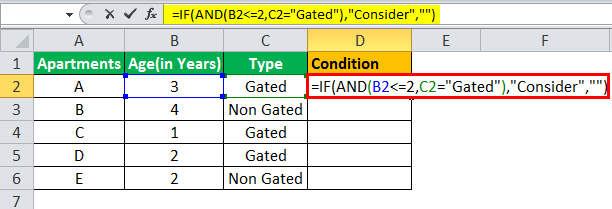
- Press “Enter” to get the answer.
- Drag the formula to find the results for all the apartments.
The results in the cell D of the above table shows that the IF AND formula will be performing one among the following:
- If both the arguments entered in the AND function is “true,” then the IF function will return that apartment to be “Consider.”
- If either of the arguments in the AND functionThe AND function in Excel is classified as a logical function; it returns TRUE if the specified conditions are met, otherwise it returns FALSE.read more is “false” or both the arguments entered are “false,” then the IF function will return a blank string.
The IF AND formula can also perform calculations based on whether the AND function returns “true” or “false,” apart from returning only the predefined text strings.
We will understand this concept with the help of the below-mentioned example.
Example #2
The given data tableA data table in excel is a type of what-if analysis tool that allows you to compare variables and see how they impact the result and overall data. It can be found under the data tab in the what-if analysis section.read more has the list of employee name along with their orders received, performance, and salaries. Calculate the employee hike (or bonus) based on two parameters–the number of orders received and performance.
The criteria to calculate the bonus is as follows.
- The number of orders received is greater than or equal to 200, and the performance is equal to “A.”
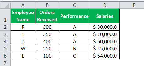
- The IF AND formula will be,
“=IF(AND(B2>=200,C2= “A”),D2*10%,D2*5%)”
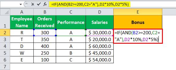
- Press “Enter” to get the final output. The bonus appears in cell E2.
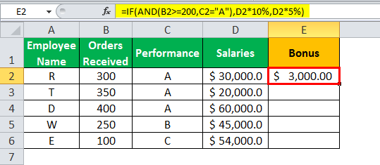
- Drag the formula to find the bonus of all employees.
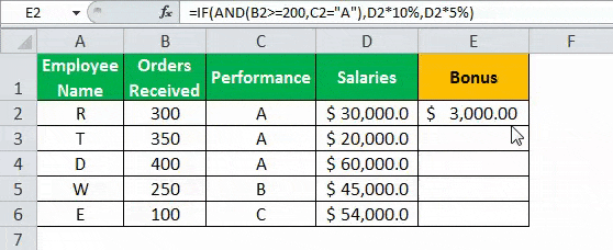
Based on these results, the IF formula does the following evaluation:
- If both the conditions are satisfied, the AND function returns “true,” then the bonus received is calculated as salary multiplied by 10%.
- If either one or both the conditions are found to be “false” by the AND function, then the bonus is calculated as salary multiplied by 5%.
Examples 1 and 2 have only two criteria to test and evaluate. Using multiple arguments or conditions to test them for “true” or “false” is also allowed.
Example #3
Let us evaluate multiple criteria and use AND function.
A table with five stocks and their parameter details including financial ratiosFinancial ratios are indications of a company’s financial performance. There are several forms of financial ratios that indicate the company’s results, financial risks, and operational efficiency, such as the liquidity ratio, asset turnover ratio, operating profitability ratios, business risk ratios, financial risk ratio, stability ratios, and so on.read more, such as ROCEReturn on Capital Employed (ROCE) is a metric that analyses how effectively a company uses its capital and, as a result, indicates long-term profitability. ROCE=EBIT/Capital Employed.read more, ROEReturn on Equity (ROE) represents financial performance of a company. It is calculated as the net income divided by the shareholders equity. ROE signifies the efficiency in which the company is using assets to make profit.read more, Debt to equityThe debt to equity ratio is a representation of the company’s capital structure that determines the proportion of external liabilities to the shareholders’ equity. It helps the investors determine the organization’s leverage position and risk level. read more, and PE ratioThe price to earnings (PE) ratio measures the relative value of the corporate stocks, i.e., whether it is undervalued or overvalued. It is calculated as the proportion of the current price per share to the earnings per share. read more is provided (shown in the below table). Using this data lets us test the condition to invest in suitable stocks. That is, using the parameters, let us analyze the stocks to derive the best investment horizonThe term «investment horizon» refers to the amount of time an investor is expected to hold an investment portfolio or a security before selling it. Depending on the need for funds and risk appetite, the investor may invest for a few days or hours to a few years or decades.read more, which is important for growth.
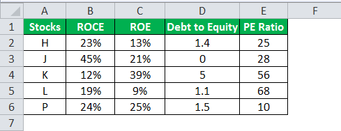
The following syntax is used where the conditions are applied to arrive at the result (shown in the below table).
“=IF(AND(B2>18%,C2>20%,D2<2,E2<30%),“Invest”,“”)”

- Press “Enter” to get the final output (Investment Criteria) of the above formula.

- Drag the formula to find the Investment Criteria.
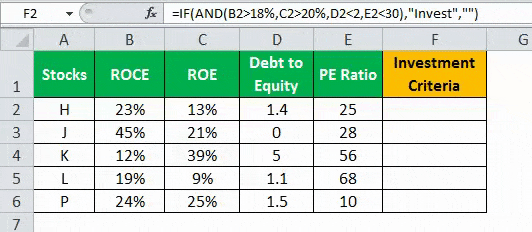
In the above data table, the AND function tests for the parameters using the operators. The resulting output generated by the IF formula is as follows:
- If all the four criteria mentioned in the AND function are tested and satisfied, then the IF function returns the “Invest” text string.
- If either one or more among the four conditions or all the four conditions fail to satisfy the AND function, then the IF function returns empty strings (“”).
The Characteristics of IF AND function
- The IF AND function does not differentiate between case-insensitive texts.
- The AND function can be used to evaluate up to 255 conditions for “true” or “false,” and the total formula length does not exceed 8192 characters.
- Text values or blank cells are given as an argument to test the conditions in AND function.
- The AND formula will return “#VALUE!” if there is no logical output found while evaluating the conditions.
- IF AND excel statement is a combination of two logical functions that tests and evaluates multiple conditions.
- The output of the AND function is based on, whether the IF function will return the value “true” or “false,” respectively.
- IF function is used to test a single criterion whereas, the AND function is used to test multiple criteria.
- The syntax of the IF AND formula is:
“=IF(AND (Condition 1,Condition 2,…),Value _if _True,Value _if _False)”
- The IF AND formula also performs a calculation based on whether the AND function is “true” or “false” apart from returning only the predefined text strings.
Frequently Asked Questions
1. How to use IF AND function in Excel?
The IF AND excel statement is the two logical functions often nested together.
Syntax:
“=IF(AND(Condition1,Condition2, value_if_true,vaue_if_false)”
The IF formula is used to test and compare the conditions expressed, along with the expected value. It provides the desired result if the condition is either “true” or “false.”
The AND formula is used to test multiple criteria. It returns “true” if all the given conditions are satisfied, or else returns “false.”
2. What is the IF AND function in Excel?
IF AND formula is applied as the combination of the two logical functions that enable the user to evaluate the multiple conditions. Based on the output of the AND function, the IF function returns the output “true” or “false.”
3. How to combine IF and AND functions in Excel?
To combine IF and AND functions, you need to replace the “condition_test” argument in the IF function with AND function.
“=IF(condition_test, value_if_true,vaue_if_false)”
“=IF(AND(Condition1,Condition2, value_if_true,vaue_if_false)”
In AND function we can use multiple conditions.
Recommended Articles
This has been a guide to IF AND function in Excel. Here we discuss how to use IF Formula combined with AND function along with examples and downloadable templates. You may also look at these useful functions in Excel –
- IF EXCEL FunctionIF function in Excel evaluates whether a given condition is met and returns a value depending on whether the result is “true” or “false”. It is a conditional function of Excel, which returns the result based on the fulfillment or non-fulfillment of the given criteria.
read more - Average IF Function
- SUMIF with Multiple CriteriaThe SUMIF (SUM+IF) with multiple criteria sums the cell values based on the conditions provided. The criteria are based on dates, numbers, and text. The SUMIF function works with a single criterion, while the SUMIFS function works with multiple criteria in excel.read more
- Nested If ConditionIn Excel, nested if function means using another logical or conditional function with the if function to test multiple conditions. For example, if there are two conditions to be tested, we can use the logical functions AND or OR depending on the situation, or we can use the other conditional functions to test even more ifs inside a single if.read more
Логическая функция ЕСЛИ в Экселе – одна из самых востребованных. Она возвращает результат (значение или другую формулу) в зависимости от условия.
Функция имеет следующий синтаксис.
ЕСЛИ(лог_выражение; значение_если_истина; [значение_если_ложь])
лог_выражение – это проверяемое условие. Например, A2<100. Если значение в ячейке A2 действительно меньше 100, то в памяти эксель формируется ответ ИСТИНА и функция возвращает то, что указано в следующем поле. Если это не так, в памяти формируется ответ ЛОЖЬ и возвращается значение из последнего поля.
значение_если_истина – значение или формула, которое возвращается при наступлении указанного в первом параметре события.
значение_если_ложь – это альтернативное значение или формула, которая возвращается при невыполнении условия. Данное поле не обязательно заполнять. В этом случае при наступлении альтернативного события функция вернет значение ЛОЖЬ.
Очень простой пример. Нужно проверить, превышают ли продажи отдельных товаров 30 шт. или нет. Если превышают, то формула должна вернуть «Ок», в противном случае – «Удалить». Ниже показан расчет с результатом.

Продажи первого товара равны 75, т.е. условие о том, что оно больше 30, выполняется. Следовательно, функция возвращает то, что указано в следующем поле – «Ок». Продажи второго товара менее 30, поэтому условие (>30) не выполняется и возвращается альтернативное значение, указанное в третьем поле. В этом вся суть функции ЕСЛИ. Протягивая расчет вниз, получаем результат по каждому товару.
Однако это был демонстрационный пример. Чаще формулу Эксель ЕСЛИ используют для более сложных проверок. Допустим, есть средненедельные продажи товаров и их остатки на текущий момент. Закупщику нужно сделать прогноз остатков через 2 недели. Для этого нужно от текущих запасов отнять удвоенные средненедельные продажи.

Пока все логично, но смущают минусы. Разве бывают отрицательные остатки? Нет, конечно. Запасы не могут быть ниже нуля. Чтобы прогноз был корректным, нужно отрицательные значения заменить нулями. Здесь отлично поможет формула ЕСЛИ. Она будет проверять полученное по прогнозу значение и если оно окажется меньше нуля, то принудительно выдаст ответ 0, в противном случае — результат расчета, т.е. некоторое положительное число. В общем, та же логика, только вместо значений используем формулу в качестве условия.

В прогнозе запасов больше нет отрицательных значений, что в целом очень неплохо.
Формулы Excel ЕСЛИ также активно используют в формулах массивов. Здесь мы не будем далеко углубляться. Заинтересованным рекомендую прочитать статью о том, как рассчитать максимальное и минимальное значение по условию. Правда, расчет в той статье более не актуален, т.к. в Excel 2016 появились функции МИНЕСЛИ и МАКСЕСЛИ. Но для примера очень полезно ознакомиться – пригодится в другой ситуации.
Формула ЕСЛИ в Excel – примеры нескольких условий
Довольно часто количество возможных условий не 2 (проверяемое и альтернативное), а 3, 4 и более. В этом случае также можно использовать функцию ЕСЛИ, но теперь ее придется вкладывать друг в друга, указывая все условия по очереди. Рассмотрим следующий пример.
Нескольким менеджерам по продажам нужно начислить премию в зависимости от выполнения плана продаж. Система мотивации следующая. Если план выполнен менее, чем на 90%, то премия не полагается, если от 90% до 95% — премия 10%, от 95% до 100% — премия 20% и если план перевыполнен, то 30%. Как видно здесь 4 варианта. Чтобы их указать в одной формуле потребуется следующая логическая структура. Если выполняется первое условие, то наступает первый вариант, в противном случае, если выполняется второе условие, то наступает второй вариант, в противном случае если… и т.д. Количество условий может быть довольно большим. В конце формулы указывается последний альтернативный вариант, для которого не выполняется ни одно из перечисленных ранее условий (как третье поле в обычной формуле ЕСЛИ). В итоге формула имеет следующий вид.

Комбинация функций ЕСЛИ работает так, что при выполнении какого-либо указанно условия следующие уже не проверяются. Поэтому важно их указать в правильной последовательности. Если бы мы начали проверку с B2<1, то условия B2<0,9 и B2<0,95 Excel бы просто «не заметил», т.к. они входят в интервал B2<1 который проверился бы первым (если значение менее 0,9, само собой, оно также меньше и 1). И тогда у нас получилось бы только два возможных варианта: менее 1 и альтернативное, т.е. 1 и более.
При написании формулы легко запутаться, поэтому рекомендуется смотреть на всплывающую подсказку.

В конце нужно обязательно закрыть все скобки, иначе эксель выдаст ошибку

Функция Excel ЕСЛИМН
Функция Эксель ЕСЛИ в целом хорошо справляется со своими задачами. Но вариант, когда нужно записывать длинную цепочку условий не очень приятный, т.к., во-первых, написать с первого раза не всегда получается (то условие укажешь неверно, то скобку не закроешь); во-вторых, разобраться при необходимости в такой формуле может быть непросто, особенно, когда условий много, а сами расчеты сложные.
В MS Excel 2016 появилась функция ЕСЛИМН, ради которой и написана вся эта статья. Это та же ЕСЛИ, только заточенная специально для проверки множества условий. Теперь не нужно сто раз писать ЕСЛИ и считать открытые скобки. Достаточно перечислить условия и в конце закрыть одну скобку.
Работает следующим образом. Возьмем пример выше и воспользуемся новой формулой Excel ЕСЛИМН.

Как видно, запись формулы выглядит гораздо проще и понятнее.
Стоит обратить внимание на следующее. Условия по-прежнему перечисляем в правильном порядке, чтобы не произошло ненужного перекрытия диапазонов. Последнее альтернативное условие, в отличие от обычной ЕСЛИ, также должно быть обязательно указано. В ЕСЛИ задается только альтернативное значение, которое наступает, если не выполняется ни одно из перечисленных условий. Здесь же нужно указать само условие, которое в нашем случае было бы B2>=1. Однако этого можно избежать, если в поле с условием написать ИСТИНА, указывая тем самым, что, если не выполняются ранее перечисленные условия, наступает ИСТИНА и возвращается последнее альтернативное значение.
Теперь вы знаете, как пользоваться функцией ЕСЛИ в Excel, а также ее более современным вариантом для множества условий ЕСЛИМН.
Поделиться в социальных сетях: