
IF function
The IF function is one of the most popular functions in Excel, and it allows you to make logical comparisons between a value and what you expect.
So an IF statement can have two results. The first result is if your comparison is True, the second if your comparison is False.
For example, =IF(C2=”Yes”,1,2) says IF(C2 = Yes, then return a 1, otherwise return a 2).

Use the IF function, one of the logical functions, to return one value if a condition is true and another value if it’s false.
IF(logical_test, value_if_true, [value_if_false])
For example:
-
=IF(A2>B2,»Over Budget»,»OK»)
-
=IF(A2=B2,B4-A4,»»)
|
Argument name |
Description |
|---|---|
|
logical_test (required) |
The condition you want to test. |
|
value_if_true (required) |
The value that you want returned if the result of logical_test is TRUE. |
|
value_if_false (optional) |
The value that you want returned if the result of logical_test is FALSE. |
Simple IF examples

-
=IF(C2=”Yes”,1,2)
In the above example, cell D2 says: IF(C2 = Yes, then return a 1, otherwise return a 2)

-
=IF(C2=1,”Yes”,”No”)
In this example, the formula in cell D2 says: IF(C2 = 1, then return Yes, otherwise return No)As you see, the IF function can be used to evaluate both text and values. It can also be used to evaluate errors. You are not limited to only checking if one thing is equal to another and returning a single result, you can also use mathematical operators and perform additional calculations depending on your criteria. You can also nest multiple IF functions together in order to perform multiple comparisons.

-
=IF(C2>B2,”Over Budget”,”Within Budget”)
In the above example, the IF function in D2 is saying IF(C2 Is Greater Than B2, then return “Over Budget”, otherwise return “Within Budget”)

-
=IF(C2>B2,C2-B2,0)
In the above illustration, instead of returning a text result, we are going to return a mathematical calculation. So the formula in E2 is saying IF(Actual is Greater than Budgeted, then Subtract the Budgeted amount from the Actual amount, otherwise return nothing).

-
=IF(E7=”Yes”,F5*0.0825,0)
In this example, the formula in F7 is saying IF(E7 = “Yes”, then calculate the Total Amount in F5 * 8.25%, otherwise no Sales Tax is due so return 0)
Note: If you are going to use text in formulas, you need to wrap the text in quotes (e.g. “Text”). The only exception to that is using TRUE or FALSE, which Excel automatically understands.
Common problems
|
Problem |
What went wrong |
|---|---|
|
0 (zero) in cell |
There was no argument for either value_if_true or value_if_False arguments. To see the right value returned, add argument text to the two arguments, or add TRUE or FALSE to the argument. |
|
#NAME? in cell |
This usually means that the formula is misspelled. |
Need more help?
You can always ask an expert in the Excel Tech Community or get support in the Answers community.

See Also
IF function — nested formulas and avoiding pitfalls
IFS function
Using IF with AND, OR and NOT functions
COUNTIF function
How to avoid broken formulas
Overview of formulas in Excel
Need more help?
Want more options?
Explore subscription benefits, browse training courses, learn how to secure your device, and more.
Communities help you ask and answer questions, give feedback, and hear from experts with rich knowledge.
What is IF Function in Excel?
IF function in Excel evaluates whether a given condition is met and returns a value depending on whether the result is “true” or “false”. It is a conditional function of Excel, which returns the result based on the fulfillment or non-fulfillment of the given criteria.
For example, the IF formula in Excel can be applied as follows:
“=IF(condition A,“value B”,“value C”)”
The IF excel function returns “value B” if condition A is met and returns “value C” if condition A is not met.
It is often used to make logical interpretations which help in decision-making.
Table of contents
- What is IF Function in Excel?
- Syntax of the IF Excel Function
- How to Use IF Function in Excel?
- Example #1
- Example #2
- Example #3
- Example #4
- Example #5
- Guidelines for the Multiple IF Statements
- Frequently Asked Question
- IF Excel Function Video
- Recommended Articles
Syntax of the IF Excel Function
The syntax of the IF function is shown in the following image:

The IF excel function accepts the following arguments:
- Logical_test: It refers to the condition to be evaluated. The condition can be a value or a logical expression.
- Value_if_true: It is the value returned as a result when the condition is “true”.
- Value_if_false: It is the value returned as a result when the condition is “false”.
In the formula, the “logical_test” is a required argument, whereas the “value_if_true” and “value_if_false” are optional arguments.
The IF formula uses logical operators to evaluate the values in a range of cells. The following table shows the different logical operatorsLogical operators in excel are also known as the comparison operators and they are used to compare two or more values, the return output given by these operators are either true or false, we get true value when the conditions match the criteria and false as a result when the conditions do not match the criteria.read more and their meaning.
| Operator | Meaning |
|---|---|
| = | Equal to |
| > | Greater than |
| >= | Greater than or equal to |
| < | Less than |
| <= | Less than or equal to |
| <> | Not equal to |
How to Use IF Function in Excel?
Let us understand the working of the IF function with the help of the following examples in Excel.
You can download this IF Function Excel Template here – IF Function Excel Template
Example #1
If there is no oxygen on a planet, life is impossible. If oxygen is available on a planet, then life is possible. The following table shows a list of planets in column A and the information on the availability of oxygen in column B. We have to find the planets where life is possible, based on the condition of oxygen availability.

Let us apply the IF formula to cell C2 to find out whether life is possible on the planets listed in the table.
The IF formula is stated as follows:
“=IF(B2=“Yes”, “Life is Possible”, “Life is Not Possible”)
The succeeding image shows the IF formula applied to cell C2.

The subsequent image shows how the IF formula is applied to the range of cells C2:C5.

Drag the cells to view the output of all the planets.

The output in the below worksheet shows life is possible on the planet Earth.
Flow Chart of Generic IF Excel Function

The IF Function Flow Chart for Mars (Example #1)

The flow of IF function flowchart for Jupiter and Venus is the same as the IF function flowchart for Mars (Example #1).
The IF Function Flow Chart for Earth

Hence, the IF excel function allows making logical comparisons between values. The modus operandi of the IF function is stated as: If something is true, then do something; otherwise, do something else.
Example #2
The following table shows a list of years. We want to find out if the given year is a leap year or not.
A leap year has 366 days; the extra day is the 29th of February. The criteria for a leap year are stated as follows:
- The year will be exactly divisible by 4 and not exactly be divisible by 100 or
- The year will be exactly divisible by 400.

In this example, we will use the IF function along with the AND, OR, and MOD functions to find the leap years.
We use the MOD function to find a remainder after a dividend is divided by a divisor.
The AND functionThe AND function in Excel is classified as a logical function; it returns TRUE if the specified conditions are met, otherwise it returns FALSE.read more evaluates both the conditions of the leap years for the value “true”. The OR functionThe OR function in Excel is used to test various conditions, allowing you to compare two values or statements in Excel. If at least one of the arguments or conditions evaluates to TRUE, it will return TRUE. Similarly, if all of the arguments or conditions are FALSE, it will return FASLE.read more evaluates either of the condition for the value “true”.
We will apply the MOD function to the conditions as follows:
If MOD(year,4)=0 and MOD(year,100)<>(is not equal to) 0, then the year is a leap year.
or
If MOD(year,400)=0, then the year is a leap year; otherwise, the year is not a leap year.
The IF formula is stated as follows:
“=IF(OR(AND((MOD(year,4)=0),(MOD(year,100)<>0)),(MOD(year,400)=0)),“Leap Year”, “Not A Leap Year”)”
The argument “year” refers to a reference value.
The following images show the output of the IF formula applied in the range of cells.


The following image shows how the IF formula is applied to the range of cells B2:B18.

The succeeding table shows the years 1960, 2028, and 2148 as leap years and the remaining as non-leap years.

The result of the IF excel formula is displayed for the range of cells B2:B18 in the following image.

Example #3
The succeeding table shows a list of drivers and the directions they undertook to reach the destination. It is preceded by an image of the road intersection explaining the turns taken by the drivers and their destinations. The right turn leads to town B, and the left turn leads to town C. Identify the driver’s destination to town B and town C.
Road Intersection Image


Let us apply the IF excel function to find the destination. Here, the condition is mentioned as follows:
- If the driver turns right, he/she reaches town B.
- If the driver turns left, he/she reaches town C.
We use the following IF formula to find the destination:
“=IF(B2=“Left”, “Town C”, “Town B”)”
The succeeding image shows the output of the IF formula applied to cell C2.

Drag the cells to use the formula in the range C2:C11. Finally, we get the destinations of each driver for their turning movements.
The below image displays the IF formula applied to the range.

The output of the IF formula and the destinations are displayed in the succeeding image.

The result shows that six drivers reached town C, and the remaining four have reached town B.
Example #4
The following table shows a list of items and their inventory levels. We want to check if the specific item is available in the inventory or not using the IF function.

Let us list the name of items in column A and the number of items in column B. The list of data to be validated for the entire items list is shown in the cell E2 of the below image.

We use the Excel IF along with the VLOOKUP functionThe VLOOKUP excel function searches for a particular value and returns a corresponding match based on a unique identifier. A unique identifier is uniquely associated with all the records of the database. For instance, employee ID, student roll number, customer contact number, seller email address, etc., are unique identifiers.
read more to check the availability of the items in the inventory.
The VLOOKUP function looks up the values referring to the number of items, and the IF function will check whether the item number is greater than zero or not.
We will apply the following IF formula in the F2 cell:
“=IF(VLOOKUP(E2,A2:B11,2,0)=0, “Item Not Available”,“Item Available”)”
If the lookup value of an item is equal to 0, then the item is not available; else, the item is available.
The succeeding image shows the result of the IF formula in the cell F2.

Select “bat” in the E2 item cell to know whether the item is available or not in the inventory (as shown in the following image).

Example #5
The following table shows the list of students and their marks. The grade criteria are provided based on the marks obtained by the students. We want to find the grade of each student in the list.

We apply the Nested IF in Excel since we have multiple criteria to find and decide each student’s grade.
The Nesting of IF function uses the IF function inside another IF formula when multiple conditions are to be fulfilled.
The syntax of Nesting of IF function is stated as follows:
“=IF( condition1, value_if_true1, IF( condition2, value_if_true2, value_if_false2 ))”
The succeeding table represents the range of scores and the grades, respectively.

Let us apply the multiple IF conditions with AND function in the below-nested formula to find out the grade of the students:
“=IF((B2>=95),“A”,IF(AND(B2>=85,B2<=94),“B”,IF(AND(B2>=75,B2<=84),“C”,IF(AND(B2>=61,B2<=74),“D”,“F”))))”
The IF function checks the logical condition as shown in the formula below:
“=IF(logical_test, [value_if_true],[value_if_false])”
We will split the above-mentioned nested formula and check the IF statements as shown below:
First Logical Test: B2>=95
If the formula returns,
- Value_if_true, execute: “A” (Grade A) else(comma) enter value_if_false
- Value_if_false, then the formula finds another IF condition and enter IF condition
Second Logical Test: B2>=85(logical expression 1) and B2<=94(logical expression 2)
(We use AND function to check the multiple logical expressions as the two given conditions are to be evaluated for “true.”)
If the formula returns,
- Value_if_true, execute: “B” (Grade B) else(comma) enter value_if_false
- Value_if_false, then the formula finds another IF condition and enter IF condition
Third Logical Test: B2>=75(logical expression 1) and B2<=84(logical expression 2)
(We use AND function to check the multiple logical expressions as the two given conditions are to be evaluated for “true.”)
If the formula returns,
- Value_if_true, execute: “C” (Grade C) else(comma) enter value_if_false
- value_if_false, then the formula finds another IF condition and enter IF condition
Fourth Logical Test: B2>=61(logical expression 1) and B2<=74(logical expression 2)
(We use AND function to check the multiple logical expressions as the two given conditions are to be evaluated for “true.”)
If the formula returns,
- Value_if_true, execute: “D” (Grade D) else(comma) enter value_if_false
- Value_if_false, execute: “F” (Grade F)
- Finally, close the parenthesis.
The below image displays the output of the IF formula applied to the range.

The succeeding image shows the IF nested formula applied to the range.

The grades of the students are listed in the following table.

Guidelines for the Multiple IF Statements
The guidelines for the multiple IF statements are listed as follows:
- Use nested IF function to a limited extent as multiple IF statements require a great deal of thought to be accurate.
- Multiple IF statementsIn Excel, multiple IF conditions are IF statements that are contained within another IF statement. They are used to test multiple conditions at the same time and return distinct values. Additional IF statements can be included in the ‘value if true’ and ‘value if false’ arguments of a standard IF formula.read more require multiple parentheses (), which is often difficult to manage. Excel provides a way to check the color of each opening and closing parenthesis to avoid this situation. The last closing parenthesis color will always be black, denoting the end of the formula statement.
- Whenever we pass a string value for the arguments “value_if_true” and “value_if_false” or test a reference against a string value, enclose the string value in double quotes. Passing a string value without quotes will result in “#NAME?” error.
Frequently Asked Question
1. What is the IF function in Excel?
The Excel IF function is a logical function that checks the given criteria and returns one value for a “true” and another value for a “false” result.
The syntax of the IF function is stated as follows:
“=IF(logical_test, [value_if_true], [value_if_false])”
The arguments are as follows:
1. Logical_test – It refers to a value or condition that is tested.
2. Value_if_true – It is the value returned when the condition logical_test is “true.”
3. Value_if_false – It is the value returned when the condition logical_test is “false.”
The “logical_test” is a required argument, whereas the “value_if_true” and “value_if_false” are optional arguments.
2. How to use the IF Excel function with multiple conditions?
The IF Excel statement for multiple conditions is created by using multiple IF functions in a single formula.
The syntax of IF function with multiple conditions is stated as follows:
“=IF (condition 1_“true”, do something, IF (condition 2_“true”, do something, IF (condition 3_ “true”, do something, else do something)))”
3. How to use the function IFERROR in Excel?
IF Excel Function Video
Recommended Articles
This has been a guide to the IF function in Excel. Here we discuss how to use the IF function along with examples and downloadable templates. You may also look at these useful functions –
- What is the Logical Test in Excel?A logical test in Excel results in an analytical output, either true or false. The equals to operator, “=,” is the most commonly used logical test.read more
- “Not Equal to” in Excel“Not Equal to” argument in excel is inserted with the expression <>. The two brackets posing away from each other command excel of the “Not Equal to” argument, and the user then makes excel checks if two values are not equal to each other.read more
- Data Validation ExcelThe data validation in excel helps control the kind of input entered by a user in the worksheet.read more
In this tutorial, we will learn about the IF function in Excel. Along with IF, the AND and OR functions are important formulas too. A nested IF simply means multiple IF functions in a single syntax.
Introducing IF Function in Excel
Let’s get started with this easy guide to using the IF function and all its related functions in Microsoft Excel, step-by-step with supporting images and examples.
1. IF Function
To learn to use the IF function, we will take an example of a mark list of students below.

Our goal is to find out which student has passed or failed and what are their grades. Of course, it would be a tedious task to find out pass or fail results and grades for each student in this list.
To ease our task, we have IF functions for that matter. The IF function will automatically identify if a student has passed or failed based on the criteria you provide to it.
It will automatically mark a student as “Pass” if he/she has scored above the minimum pass mark and mark a student as “Fail” if he/she has scored below the minimum pass mark.
The IF function automatically assigns the appropriate grades to students based on their marks if you command it.
Here is a glimpse of how the IF function helps you out with assigning grades and marking “Pass” or “Fail”.

Steps to use IF function in Excel
We have allotted certain grades and marked them as Pass or Fail to students based on the percentages they have secured in their exams, with the help of the IF function.
1. Using the IF function in Excel to identify passed/failed students
Let’s learn how we can use the IF formula to achieve this. We will use the same example. We take the minimum passing percentage as 34%.

- Find out the percentage of total marks of every student.
- Create a new column named “Pass/Fail”.
- In the blank cell below the title, type the IF formula as follows next.
- Type =IF( and select the first student’s percentage and type >=34.
- Put a comma and move to the next argument named [value_if_true]. This means you’re being asked to put a value to be displayed if the above condition is true. Remember these arguments are case sensitive.
- Once you have put a comma, type “Pass”.
- Put a comma and move to the next argument named [value_if_false] to display a value when the above condition is false. This field is optional in most cases but we need a false value because it is a mark list.
- Close the bracket and hit ENTER.

You can see that the formula is displaying “Pass” for the first student because she has secured above 34%.
- Double-click or drag the cell from the right corner below to autofill the formula to all the students below.

Recommended read: How to Autofill in Excel?
2. Nested IF Function
Now, let us start assigning grades to all students.
We are going to be using multiple IF functions in a single syntax this time to provide multiple criteria to the IF function. This is called Nested IF in Excel.
However, there is no specific function named “Nested IF” in Excel, it is simply that this behavior has been given a name i.e., Nested IF.
Before we proceed further, we need to first make a table that displays a grading class for each grade. Here is an example below.

- Create a new column named “Grade”.
- Type the IF function in a blank cell below the title as follows.
- Type =IF( and now type AE118>=85,”A”,IF(AE118>=70,”B”,IF(AE118>=55,”C”,IF(AE118>=34,”D”,IF(AE118<=33,”Fail”.

- Note that AE118 is our cell address for the first student’s percentage. It will be different in your case. Refer to the image above to make sense of the formula.
- The formula simply states- if percentage marks are above and equal to 85 then give “A”, if percentage marks are above and equal to 70 then give “B”, and so on and so forth. For the last condition, we have applied the condition- if the marks are less than or equal to 33 then give “Fail”.
- For the last IF statement, you can either put the result as “Fail” or “E” as you like.
- Now, note that we will close the formula with 5 brackets for this example as we have used a total of 5 IF formulas.

- Hit ENTER to complete the formula.

You can now see that the formula has been applied to the first entry and the result is B because the student has secured 72.5% which is less than 75%. This means the nested Ifs are working correctly.
- Now drag the cell from the lower right corner to autofill the formula to the rest of the entries.

You can see that we now have grades and pass/fail markings for every student on the list successfully.
3. IF with AND in Excel
Let us learn the IF formula with the AND function in a single syntax with a minor example.

When you have two or more distinct conditions to be used together, you can use the IF function with AND in Excel.
While nested IFs will also work, using AND function will save your time as it is shorter to type. So, let’s get started.
Our goal is to identify currencies with revenues greater than 20,000 and less than 50,000 and mark them as “Good”.
- Type =IF(AND( because we are using the IF with AND function.
- Select the first cell under Revenue, and type >20000.
- Put a comma and select the first cell under Revenue again and type <50000.
- Now, close the bracket to complete the AND function. We’re still working on the IF function so do not put two brackets.
- We come back to the IF function as soon as we close the AND function. Now put the values to be displayed if the condition is true or false.
- Put a comma to move to the argument [value_if_true] and type “Good”.
- You can provide a result in the [value_if_false] argument, but it is completely optional. If nothing is provided then the cells will display FALSE if the condition is false. But if you want the cells to remain blank simply put “” (two double quotation marks) in this argument.
- Close the bracket to complete the IF function as well.

This is how the syntax should look like before pressing ENTER.
- Hit ENTER to view results and drag the cell down to autofill the formula to the rest of the cells.

There are only two such cells for which the condition is true and the result is being displayed as “Good” for them and the rest of the cells are blank. This means the formula is working correctly.
4. IF with OR in Excel
Using the OR function with the IF function will give results for either of the conditions that are true.
- Type =IF(OR(.
- Select the first cell under Revenue and type >=20000.
- Put a comma and select the first cell under Revenue again and type <=50000.
- Now, close the bracket to complete the OR function. We’re still working on the IF function so do not put two brackets.
- Coming back to the IF function, we now put the values to be displayed if the condition is true or false.
- Put a comma to move to the argument [value_if_true] and type “Flag”.
- Put a comma to move to the argument [value_if_false] and type “”.

This is how the syntax should look like before pressing ENTER.
- Close the bracket to complete the OR function and hit ENTER.
- Drag the cell below to get the results for the rest.

The formula is true for all entries and so it is displaying “Flag” for all of them. This is because all the values are either lower than 50,000 or greater than 20,000.
Conclusion
This was all about IF functions and other related functions to the IF function that are AND and OR functions.
Reference: ExcelJet
![]()
Excel If Cell Contains Text

Excel If Cell Contains Text Then Formula helps you to return the output when a cell have any text or a specific text. You can check if a cell contains a some string or text and produce something in other cell. For Example you can check if a cell A1 contains text ‘example text’ and print Yes or No in Cell B1. Following are the example Formulas to check if Cell contains text then return some thing in a Cell.
If Cell Contains Text
Here are the Excel formulas to check if Cell contains specific text then return something. This will return if there is any string or any text in given Cell. We can use this simple approach to check if a cell contains text, specific text, string, any text using Excel If formula. We can use equals to operator(=) to compare the strings .
If Cell Contains Text Then TRUE
Following is the Excel formula to return True if a Cell contains Specif Text. You can check a cell if there is given string in the Cell and return True or False.
The formula will return true if it found the match, returns False of no match found.
If Cell Contains Partial Text
We can return Text If Cell Contains Partial Text. We use formula or VBA to Check Partial Text in a Cell.
Find for Case Sensitive Match:
We can check if a Cell Contains Partial Text then return something using Excel Formula. Following is a simple example to find the partial text in a given Cell. We can use if your want to make the criteria case sensitive.
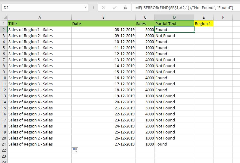
- Here, Find Function returns the finding position of the given string
- Use Find function is Case Sensitive
- IsError Function check if Find Function returns Error, that means, string not found
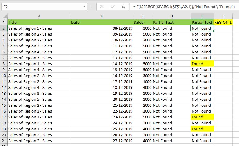
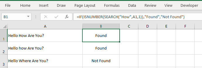
Search for Not Case Sensitive Match:
We can use Search function to check if Cell Contains Partial Text. Search function useful if you want to make the checking criteria Not Case Sensitive.
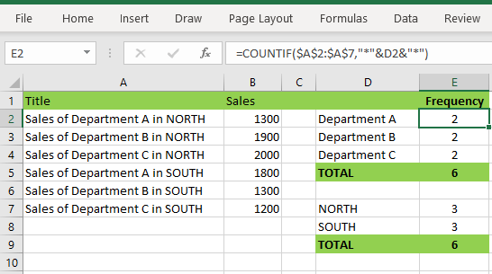
If Range of Cells Contains Text
We can check for the strings in a range of cells. Here is the formula to find If Range of Cells Contains Text. We can use Count If Formula to check the excel if range of cells contains specific text and return Text.
- CountIf function counts the number of cells with given criteria
- We can use If function to return the required Text
- Formula displays the Text ‘Range Contains Text” if match found
- Returns “Text Not Found in the Given Range” if match not found in the specified range
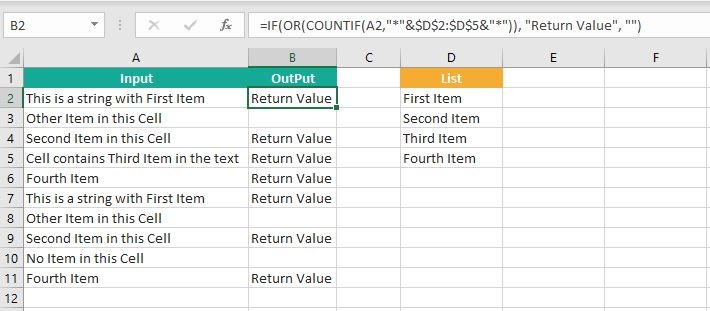
If Cells Contains Text From List
Below formulas returns text If Cells Contains Text from given List. You can use based on your requirement.
VlookUp to Check If Cell Contains Text from a List:
We can use VlookUp function to match the text in the Given list of Cells. And return the corresponding values.
- Check if a List Contains Text:
=IF(ISERR(VLOOKUP(F1,A1:B21,2,FALSE)),”False:Not Contains”,”True: Text Found”) - Check if a List Contains Text and Return Corresponding Value:
=VLOOKUP(F1,A1:B21,2,FALSE) - Check if a List Contains Partial Text and Return its Value:
=VLOOKUP(“*”&F1&”*”,A1:B21,2,FALSE)
If Cell Contains Text Then Return a Value
We can return some value if cell contains some string. Here is the the the Excel formula to return a value if a Cell contains Text. You can check a cell if there is given string in the Cell and return some string or value in another column.
The formula will return true if it found the match, returns False of no match found. can
Excel if cell contains word then assign value
You can replace any word in the following formula to check if cell contains word then assign value.
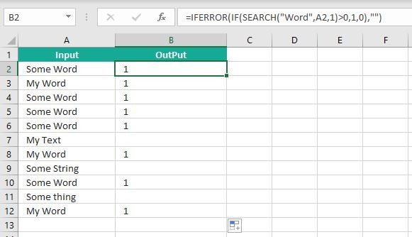
Search function will check for a given word in the required cell and return it’s position. We can use If function to check if the value is greater than 0 and assign a given value (example: 1) in the cell. search function returns #Value if there is no match found in the cell, we can handle this using IFERROR function.
Count If Cell Contains Text
We can check If Cell Contains Text Then COUNT. Here is the Excel formula to Count if a Cell contains Text. You can count the number of cells containing specific text.
The formula will Sum the values in Column B if the cells of Column A contains the given text.
Count If Cell Contains Partial Text
We can count the cells based on partial match criteria. The following Excel formula Counts if a Cell contains Partial Text.
- We can use the CountIf Function to Count the Cells if they contains given String
- Wild-card operators helps to make the CountIf to check for the Partial String
- Put Your Text between two asterisk symbols (*YourText*) to make the criteria to find any where in the given Cell
- Add Asterisk symbol at end of your text (YourText*) to make the criteria to find your text beginning of given Cell
- Place Asterisk symbol at beginning of your text (*YourText) to make the criteria to find your text end of given Cell
If Cell contains text from list then return value
Here is the Excel Formula to check if cell contains text from list then return value. We can use COUNTIF and OR function to check the array of values in a Cell and return the given Value. Here is the formula to check the list in range D2:D5 and check in Cell A2 and return value in B2.
If Cell Contains Text Then SUM
Following is the Excel formula to Sum if a Cell contains Text. You can total the cell values if there is given string in the Cell. Here is the example to sum the column B values based on the values in another Column.
The formula will Sum the values in Column B if the cells of Column A contains the given text.

Sum If Cell Contains Partial Text
Use SumIfs function to Sum the cells based on partial match criteria. The following Excel formula Sums the Values if a Cell contains Partial Text.
- SUMIFS Function will Sum the Given Sum Range
- We can specify the Criteria Range, and wild-card expression to check for the Partial text
- Put Your Text between two asterisk symbols (*YourText*) to Sum the Cells if the criteria to find any where in the given Cell
- Add Asterisk symbol at end of your text (YourText*) to Sum the Cells if the criteria to find your text beginning of given Cell
- Place Asterisk symbol at beginning of your text (*YourText) to Sum the Cells if criteria to find your text end of given Cell
VBA to check if Cell Contains Text
Here is the VBA function to find If Cells Contains Text using Excel VBA Macros.
If Cell Contains Partial Text VBA
We can use VBA to check if Cell Contains Text and Return Value. Here is the simple VBA code match the partial text. Excel VBA if Cell contains partial text macros helps you to use in your procedures and functions.
MsgBox CheckIfCellContainsPartialText(Cells(2, 1), “Region 1”)
End Sub
Function CheckIfCellContainsPartialText(ByVal cell As Range, ByVal strText As String) As Boolean
If InStr(1, cell.Value, strText) > 0 Then CheckIfCellContainsPartialText = True
End Function
- CheckIfCellContainsPartialText VBA Function returns true if Cell Contains Partial Text
- inStr Function will return the Match Position in the given string
If Cell Contains Text Then VBA MsgBox
Here is the simple VBA code to display message box if cell contains text. We can use inStr Function to search for the given string. And show the required message to the user.
If InStr(1, Cells(2, 1), “Region 3”) > 0 Then blnMatch = True
If blnMatch = True Then MsgBox “Cell Contains Text”
End Sub
- inStr Function will return the Match Position in the given string
- blnMatch is the Boolean variable becomes True when match string
- You can display the message to the user if a Range Contains Text
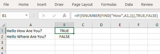
Which function returns true if cell a1 contains text?
You can use the Excel If function and Find function to return TRUE if Cell A1 Contains Text. Here is the formula to return True.
Which function returns true if cell a1 contains text value?
You can use the Excel If function with Find function to return TRUE if a Cell A1 Contains Text Value. Below is the formula to return True based on the text value.
Share This Story, Choose Your Platform!
7 Comments
-
Meghana
December 27, 2019 at 1:42 pm — ReplyHi Sir,Thank you for the great explanation, covers everything and helps use create formulas if cell contains text values.
Many thanks! Meghana!!
-
Max
December 27, 2019 at 4:44 pm — ReplyPerfect! Very Simple and Clear explanation. Thanks!!
-
Mike Song
August 29, 2022 at 2:45 pm — ReplyI tried this exact formula and it did not work.
-
Theresa A Harding
October 18, 2022 at 9:51 pm — Reply -
Marko
November 3, 2022 at 9:21 pm — ReplyHi
Is possible to sum all WA11?
(A1) WA11 4
(A2) AdBlue 1, WA11 223
(A3) AdBlue 3, WA11 32, shift 4
… and everything is in one column.
Thanks you very much for your help.
Sincerely Marko
-
Mike
December 9, 2022 at 9:59 pm — ReplyThank you for the help. The formula =OR(COUNTIF(M40,”*”&Vendors&”*”)) will give “TRUE” when some part of M40 contains a vendor from “Vendors” list. But how do I get Excel to tell which vendor it found in the M40 cell?
-
PNRao
December 18, 2022 at 6:05 am — ReplyPlease describe your question more elaborately.
Thanks!
-
© Copyright 2012 – 2020 | Excelx.com | All Rights Reserved
Page load link
Excel has a number of formulas that help you use your data in useful ways. For example, you can get an output based on whether or not a cell meets certain specifications. Right now, we’ll focus on a function called “if cell contains, then”. Let’s look at an example.
Jump To Specific Section:
- Explanation: If Cell Contains
- If cell contains any value, then return a value
- If cell contains text/number, then return a value
- If cell contains specific text, then return a value
- If cell contains specific text, then return a value (case-sensitive)
- If cell does not contain specific text, then return a value
- If cell contains one of many text strings, then return a value
- If cell contains several of many text strings, then return a value
Excel Formula: If cell contains
Generic formula
=IF(ISNUMBER(SEARCH("abc",A1)),A1,"")
Summary
To test for cells that contain certain text, you can use a formula that uses the IF function together with the SEARCH and ISNUMBER functions. In the example shown, the formula in C5 is:
=IF(ISNUMBER(SEARCH("abc",B5)),B5,"")
If you want to check whether or not the A1 cell contains the text “Example”, you can run a formula that will output “Yes” or “No” in the B1 cell. There are a number of different ways you can put these formulas to use. At the time of writing, Excel is able to return the following variations:
- If cell contains any value
- If cell contains text
- If cell contains number
- If cell contains specific text
- If cell contains certain text string
- If cell contains one of many text strings
- If cell contains several strings
Using these scenarios, you’re able to check if a cell contains text, value, and more.
Explanation: If Cell Contains
One limitation of the IF function is that it does not support Excel wildcards like «?» and «*». This simply means you can’t use IF by itself to test for text that may appear anywhere in a cell.
One solution is a formula that uses the IF function together with the SEARCH and ISNUMBER functions. For example, if you have a list of email addresses, and want to extract those that contain «ABC», the formula to use is this:
=IF(ISNUMBER(SEARCH("abc",B5)),B5,""). Assuming cells run to B5
If «abc» is found anywhere in a cell B5, IF will return that value. If not, IF will return an empty string («»). This formula’s logical test is this bit:
ISNUMBER(SEARCH("abc",B5))
Read article: Excel efficiency: 11 Excel Formulas To Increase Your Productivity
Using “if cell contains” formulas in Excel
The guides below were written using the latest Microsoft Excel 2019 for Windows 10. Some steps may vary if you’re using a different version or platform. Contact our experts if you need any further assistance.
1. If cell contains any value, then return a value
This scenario allows you to return values based on whether or not a cell contains any value at all. For example, we’ll be checking whether or not the A1 cell is blank or not, and then return a value depending on the result.
- Select the output cell, and use the following formula: =IF(cell<>»», value_to_return, «»).
- For our example, the cell we want to check is A2, and the return value will be No. In this scenario, you’d change the formula to =IF(A2<>»», «No», «»).
- Since the A2 cell isn’t blank, the formula will return “No” in the output cell. If the cell you’re checking is blank, the output cell will also remain blank.
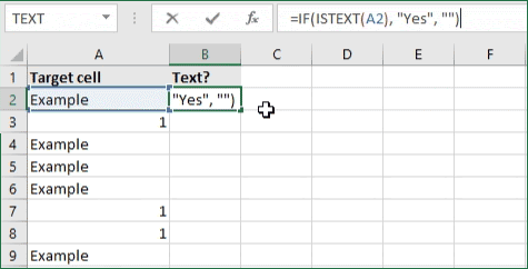
2. If cell contains text/number, then return a value
With the formula below, you can return a specific value if the target cell contains any text or number. The formula will ignore the opposite data types.
Check for text
- To check if a cell contains text, select the output cell, and use the following formula: =IF(ISTEXT(cell), value_to_return, «»).
- For our example, the cell we want to check is A2, and the return value will be Yes. In this scenario, you’d change the formula to =IF(ISTEXT(A2), «Yes», «»).

- Because the A2 cell does contain text and not a number or date, the formula will return “Yes” into the output cell.
Check for a number or date
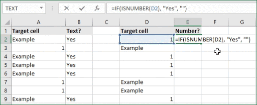
- To check if a cell contains a number or date, select the output cell, and use the following formula: =IF(ISNUMBER(cell), value_to_return, «»).
- For our example, the cell we want to check is D2, and the return value will be Yes. In this scenario, you’d change the formula to =IF(ISNUMBER(D2), «Yes», «»).

- Because the D2 cell does contain a number and not text, the formula will return “Yes” into the output cell.
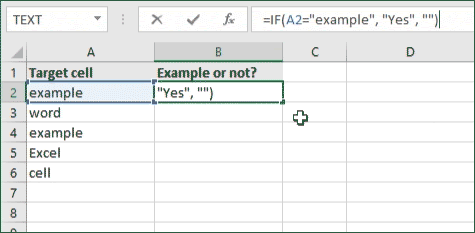
3. If cell contains specific text, then return a value
To find a cell that contains specific text, use the formula below.
- Select the output cell, and use the following formula: =IF(cell=»text», value_to_return, «»).
- For our example, the cell we want to check is A2, the text we’re looking for is “example”, and the return value will be Yes. In this scenario, you’d change the formula to =IF(A2=»example», «Yes», «»).

- Because the A2 cell does consist of the text “example”, the formula will return “Yes” into the output cell.
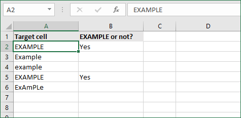
4. If cell contains specific text, then return a value (case-sensitive)
To find a cell that contains specific text, use the formula below. This version is case-sensitive, meaning that only cells with an exact match will return the specified value.
- Select the output cell, and use the following formula: =IF(EXACT(cell,»case_sensitive_text»), «value_to_return», «»).
- For our example, the cell we want to check is A2, the text we’re looking for is “EXAMPLE”, and the return value will be Yes. In this scenario, you’d change the formula to =IF(EXACT(A2,»EXAMPLE»), «Yes», «»).
- Because the A2 cell does consist of the text “EXAMPLE” with the matching case, the formula will return “Yes” into the output cell.
5. If cell does not contain specific text, then return a value
The opposite version of the previous section. If you want to find cells that don’t contain a specific text, use this formula.
- Select the output cell, and use the following formula: =IF(cell=»text», «», «value_to_return»).
- For our example, the cell we want to check is A2, the text we’re looking for is “example”, and the return value will be No. In this scenario, you’d change the formula to =IF(A2=»example», «», «No»).
- Because the A2 cell does consist of the text “example”, the formula will return a blank cell. On the other hand, other cells return “No” into the output cell.
6. If cell contains one of many text strings, then return a value
This formula should be used if you’re looking to identify cells that contain at least one of many words you’re searching for.
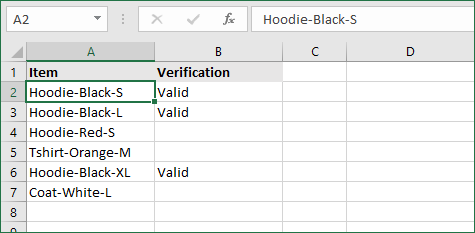
- Select the output cell, and use the following formula: =IF(OR(ISNUMBER(SEARCH(«string1», cell)), ISNUMBER(SEARCH(«string2», cell))), value_to_return, «»).
- For our example, the cell we want to check is A2. We’re looking for either “tshirt” or “hoodie”, and the return value will be Valid. In this scenario, you’d change the formula to =IF(OR(ISNUMBER(SEARCH(«tshirt»,A2)),ISNUMBER(SEARCH(«hoodie»,A2))),»Valid «,»»).
- Because the A2 cell does contain one of the text values we searched for, the formula will return “Valid” into the output cell.
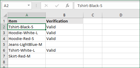
To extend the formula to more search terms, simply modify it by adding more strings using ISNUMBER(SEARCH(«string», cell)).
7. If cell contains several of many text strings, then return a value
This formula should be used if you’re looking to identify cells that contain several of the many words you’re searching for. For example, if you’re searching for two terms, the cell needs to contain both of them in order to be validated.
- Select the output cell, and use the following formula: =IF(AND(ISNUMBER(SEARCH(«string1»,cell)), ISNUMBER(SEARCH(«string2″,cell))), value_to_return,»»).
- For our example, the cell we want to check is A2. We’re looking for “hoodie” and “black”, and the return value will be Valid. In this scenario, you’d change the formula to =IF(AND(ISNUMBER(SEARCH(«hoodie»,A2)),ISNUMBER(SEARCH(«black»,A2))),»Valid «,»»).
- Because the A2 cell does contain both of the text values we searched for, the formula will return “Valid” to the output cell.
Final thoughts
We hope this article was useful to you in learning how to use “if cell contains” formulas in Microsoft Excel. Now, you can check if any cells contain values, text, numbers, and more. This allows you to navigate, manipulate and analyze your data efficiently.
We’re glad you’re read the article up to here  Thank you
You may also like
» How to use NPER Function in Excel
» How to Separate First and Last Name in Excel
» How to Calculate Break-Even Analysis in Excel
The logical IF statement in Excel is used for the recording of certain conditions. It compares the number and / or text, function, etc. of the formula when the values correspond to the set parameters, and then there is one record, when do not respond — another.
Logic functions — it is a very simple and effective tool that is often used in practice. Let us consider it in details by examples.
The syntax of the function «IF» with one condition
The operation syntax in Excel is the structure of the functions necessary for its operation data.
=IF(boolean;value_if_TRUE;value_if_FALSE)
Let us consider the function syntax:
- Boolean – what the operator checks (text or numeric data cell).
- Value_if_TRUE – what will appear in the cell when the text or numbers correspond to a predetermined condition (true).
- Value_if_FALSE – what appears in the box when the text or the number does not meet the predetermined condition (false).
Example:

Logical IF functions.
The operator checks the A1 cell and compares it to 20. This is a «Boolean». When the contents of the column is more than 20, there is a true legend «greater 20». In the other case it’s «less or equal 20».
Attention! The words in the formula need to be quoted. For Excel to understand that you want to display text values.
Here is one more example. To gain admission to the exam, a group of students must successfully pass a test. The results are listed in a table with columns: a list of students, a credit, an exam.

The statement IF should check not the digital data type but the text. Therefore, we prescribed in the formula В2= «done» We take the quotes for the program to recognize the text correctly.
The function IF in Excel with multiple conditions
Usually one condition for the logic function is not enough. If you need to consider several options for decision-making, spread operators’ IF into each other. Thus, we get several functions IF in Excel.
The syntax is as follows:
Here the operator checks the two parameters. If the first condition is true, the formula returns the first argument is the truth. False — the operator checks the second condition.
Examples of a few conditions of the function IF in Excel:

It’s a table for the analysis of the progress. The student received 5 points:
- А – excellent;
- В – above average or superior work;
- C – satisfactory;
- D – a passing grade;
- E – completely unsatisfactory.
IF statement checks two conditions: the equality of value in the cells.

In this example, we have added a third condition, which implies the presence of another report card and «twos». The principle of the operator is the same.
Enhanced functionality with the help of the operators «AND» and «OR»
When you need to check out a few of the true conditions you use the function И. The point is: IF A = 1 AND A = 2 THEN meaning в ELSE meaning с.
OR function checks the condition 1 or condition 2. As soon as at least one condition is true, the result is true. The point is: IF A = 1 OR A = 2 THEN value B ELSE value C.
Functions AND & OR can check up to 30 conditions.
An example of using the operator AND:

It’s the example of using the logical operator OR.

How to compare data in two tables
Users often need to compare the two spreadsheets in an Excel to match. Examples of the «life»: compare the prices of goods in different bringing, to compare balances (accounting reports) in a few months, the progress of pupils (students) of different classes, in different quarters, etc.
To compare the two tables in Excel, you can use the COUNTIFS statement. Consider the order of application functions.
For example, consider the two tables with the specifications of various food processors. We planned allocation of color differences. This problem in Excel solves the conditional formatting.
Baseline data (tables, which will work with):

Select the first table. Conditional Formatting — create a rule — use a formula to determine the formatted cells:

In the formula bar write: = COUNTIFS (comparable range; first cell of first table)=0. Comparing range is in the second table.
To drive the formula into the range, just select it first cell and the last. «= 0» means the search for the exact command (not approximate) values.
Choose the format and establish what changes in the cell formula in compliance. It’s better to do a color fill.
Select the second table. Conditional Formatting — create a rule — use the formula. Use the same operator (COUNTIFS). For the second table formula:
Download all examples in Excel

Now it is easy to compare the characteristics of the data in the table.
Things will not always be the way we want them to be. The unexpected can happen. For example, let’s say you have to divide numbers. Trying to divide any number by zero (0) gives an error. Logical functions come in handy such cases. In this tutorial, we are going to cover the following topics.
In this tutorial, we are going to cover the following topics.
- What is a Logical Function?
- IF function example
- Excel Logic functions explained
- Nested IF functions
What is a Logical Function?
It is a feature that allows us to introduce decision-making when executing formulas and functions. Functions are used to;
- Check if a condition is true or false
- Combine multiple conditions together
What is a condition and why does it matter?
A condition is an expression that either evaluates to true or false. The expression could be a function that determines if the value entered in a cell is of numeric or text data type, if a value is greater than, equal to or less than a specified value, etc.
IF Function example
We will work with the home supplies budget from this tutorial. We will use the IF function to determine if an item is expensive or not. We will assume that items with a value greater than 6,000 are expensive. Those that are less than 6,000 are less expensive. The following image shows us the dataset that we will work with.
 and conditions in Excel")
- Put the cursor focus in cell F4
- Enter the following formula that uses the IF function
=IF(E4<6000,”Yes”,”No”)
HERE,
- “=IF(…)” calls the IF functions
- “E4<6000” is the condition that the IF function evaluates. It checks the value of cell address E4 (subtotal) is less than 6,000
- “Yes” this is the value that the function will display if the value of E4 is less than 6,000
-
“No” this is the value that the function will display if the value of E4 is greater than 6,000
When you are done press the enter key
You will get the following results
 and conditions in Excel")
Excel Logic functions explained
The following table shows all of the logical functions in Excel
| S/N | FUNCTION | CATEGORY | DESCRIPTION | USAGE |
|---|---|---|---|---|
| 01 | AND | Logical | Checks multiple conditions and returns true if they all the conditions evaluate to true. | =AND(1 > 0,ISNUMBER(1)) The above function returns TRUE because both Condition is True. |
| 02 | FALSE | Logical | Returns the logical value FALSE. It is used to compare the results of a condition or function that either returns true or false | FALSE() |
| 03 | IF | Logical |
Verifies whether a condition is met or not. If the condition is met, it returns true. If the condition is not met, it returns false. =IF(logical_test,[value_if_true],[value_if_false]) |
=IF(ISNUMBER(22),”Yes”, “No”) 22 is Number so that it return Yes. |
| 04 | IFERROR | Logical | Returns the expression value if no error occurs. If an error occurs, it returns the error value | =IFERROR(5/0,”Divide by zero error”) |
| 05 | IFNA | Logical | Returns value if #N/A error does not occur. If #N/A error occurs, it returns NA value. #N/A error means a value if not available to a formula or function. |
=IFNA(D6*E6,0) N.B the above formula returns zero if both or either D6 or E6 is/are empty |
| 06 | NOT | Logical | Returns true if the condition is false and returns false if condition is true |
=NOT(ISTEXT(0)) N.B. the above function returns true. This is because ISTEXT(0) returns false and NOT function converts false to TRUE |
| 07 | OR | Logical | Used when evaluating multiple conditions. Returns true if any or all of the conditions are true. Returns false if all of the conditions are false |
=OR(D8=”admin”,E8=”cashier”) N.B. the above function returns true if either or both D8 and E8 admin or cashier |
| 08 | TRUE | Logical | Returns the logical value TRUE. It is used to compare the results of a condition or function that either returns true or false | TRUE() |
A nested IF function is an IF function within another IF function. Nested if statements come in handy when we have to work with more than two conditions. Let’s say we want to develop a simple program that checks the day of the week. If the day is Saturday we want to display “party well”, if it’s Sunday we want to display “time to rest”, and if it’s any day from Monday to Friday we want to display, remember to complete your to do list.
A nested if function can help us to implement the above example. The following flowchart shows how the nested IF function will be implemented.
 and conditions in Excel")
The formula for the above flowchart is as follows
=IF(B1=”Sunday”,”time to rest”,IF(B1=”Saturday”,”party well”,”to do list”))
HERE,
- “=IF(….)” is the main if function
- “=IF(…,IF(….))” the second IF function is the nested one. It provides further evaluation if the main IF function returned false.
Practical example
 and conditions in Excel")
Create a new workbook and enter the data as shown below
 and conditions in Excel")
- Enter the following formula
=IF(B1=”Sunday”,”time to rest”,IF(B1=”Saturday”,”party well”,”to do list”))
- Enter Saturday in cell address B1
- You will get the following results
 and conditions in Excel")
Download the Excel file used in Tutorial
Summary
Logical functions are used to introduce decision-making when evaluating formulas and functions in Excel.
Excel IF AND OR functions on their own aren’t very exciting, but mix them up with the IF Statement and you’ve got yourself a formula that’s much more powerful.
In this tutorial we’re going to take a look at the basics of the AND and OR functions and then put them to work with an IF Statement. If you aren’t familiar with IF Statements, click here to read that tutorial first.
IF Formula Builder
Our IF Formula Builder does the hard work of creating IF formulas.
You just need to enter a few pieces of information, and the workbook creates the formula for you.
AND Function
The AND function belongs to the logic family of formulas, along with IF, OR and a few others. It’s useful when you have multiple conditions that must be met.
In Excel language on its own the AND formula reads like this:
=AND(logical1,[logical2]....)
Now to translate into English:
=AND(is condition 1 true, AND condition 2 true (add more conditions if you want)
OR Function
The OR function is useful when you are happy if one, OR another condition is met.
In Excel language on its own the OR formula reads like this:
=OR(logical1,[logical2]....)
Now to translate into English:
=OR(is condition 1 true, OR condition 2 true (add more conditions if you want)
See, I did say they weren’t very exciting, but let’s mix them up with IF and put AND and OR to work.
IF AND Formula
First let’s set the scene of our challenge for the IF, AND formula:
In our spreadsheet below we want to calculate a bonus to pay the children’s TV personalities listed. The rules, as devised by my 4 year old son, are:
1) If the TV personality is Popular AND
2) If they earn less than $100k per year they get a 10% bonus (my 4 year old will write them an IOU, he’s good for it though).

In cell D2 we will enter our IF AND formula as follows:
In English first
=IF(Spider Man is Popular, AND he earns <$100k), calculate his salary x 10%, if not put "Nil" in the cell)
Now in Excel’s language:
=IF(AND(B2="Yes",C2<100),C2x$H$1,"Nil")
You’ll notice that the two conditions are typed in first, and then the outcomes are entered. You can have more than two conditions; in fact you can have up to 30 by simply separating each condition with a comma (see warning below about going overboard with this though).
IF OR Formula
Again let’s set the scene of our challenge for the IF, OR formula:
The revised rules, as devised by my 4 year old son, are:
1) If the TV personality is Popular OR
2) If they earn less than $100k per year they get a 10% bonus.

In cell D2 we will enter our IF OR formula as follows:
In English first
=IF(Spider Man is Popular, OR he earns <$100k), calculate his salary x 10%, if not put “Nil” in the cell)
Now in Excel’s language:
=IF(OR(B2="Yes",C2<100),C2x$H$1,"Nil")
Notice how a subtle change from the AND function to the OR function has a significant impact on the bonus figure.
Just like the AND function, you can have up to 30 OR conditions nested in the one formula, again just separate each condition with a comma.
Try other operators
You can set your conditions to test for specific text, as I have done in this example with B2=»Yes», just put the text you want to check between inverted comas “ ”.
Alternatively you can test for a number and because the AND and OR functions belong to the logic family, you can employ different tests other than the less than (<) operator used in the examples above.
Other operators you could use are:
- = Equal to
- > Greater Than
- <= Less than or equal to
- >= Greater than or equal to
- <> Less than or greater than
Warning: Don’t go overboard with nesting IF, AND, and OR’s, as it will be painful to decipher if you or someone else ever needs to update the formula in months or years to come.
Note: These formulas work in all versions of Excel, however versions pre Excel 2007 are limited to 7 nested IF’s.
Download the Workbook
Enter your email address below to download the sample workbook.
By submitting your email address you agree that we can email you our Excel newsletter.
Excel IF AND OR Practice Questions
IF AND Formula Practice
In the embedded Excel workbook below insert a formula (in the grey cells in column E), that returns the text ‘Yes’, when a product SKU should be reordered, based on the following criteria:
- If Stock on hand is less than 20,000 AND
- Demand level is ‘High’
If the above conditions are met, return ‘Yes’, otherwise, return ‘No’.
Tips for working with the embedded workbook:
- Use arrow keys to move around the worksheet when you can’t click on the cells with your mouse
- Use shortcut keys CTRL+C to copy and CTRL+V to paste
- Don’t forget to absolute cell references where applicable
- Do not enter anything in column F
- Double click to edit a cell
- Refresh the page to reset the embedded workbook
IF OR Formula Practice
In the embedded Excel workbook below insert a formula (in the grey cells in column E) that calculates the bonus due for each salesperson. A $500 bonus is paid if a salesperson meets either target in cells C24 and C25, otherwise they earn $0 bonus.
Want More Excel Formulas
Why not visit our list of Excel formulas. You’ll find a huge range all explained in plain English, plus PivotTables and other Excel tools and tricks. Enjoy 🙂