
The IF function allows you to make a logical comparison between a value and what you expect by testing for a condition and returning a result if that condition is True or False.
-
=IF(Something is True, then do something, otherwise do something else)
But what if you need to test multiple conditions, where let’s say all conditions need to be True or False (AND), or only one condition needs to be True or False (OR), or if you want to check if a condition does NOT meet your criteria? All 3 functions can be used on their own, but it’s much more common to see them paired with IF functions.
Use the IF function along with AND, OR and NOT to perform multiple evaluations if conditions are True or False.
Syntax
-
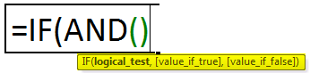
IF(AND()) — IF(AND(logical1, [logical2], …), value_if_true, [value_if_false]))
-
IF(OR()) — IF(OR(logical1, [logical2], …), value_if_true, [value_if_false]))
-
IF(NOT()) — IF(NOT(logical1), value_if_true, [value_if_false]))
|
Argument name |
Description |
|
|
logical_test (required) |
The condition you want to test. |
|
|
value_if_true (required) |
The value that you want returned if the result of logical_test is TRUE. |
|
|
value_if_false (optional) |
The value that you want returned if the result of logical_test is FALSE. |
|
Here are overviews of how to structure AND, OR and NOT functions individually. When you combine each one of them with an IF statement, they read like this:
-
AND – =IF(AND(Something is True, Something else is True), Value if True, Value if False)
-
OR – =IF(OR(Something is True, Something else is True), Value if True, Value if False)
-
NOT – =IF(NOT(Something is True), Value if True, Value if False)
Examples
Following are examples of some common nested IF(AND()), IF(OR()) and IF(NOT()) statements. The AND and OR functions can support up to 255 individual conditions, but it’s not good practice to use more than a few because complex, nested formulas can get very difficult to build, test and maintain. The NOT function only takes one condition.

Here are the formulas spelled out according to their logic:
|
Formula |
Description |
|---|---|
|
=IF(AND(A2>0,B2<100),TRUE, FALSE) |
IF A2 (25) is greater than 0, AND B2 (75) is less than 100, then return TRUE, otherwise return FALSE. In this case both conditions are true, so TRUE is returned. |
|
=IF(AND(A3=»Red»,B3=»Green»),TRUE,FALSE) |
If A3 (“Blue”) = “Red”, AND B3 (“Green”) equals “Green” then return TRUE, otherwise return FALSE. In this case only the first condition is true, so FALSE is returned. |
|
=IF(OR(A4>0,B4<50),TRUE, FALSE) |
IF A4 (25) is greater than 0, OR B4 (75) is less than 50, then return TRUE, otherwise return FALSE. In this case, only the first condition is TRUE, but since OR only requires one argument to be true the formula returns TRUE. |
|
=IF(OR(A5=»Red»,B5=»Green»),TRUE,FALSE) |
IF A5 (“Blue”) equals “Red”, OR B5 (“Green”) equals “Green” then return TRUE, otherwise return FALSE. In this case, the second argument is True, so the formula returns TRUE. |
|
=IF(NOT(A6>50),TRUE,FALSE) |
IF A6 (25) is NOT greater than 50, then return TRUE, otherwise return FALSE. In this case 25 is not greater than 50, so the formula returns TRUE. |
|
=IF(NOT(A7=»Red»),TRUE,FALSE) |
IF A7 (“Blue”) is NOT equal to “Red”, then return TRUE, otherwise return FALSE. |
Note that all of the examples have a closing parenthesis after their respective conditions are entered. The remaining True/False arguments are then left as part of the outer IF statement. You can also substitute Text or Numeric values for the TRUE/FALSE values to be returned in the examples.
Here are some examples of using AND, OR and NOT to evaluate dates.

Here are the formulas spelled out according to their logic:
|
Formula |
Description |
|---|---|
|
=IF(A2>B2,TRUE,FALSE) |
IF A2 is greater than B2, return TRUE, otherwise return FALSE. 03/12/14 is greater than 01/01/14, so the formula returns TRUE. |
|
=IF(AND(A3>B2,A3<C2),TRUE,FALSE) |
IF A3 is greater than B2 AND A3 is less than C2, return TRUE, otherwise return FALSE. In this case both arguments are true, so the formula returns TRUE. |
|
=IF(OR(A4>B2,A4<B2+60),TRUE,FALSE) |
IF A4 is greater than B2 OR A4 is less than B2 + 60, return TRUE, otherwise return FALSE. In this case the first argument is true, but the second is false. Since OR only needs one of the arguments to be true, the formula returns TRUE. If you use the Evaluate Formula Wizard from the Formula tab you’ll see how Excel evaluates the formula. |
|
=IF(NOT(A5>B2),TRUE,FALSE) |
IF A5 is not greater than B2, then return TRUE, otherwise return FALSE. In this case, A5 is greater than B2, so the formula returns FALSE. |

Using AND, OR and NOT with Conditional Formatting
You can also use AND, OR and NOT to set Conditional Formatting criteria with the formula option. When you do this you can omit the IF function and use AND, OR and NOT on their own.
From the Home tab, click Conditional Formatting > New Rule. Next, select the “Use a formula to determine which cells to format” option, enter your formula and apply the format of your choice.

Using the earlier Dates example, here is what the formulas would be.

|
Formula |
Description |
|---|---|
|
=A2>B2 |
If A2 is greater than B2, format the cell, otherwise do nothing. |
|
=AND(A3>B2,A3<C2) |
If A3 is greater than B2 AND A3 is less than C2, format the cell, otherwise do nothing. |
|
=OR(A4>B2,A4<B2+60) |
If A4 is greater than B2 OR A4 is less than B2 plus 60 (days), then format the cell, otherwise do nothing. |
|
=NOT(A5>B2) |
If A5 is NOT greater than B2, format the cell, otherwise do nothing. In this case A5 is greater than B2, so the result will return FALSE. If you were to change the formula to =NOT(B2>A5) it would return TRUE and the cell would be formatted. |
Note: A common error is to enter your formula into Conditional Formatting without the equals sign (=). If you do this you’ll see that the Conditional Formatting dialog will add the equals sign and quotes to the formula — =»OR(A4>B2,A4<B2+60)», so you’ll need to remove the quotes before the formula will respond properly.
Need more help?

See also
You can always ask an expert in the Excel Tech Community or get support in the Answers community.
Learn how to use nested functions in a formula
IF function
AND function
OR function
NOT function
Overview of formulas in Excel
How to avoid broken formulas
Detect errors in formulas
Keyboard shortcuts in Excel
Logical functions (reference)
Excel functions (alphabetical)
Excel functions (by category)
The IF function runs a logical test and returns one value for a TRUE result, and another value for a FALSE result. The result from IF can be a value, a cell reference, or even another formula. By combining the IF function with other logical functions like AND and OR, you can test more than one condition at a time.
Syntax
The generic syntax for the IF function looks like this:
=IF(logical_test,[value_if_true],[value_if_false])The first argument, logical_test, is typically an expression that returns either TRUE or FALSE. The second argument, value_if_true, is the value to return when logical_test is TRUE. The last argument, value_if_false, is the value to return when logical_test is FALSE. Both value_if_true and value_if_false are optional, but you must provide one or the other. For example, if cell A1 contains 80, then:
=IF(A1>75,TRUE) // returns TRUE
=IF(A1>75,"OK") // returns "OK"
=IF(A1>85,"OK") // returns FALSE
=IF(A1>75,10,0) // returns 10
=IF(A1>85,10,0) // returns 0
=IF(A1>75,"Yes","No") // returns "Yes"
=IF(A1>85,"Yes","No") // returns "No"
Notice that text values like «OK», «Yes», «No», etc. must be enclosed in double quotes («»). However, numeric values should not be enclosed in quotes.
Logical tests
The IF function supports logical operators (>,<,<>,=) when creating logical tests. Most commonly, the logical_test in IF is a complete logical expression that will evaluate to TRUE or FALSE. The table below shows some common examples:
| Goal | Logical test |
|---|---|
| If A1 is greater than 75 | A1>75 |
| If A1 equals 100 | A1=100 |
| If A1 is less than or equal to 100 | A1<=100 |
| If A1 equals «Red» | A1=»red» |
| If A1 is not equal to «Red» | A1<>»red» |
| If A1 is less than B1 | A1<B1 |
| If A1 is empty | A1=»» |
| If A1 is not empty | A1<>»» |
| If A1 is less than current date | A1<TODAY() |
Notice text values must be enclosed in double quotes («»), but numbers do not. The IF function does not support wildcards, but you can combine IF with COUNTIF to get basic wildcard functionality. To test for substrings in a cell, you can use the IF function with the SEARCH function.
Pass or Fail example
In the worksheet shown above, we want to assign either «Pass» or «Fail» based on a test score. A passing score is 70 or higher. The formula in D6, copied down, is:
=IF(C5>=70,"Pass","Fail")
Translation: If the value in C5 is greater than or equal to 70, return «Pass». Otherwise, return «Fail».
Note that the logical flow of this formula can be reversed. This formula returns the same result:
=IF(C5<70,"Fail","Pass")
Translation: If the value in C5 is less than 70, return «Fail». Otherwise, return «Pass».
Both formulas above, when copied down, will return correct results.
Note: If you are new to the idea of formula criteria, this article explains many examples.
Assign points based on color
In the worksheet below, we want to assign points based on the color in column B. If the color is «red», the result should be 100. If the color is «blue», the result should be 125. This requires that we use a formula based on two IF functions, one nested inside the other. The formula in C5, copied down, is:
=IF(B5="red",100,IF(B5="blue",125))
Translation: IF the value in B5 is «red», return 100. Else, if the value in B5 is «blue», return 125.

There are three things to notice in this example:
- The formula will return FALSE if the value in B5 is anything except «red» or «blue»
- The text values «red» and «blue» must be enclosed in double quotes («»)
- The IF function is not case-sensitive and will match «red», «Red», «RED», or «rEd».
This is a simple example of a nested IFs formula. See below for a more complex example.
Return another formula
The IF function can return another formula as a result. For example, the formula below will return A1*5% when A1 is less than 100, and A1*7% when A1 is greater than or equal to 100:
=IF(A1<100,A1*5%,A1*7%)
Nested IF statements
The IF function can be «nested». A «nested IF» refers to a formula where at least one IF function is nested inside another in order to test for more conditions and return more possible results. Each IF statement needs to be carefully «nested» inside another so that the logic is correct. For example, the following formula can be used to assign a grade rather than a pass / fail result:
=IF(C6<70,"F",IF(C6<75,"D",IF(C6<85,"C",IF(C6<95,"B","A"))))
Up to 64 IF functions can be nested. However, in general, you should consider other functions, like VLOOKUP or XLOOKUP for more complex scenarios, because they can handle more conditions in a more streamlined fashion. For a more details see this article on nested IFs.
Note: the newer IFS function is designed to handle multiple conditions without nesting. However, a lookup function like VLOOKUP or XLOOKUP is usually a better approach unless the logic for each condition is custom.
IF with AND, OR, NOT
The IF function can be combined with the AND function and the OR function. For example, to return «OK» when A1 is between 7 and 10, you can use a formula like this:
=IF(AND(A1>7,A1<10),"OK","")
Translation: if A1 is greater than 7 and less than 10, return «OK». Otherwise, return nothing («»).
To return B1+10 when A1 is «red» or «blue» you can use the OR function like this:
=IF(OR(A1="red",A1="blue"),B1+10,B1)
Translation: if A1 is red or blue, return B1+10, otherwise return B1.
=IF(NOT(A1="red"),B1+10,B1)
Translation: if A1 is NOT red, return B1+10, otherwise return B1.
IF cell contains specific text
Because the IF function does not support wildcards, it is not obvious how to configure IF to check for a specific substring in a cell. A common approach is to combine the ISNUMBER function and the SEARCH function to create a logical test like this:
=ISNUMBER(SEARCH(substring,A1)) // returns TRUE or FALSEFor example, to check for the substring «xyz» in cell A1, you can use a formula like this:
=IF(ISNUMBER(SEARCH("xyz",A1)),"Yes","No")Read a detailed explanation here.
More information
- Read more about nested IFs
- Learn how to use VLOOKUP instead of nested IFs (video)
- 50 Examples of formula criteria
Notes
- The IF function is not case-sensitive.
- To count values conditionally, use the COUNTIF or the COUNTIFS functions.
- To sum values conditionally, use the SUMIF or the SUMIFS functions.
- If any of the arguments to IF are supplied as arrays, the IF function will evaluate every element of the array.
IF function is undoubtedly one of the most important functions in excel. In general, IF statements give the desired intelligence to a program so that it can make decisions based on given criteria and, most importantly, decide the program flow.
In Microsoft Excel terminology, IF statements are also called «Excel IF-Then statements». IF function evaluates a boolean/logical expression and returns one value if the expression evaluates to ‘TRUE’ and another value if the expression evaluates to ‘FALSE’.
Definition of Excel IF Function
According to Microsoft Excel, IF function is defined as a formula which «checks whether a condition is met, returns one value if true and another value if false».
Syntax
Syntax of IF function in Excel is as follows:
=IF(logic_test, [value_if_true], [value_if_false])
'logic_test' (required argument) – Refers to the boolean expression or logical expression that needs to be evaluated.'value_if_true' (optional argument) – Refers to the value that will be returned by the IF function if the 'logic_test' evaluates to TRUE.'value_if_false' (optional argument) – Refers to the value that will be returned by the IF function if the 'logic_test' evaluates to FALSE.

Important Characteristics of IF Function in Excel
- To use the IF function, you need to provide the
'logic_test'or conditional statement mandatorily. - The arguments
'value_if_true'and'value_if_false'are optional, but you need to provide at least one of them. - The result of the IF statement can only be any one of the two given values (either it will be
'value_if_true'or'value_if_false'). Both values cannot be returned at the same time. - IF function throws a ‘#Name?’ error if the
'logic_test'or boolean expression you are trying to evaluate is invalid. - Nesting of IF statements is possible, but Excel only allows this to 64 levels. Nesting of IF statement means using one if statement within another.
Comparison Operators That Can Be Used With IF Statements
Following comparison operators can be used within the 'logic_test' argument of the IF function:
- = (equal to)
- <> (not equal to)
- < (less than)
- > (greater than)
- >= (greater than or equal to)
- <= (less than or equal to)
- Apart from these, you can also use any other function that returns a boolean result (either ‘true’ or ‘false’). For example – ISBLANK, ISERROR, ISEVEN, ISODD, etc
Now, let’s see some simple examples to use these comparison operators within the IF Function:
Simple Examples of Excel IF Statement
Now, let’s try to see a simple example of the Excel IF function:
Example 1: Using ‘equal to’ comparison operator within the IF function
In this example, we have a list of colors, and we aim to find the ‘Blue’ color. If we are able to find the ‘Blue’ color, then in the adjacent cell, we need to assign a ‘Yes’; otherwise, assign a ‘No’.

So, the formula would be:
=IF(A2="Blue", "No", "Yes")
This suggests that if the value present in cell A2 is ‘Blue’, then return a ‘Yes’; otherwise, return a ‘No’.
If we drag this formula down to all the rows, we will find that it returns ‘Yes’ for the cells with the value ‘Blue’ for all others; it would result in ‘No’.
Example 2: Using ‘not equal to’ comparison operator within the IF function.
Let’s take example 1, and understand how we can reverse the logic and use a ‘not equal to’ operator to construct the formula so that it still results in ‘Yes’ for ‘Blue’ color and ‘No’ for any other text.

So the formula would be:
=IF(A2<>"Blue", "No", "Yes")
This suggests that if the value at A2 is not equal to ‘Blue’, then return a ‘No’; otherwise, return a ‘Yes’.
When dragged down to all the below rows, this formula would find all the cells (from A2 to A8) where the value is not ‘Blue’ and marks a ‘No’ against them. Otherwise, it marks a ‘Yes’ in the adjacent cells.
Example 3: Using ‘less than’ operator within the IF function.
In this example, we have scores of some students, along with their names. We want to assign either «Pass» or «Fail» against each student in the result column.

Based on our criteria, the passing score is 50 or more.
For this, we can use the IF function as:
=IF(B2<50,"Fail","Pass")
This suggests that if the value at B2, i.e., 37, is less than 50, then return «Fail»; otherwise, return «Pass».
As 37 is less than 50 so the result will be «Fail».
We can drag the above-given formula for the rest of the cells below and the result would be correct.
Example 4: Using ‘greater than or equal to’ operator within the IF statement.
Let’s take example 3 and see how we can reverse the logic and use a ‘greater than or equal to’ operator to construct the formula so that it still results in ‘Pass’ for scores of 50 or more and ‘Fail’ for all the other scores.

For this, we can use the Excel IF function as:
=IF(B2>=50,"Pass","Fail")
This suggests that if the value at B2, i.e., 37 is greater than or equal to 50, then return «Pass»; otherwise, return «Fail».
As 37 not greater than or equal to 50 so the result will be «Fail».
When dragged down for the rest of the cells below, this formula would assign the correct result in the adjacent rows.
Example 5: Using ‘greater than’ operator within the IF statement.
In this example, we have a small online store that gives a discount to its customers based on the amount they spend. If a customer spends $50 or more, he is applicable for a 5% discount; otherwise, no discounts are offered.

To find whether a discount is offered or not, we can use the following excel formula:
=IF(B2>50,"5% Discount","No Discount")
This translates to – If the value at B2 cell is greater than 50, assign a text «5% Discount» otherwise, assign a text «No Discount» against the customer.
In the first case, as 23 is not greater than 50, the output will be «No Discount».
We can drag the above-given formula for the rest of the cells below are the result would be correct.
Example 6: Using ‘less than or equal to’ operator within the IF statement.
Let’s take example 5 and see how we can reverse the logic and use a ‘less than or equal to’ operator to construct the formula so that it still results in a ‘5% Discount’ for all customers whose total spend exceeds $50 and ‘No Discount’ for all the other customers.

For this, we can use the IF-then statement as:
=IF(B2<=50,"No Discount","5% Discount")
This means that if the value at B2, i.e., 23, is less than or equal to 50, then return «No Discount»; otherwise, return «5% Discount».
As 23 is less than or equal to 50 so the result will be «No Discount».
When dragged down for the rest of the cells below, this formula would assign the correct result in the adjacent rows.
Example 7: Using an Excel Logical Function within the IF formula in Excel.
In this example, let’s suppose we have a list of numbers, and we have to mark Even and Odd numbers. We can do this using the IF condition and the ISEVEN or ISODD inbuilt functions provided by Microsoft Excel.
ISEVEN function returns ‘true’ if the number passed to it is even; otherwise, it returns a ‘false’. Similarly, ISODD function return ‘true’ if the number passed to it is odd; otherwise, it returns a ‘false’.

For this, we can use the IF-then statement as:
=IF(ISEVEN(A2),"Even","Odd")
This means that – If the value at A2 cell is an even number, then the result would be «Even»; otherwise, the result would be «Odd».
Alternatively, the above logic can also be written using the ISODD function along with the IF statement as:
=IF(ISODD(A2),"Odd","Even")
This means that – If the value at A2 cell is an odd number, then the result would be «Odd»; otherwise, the result would be «Even».
Example 8: Using the Excel IF function to return another formula a result.
In this example, we have Employee Data from a company. The company comes up with a simple way to reward its loyal employees. They decide to give the employees an annual bonus based on the years spent by the employee within the organization.
Employees with experience of more than 5 years are given 10% of annual salary as a bonus whereas everyone else gets a 5% of annual salary as a bonus.

For this, the excel formula would be:
=IF(B2>5,C2*10%,C2*5%)
This means that – if the value at B2 (experience column) is greater than 5, then return a result by calculating 10% of C2 (annual salary column). However, if the logic test is evaluated to false, then return the result by calculating 5% of C2 (annual salary column)
Use Of AND & OR Functions or Logical Operators with Excel IF Statement
Excel IF Statement can also be used along with the other functions like AND, OR, NOT for analyzing complex logic. These functions (AND, OR & NOT) are called logical operators as they are used for connecting two or more logical expressions.
AND Function– AND function returns true when all the conditions inside the AND function evaluate to true. The syntax of AND Function in Excel is:
=AND(Logic1, Logic2, logic_n)
OR Function– OR function returns true when any one of the conditions inside the OR function evaluates to true. The syntax of OR Function in Excel is:
=OR(Logic1, Logic2, logic_n)
Example 9: Using the IF function along with AND Function.
In this example, we have Math and science test scores of some students, and we want to assign a ‘Pass’ or ‘Fail’ value against the students based on their scores.
Passing criteria: Students have to get more than 50 marks in Math and more than 70 marks in science to pass the test.

Based on the above conditions, the formula would be:
=IF(AND(B2>50,C2>70),"Pass","Fail")
The formula translates to – if the value at B2 (Math score) is greater than 50 and the value at C2 (Science Score) is greater than 70, then assign the value «Pass»; otherwise, assign the value «Fail».
Example 10: Using the IF function along with OR Function.
In this example, we have two test scores of some students, and we want to assign a ‘Pass’ or ‘Fail’ value against the students based on their scores.
Passing criteria: Students have to clear either one of the two tests with more than 50 marks.

Based on the above conditions, the formula would be:
=IF(OR(B2>50,C2>50),"Pass","Fail")
The formula translates to – if either the value at B2 (Test 1 score) is greater than 50, OR the value at C2 (Test 2 Score) is greater than 50, then assign the value «Pass»; otherwise, assign the value «Fail».
Recommended Reading: Excel NOT Function
Nested IF Statements
When used alone, IF formula can only result in two outcomes, i.e., True or False. But there are many cases when we want to test multiple outcomes with IF statement.
In such cases, nesting two or more IF Then statements one inside another can be convenient in writing formulas.
Syntax:
The syntax of the Nested IF Then statements is as follows:
=IF(condition_1,value_if_true_1,IF(condition_2,value_if_true_2,value_if_false_2))
'condition_1' – Refers to the first logical test or conditional expression that needs to be evaluated by the outer IF function.'value_if_true_1' – Refers to the value that will be returned by the outer IF function if the 'condition_1' evaluates to TRUE.'condition_2' – Refers to the second logical test or conditional expression that needs to be evaluated by the inner IF function.'value_if_true_2' – Refers to the value that will be returned by the inner IF function if the 'condition_2' evaluates to TRUE.'value_if_false_2' – Refers to the value that will be returned by the inner IF function if the 'condition_2' evaluates to FALSE.
The above syntax translates to this:
IF Condition1 = true THEN value_if_true1 'If Condition1 is true
ELSE IF Condition2 = true THEN value_if_true2 'Elseif Clause Condition2 is true
ELSE value_if_false2 'If both conditions are false
END IF 'End of IF Statement
As we can see, Nested formulas can quickly become complicated so, let’s try to understand how nesting of the IF statement works with an example.
Recommended Reading: VBA Select Case Statement
Example 11: Nested IF Statements
In this example, we have a list of countries and their average temperatures in degree Celsius for the month of January. Our goal is to categorize the country based on the temperature range as follows:
Criteria: Temperatures below 20 °C should be marked as «Below Room Temperature», temperatures between 20°C to 25°C should be classified as «Normal Room Temperature», whereas any temperature over 25°C should be marked as «Above Room Temperature».

Based on the above conditions, the formula would be:
=IF(B2<20,"Below Room Temperature",IF(AND(B2>=20,B2<=25),"Normal Room Temperature", "Above Room Temperature"))
The formula translates to – if the value at B2 is less than 20, then the text «Below Room Temperature» is returned from the outer IF block. However, if the value at B2 is greater than or equal to 20, then the inner IF block is evaluated.
Inside the inner IF block, the value at B2 is checked. If the value at B2 is greater than or equal to 20 and less than or equal to 25. Then the inner IF block returns the text «Normal Room Temperature».
However, if the condition inside the inner IF block also evaluates to ‘false’ that means the value at B2 is greater than 25, so the result will be «Above Room Temperature».
Recommended Reading: SWITCH Function in Excel
Partial Matching or Wildcards with IF Function
Although IF function itself doesn’t accept any wildcard characters like (* or ?) while performing the logic test, thankfully, there are ways to perform partial matching and wildcard searches with the IF function.
To perform partial matching inside the IF function, we can use the FIND (case sensitive) or SEARCH (case insensitive) functions.
Let’s have a look at this with some examples.
Example 12: Using FIND and SEARCH functions inside the IF statement
In this example, we have a list of customers, and we need to find all the customers whose last name is «Flynn». If the customer name contains the text «Flynn», then we need to assign a text «Found» against their names. Otherwise, we need to assign a text «Not Found».

For this, we can make use of the FIND function within the IF function as:
=IF(ISNUMBER(FIND("Flynn",A2)),"Found","Not Found")
Using the FIND function, we perform a case-sensitive search of the text «Flynn» within the customer name column. If the FIND function is able to find the text «Flynn», it returns a number signifying the position where it found the text.
If the number returned by the FIND function is valid, the ISNUMBER Function returns a value true. Else, it returns false. Based on the ISNUMBER function’s output, the logic test is performed and the appropriate value «Found» or «Not Found» is assigned.
Note: It should be noted that the FIND function performs a case-sensitive search.
This means in the above example if the customer name is entered in lower case (like «sean flynn» then the above function would return not found against them.
To perform a case-insensitive search, we can replace the find function with the search function, and the rest of the formula would be the same.
=IF(ISNUMBER(SEARCH("Flynn",A2)),"Found","Not Found")
Example 13: Using SEARCH function inside the Excel IF formula with wildcard operators
In this example, we have the same customer list from example 12, and we need to find all the customers whose name contains «M». If the customer name contains the alphabet «M», we need to assign a text «M Found» against their names. Otherwise, we need to assign a text «M Not Found».

For this, we can use the SEARCH function with a wildcard ‘*’ operator inside the IF function as:
=IF(ISNUMBER(SEARCH("M*",A2)),"M Found","M Not Found")
For more details on Search Function and wildcard, operators check out this article – Search Function In Excel
Some Practical Examples of using the IF function
Now, let’s have a look at some more practical examples of the Excel IF Function.
Example 14: Using Excel IF function with dates.
In this example, we have a task list along with the task due dates. Our goal is to show results based on the task due date.
If the task due date was in the past, we need to show «Was due {1,2,3..} day(s) back», if the task due date is today’s date, we need to show «Today» and similarly, if the task due date is in the future then we need to show «Due in {1,2,3..} day(s)»

In Microsoft Excel, we can do this with the help of the IF-then statement and TODAY function, as shown below:
=IF(B2=TODAY(),"Today", IF(B2>TODAY(),CONCAT("Due in ",B2-TODAY()," day(s)"), CONCAT("Was due ",TODAY()-B2," day(s) back")))
This means that – compare the date present in cell B2 if the date is equal to today’s date show the text «Today». If the date in cell B2 is not equal to today’s date, then the inner IF block checks if the date in B2 is greater than today’s date. If the date in cell B2 is greater than today’s date, that means the date is in the future, so show the text «Due in {1,2,3…} days».
However, if the date in cell B2 is not greater than today’s date, that means the date was in the past; in such a case, show the text «Was due {1,2,3..} day(s) back».
You can also go a step further and apply conditional formatting on the range and highlight all the cells with the text «Today!». This will help you to clearly see
Example 15: Use an IF function-based formula to find blank cells in excel.
In this example, we will use the IF function to find the blank cells in Microsoft Excel. We have a list of customers, and in between the list, some of the cells are blank. We aim to find the blank cells and add the text «blank call found!» against them.

We can do this with the help of the IF function along with the ISBLANK function. The ISBLANK function returns a true if the cell reference passed to it is blank. Otherwise, the ISBLANK function returns false.
Let’s see the formula –
=IF(ISBLANK(A2), "Blank cell found!"," ")
This means that – If the cell at A2 is blank, then the resultant text should be «Blank cell found!», however, if the cell at A2 is not blank, then don’t show any text.
Example 16: Use the Excel IF statement to show symbolic results (instead of textual results).
In this example, we have a list of sales employees of a company along with the number of products sold by the employees in the current month. We want to show an upward arrow symbol (↑) if the employee has done more than 50 sales and a downward arrow symbol (↓) if the employee has made less than 50 sales.

To do this, we can use the formula:
=IF(B2>50,$G$6,$G$8)
This implies – If the value at B2 is greater than 50, then, as a result, show the content in cell G6 (cell containing upward arrow) and otherwise show the content at G8 (cell containing downward arrow)
If you wonder about the ‘$’ signs used in the formula, you can check out this post – Excel Absolute References. These ‘$’ symbols are used for making excel cell references absolute.
Recommended Reading: CHOOSE Function in Excel
IFS Function In Excel:
IFS Function in Microsoft Excel is a great alternative to nested IF Statements. It is very similar to a switch statement. The IFS function evaluates multiple conditions passed to it and returns the value corresponding to the first condition that evaluates to true.
IFS function is a lot simple to write and read than nested IF statements. IFS function is available in Office 2019 and higher versions.
Syntax for IFS function:
=IFS (test1, value1, [test2, value2], ...)
'test1' (required argument) – Refers to the first logical test that needs to be evaluated.
'value1' (required argument) – Refers to the result to be returned when 'test1'evaluates to TRUE.
'test2' (optional argument) – Refers to the second logical test that needs to be evaluated
'value2' (optional argument) – Refers to the result to be returned when 'test2'evaluates to TRUE.
Example 17: Using IFS function in Excel
In this example, we have a list of students, along with their scores, and we need to assign a grade to the students based on the scores.
The grading criteria is as follows – Grade A for a score of 90 or more, Grade B for a score between 80 to 89.99, Grade C for a score between 70 to 79.99, Grade D for a score between 60 to 69.99, Grade E for a score between 60 to 59.99, Grade F for a score lower than 50.

Let’s see how easily write such a complicated formula with the IFS function:
=IFS(B2 >= 90,"A",B2 >= 80,"B",B2 >= 70,"C",B2 >= 60,"D",B2 >= 50,"E",B2 < 50,"F")
This implies that – If B2 is greater than or equal to 90, return A. Else if B2 is greater than or equal to 80, return B. Else if B2 is greater than or equal to 70, return C. Else if B2 is greater than or equal to 60, return D. Else if B2 is greater than or equal to 50, return E. Else if B2 is less than 50, return F.
If you would try to write the same formula using nested IF statements, see how long and complicated it becomes:
=IF(B2 >= 90,"A",IF(B2 >= 80, "B",IF(B2 >= 70, "C",IF(B2 >= 60, "D",IF(B2 >= 50, "E",IF(B2 < 50, "F"))))))
So, this was all about the IF function in excel. If you want to learn more about IF function, I would recommend you to go through this article – VBA IF Statement With Examples
Функция ЕСЛИ в Excel — это отличный инструмент для проверки условий на ИСТИНУ или ЛОЖЬ. Если значения ваших расчетов равны заданным параметрам функции как ИСТИНА, то она возвращает одно значение, если ЛОЖЬ, то другое.
Содержание
- Что возвращает функция
- Синтаксис
- Аргументы функции
- Дополнительная информация
- Функция Если в Excel примеры с несколькими условиями
- Пример 1. Проверяем простое числовое условие с помощью функции IF (ЕСЛИ)
- Пример 2. Использование вложенной функции IF (ЕСЛИ) для проверки условия выражения
- Пример 3. Вычисляем сумму комиссии с продаж с помощью функции IF (ЕСЛИ) в Excel
- Пример 4. Используем логические операторы (AND/OR) (И/ИЛИ) в функции IF (ЕСЛИ) в Excel
- Пример 5. Преобразуем ошибки в значения “0” с помощью функции IF (ЕСЛИ)
Что возвращает функция
Заданное вами значение при выполнении двух условий ИСТИНА или ЛОЖЬ.
Синтаксис
=IF(logical_test, [value_if_true], [value_if_false]) — английская версия
=ЕСЛИ(лог_выражение; [значение_если_истина]; [значение_если_ложь]) — русская версия
Аргументы функции
- logical_test (лог_выражение) — это условие, которое вы хотите протестировать. Этот аргумент функции должен быть логичным и определяемым как ЛОЖЬ или ИСТИНА. Аргументом может быть как статичное значение, так и результат функции, вычисления;
- [value_if_true] ([значение_если_истина]) — (не обязательно) — это то значение, которое возвращает функция. Оно будет отображено в случае, если значение которое вы тестируете соответствует условию ИСТИНА;
- [value_if_false] ([значение_если_ложь]) — (не обязательно) — это то значение, которое возвращает функция. Оно будет отображено в случае, если условие, которое вы тестируете соответствует условию ЛОЖЬ.
Дополнительная информация
- В функции ЕСЛИ может быть протестировано 64 условий за один раз;
- Если какой-либо из аргументов функции является массивом — оценивается каждый элемент массива;
- Если вы не укажете условие аргумента FALSE (ЛОЖЬ) value_if_false (значение_если_ложь) в функции, т.е. после аргумента value_if_true (значение_если_истина) есть только запятая (точка с запятой), функция вернет значение “0”, если результат вычисления функции будет равен FALSE (ЛОЖЬ).
На примере ниже, формула =IF(A1> 20,”Разрешить”) или =ЕСЛИ(A1>20;»Разрешить») , где value_if_false (значение_если_ложь) не указано, однако аргумент value_if_true (значение_если_истина) по-прежнему следует через запятую. Функция вернет “0” всякий раз, когда проверяемое условие не будет соответствовать условиям TRUE (ИСТИНА).
 |
| - Если вы не укажете условие аргумента TRUE(ИСТИНА) (value_if_true (значение_если_истина)) в функции, т.е. условие указано только для аргумента value_if_false (значение_если_ложь), то формула вернет значение “0”, если результат вычисления функции будет равен TRUE (ИСТИНА);
На примере ниже формула равна =IF (A1>20;«Отказать») или =ЕСЛИ(A1>20;»Отказать»), где аргумент value_if_true (значение_если_истина) не указан, формула будет возвращать “0” всякий раз, когда условие соответствует TRUE (ИСТИНА).

Функция Если в Excel примеры с несколькими условиями
Пример 1. Проверяем простое числовое условие с помощью функции IF (ЕСЛИ)
При использовании функции ЕСЛИ в Excel, вы можете использовать различные операторы для проверки состояния. Вот список операторов, которые вы можете использовать:
Ниже приведен простой пример использования функции при расчете оценок студентов. Если сумма баллов больше или равна «35», то формула возвращает “Сдал”, иначе возвращается “Не сдал”.
Пример 2. Использование вложенной функции IF (ЕСЛИ) для проверки условия выражения
Функция может принимать до 64 условий одновременно. Несмотря на то, что создавать длинные вложенные функции нецелесообразно, то в редких случаях вы можете создать формулу, которая множество условий последовательно.
В приведенном ниже примере мы проверяем два условия.
- Первое условие проверяет, сумму баллов не меньше ли она чем 35 баллов. Если это ИСТИНА, то функция вернет “Не сдал”;
- В случае, если первое условие — ЛОЖЬ, и сумма баллов больше 35, то функция проверяет второе условие. В случае если сумма баллов больше или равна 75. Если это правда, то функция возвращает значение “Отлично”, в других случаях функция возвращает “Сдал”.
Пример 3. Вычисляем сумму комиссии с продаж с помощью функции IF (ЕСЛИ) в Excel
Функция позволяет выполнять вычисления с числами. Хороший пример использования — расчет комиссии продаж для торгового представителя.
В приведенном ниже примере, торговый представитель по продажам:
- не получает комиссионных, если объем продаж меньше 50 тыс;
- получает комиссию в размере 2%, если продажи между 50-100 тыс
- получает 4% комиссионных, если объем продаж превышает 100 тыс.
Рассчитать размер комиссионных для торгового агента можно по следующей формуле:
=IF(B2<50,0,IF(B2<100,B2*2%,B2*4%)) — английская версия
=ЕСЛИ(B2<50;0;ЕСЛИ(B2<100;B2*2%;B2*4%)) — русская версия
В формуле, использованной в примере выше, вычисление суммы комиссионных выполняется в самой функции ЕСЛИ. Если объем продаж находится между 50-100K, то формула возвращает B2 * 2%, что составляет 2% комиссии в зависимости от объема продажи.
Больше лайфхаков в нашем Telegram Подписаться
Пример 4. Используем логические операторы (AND/OR) (И/ИЛИ) в функции IF (ЕСЛИ) в Excel
Вы можете использовать логические операторы (AND/OR) (И/ИЛИ) внутри функции для одновременного тестирования нескольких условий.
Например, предположим, что вы должны выбрать студентов для стипендий, основываясь на оценках и посещаемости. В приведенном ниже примере учащийся имеет право на участие только в том случае, если он набрал более 80 баллов и имеет посещаемость более 80%.
Вы можете использовать функцию AND (И) вместе с функцией IF (ЕСЛИ), чтобы сначала проверить, выполняются ли оба эти условия или нет. Если условия соблюдены, функция возвращает “Имеет право”, в противном случае она возвращает “Не имеет право”.
Формула для этого расчета:
=IF(AND(B2>80,C2>80%),”Да”,”Нет”) — английская версия
=ЕСЛИ(И(B2>80;C2>80%);»Да»;»Нет») — русская версия
Пример 5. Преобразуем ошибки в значения “0” с помощью функции IF (ЕСЛИ)
С помощью этой функции вы также можете убирать ячейки содержащие ошибки. Вы можете преобразовать значения ошибок в пробелы или нули или любое другое значение.
Формула для преобразования ошибок в ячейках следующая:
=IF(ISERROR(A1),0,A1) — английская версия
=ЕСЛИ(ЕОШИБКА(A1);0;A1) — русская версия
Формула возвращает “0”, в случае если в ячейке есть ошибка, иначе она возвращает значение ячейки.
ПРИМЕЧАНИЕ. Если вы используете Excel 2007 или версии после него, вы также можете использовать функцию IFERROR для этого.
Точно так же вы можете обрабатывать пустые ячейки. В случае пустых ячеек используйте функцию ISBLANK, на примере ниже:
=IF(ISBLANK(A1),0,A1) — английская версия
=ЕСЛИ(ЕПУСТО(A1);0;A1) — русская версия
IF AND Excel Formula
The IF AND excel formula is the combination of two different logical functions often nested together that enables the user to evaluate multiple conditions using AND functions. Based on the output of the AND function, the IF function returns either the “true” or “false” value, respectively.
- The IF formula in ExcelIF function in Excel evaluates whether a given condition is met and returns a value depending on whether the result is “true” or “false”. It is a conditional function of Excel, which returns the result based on the fulfillment or non-fulfillment of the given criteria.
read more is used to test and compare the conditions expressed with the expected value. It is used to test a single criterion. - The logical AND formula is used to test multiple criteria. It returns “true” if all the conditions mentioned are satisfied, or else returns “false.” It tests more than one criterion and accordingly returns an output. It can also be used along with the IF formula to return the desired result.
Table of contents
- IF AND Excel Formula
- Syntax
- How to Use IF AND Excel Statement?
- Example #1
- Example #2
- Example #3
- The Characteristics of IF AND function
- Frequently Asked Questions
- Recommended Articles
Syntax
The IF AND formula can be applied as follows:
“=IF(AND (Condition 1,Condition 2,…),Value _if _True,Value _if _False)”
You are free to use this image on your website, templates, etc, Please provide us with an attribution linkArticle Link to be Hyperlinked
For eg:
Source: IF AND in Excel (wallstreetmojo.com)
How to Use IF AND Excel Statement?
You can download this IF AND Formula Excel Template here – IF AND Formula Excel Template
Let us understand the usage of the IF AND formula with the help of some examples mentioned below:
Example #1
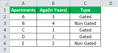
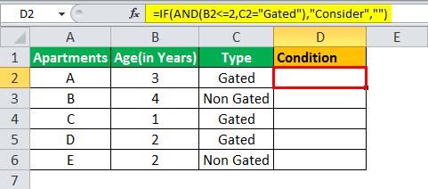
The table given below provides a list of apartments along with their age (in years) and type of society. Now we need to perform a comparative analysis for the apartments based on the age of the building and the type of society.
Here, we use the combination of less than equal (<=) to operator and the equal to (=) text functions in the condition to be demonstrated for IF AND function.
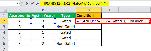
- The IF AND formula used to perform the analysis is stated as follows:
“=IF(AND(B2<=2,C2=“Gated”),“Consider”, “”)”
- The succeeding image shows the IF AND condition applied to perform the evaluation.
- Press “Enter” to get the answer.
- Drag the formula to find the results for all the apartments.
The results in the cell D of the above table shows that the IF AND formula will be performing one among the following:
- If both the arguments entered in the AND function is “true,” then the IF function will return that apartment to be “Consider.”
- If either of the arguments in the AND functionThe AND function in Excel is classified as a logical function; it returns TRUE if the specified conditions are met, otherwise it returns FALSE.read more is “false” or both the arguments entered are “false,” then the IF function will return a blank string.
The IF AND formula can also perform calculations based on whether the AND function returns “true” or “false,” apart from returning only the predefined text strings.
We will understand this concept with the help of the below-mentioned example.
Example #2
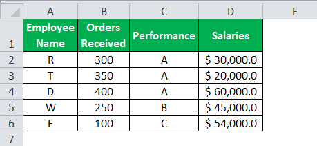
The given data tableA data table in excel is a type of what-if analysis tool that allows you to compare variables and see how they impact the result and overall data. It can be found under the data tab in the what-if analysis section.read more has the list of employee name along with their orders received, performance, and salaries. Calculate the employee hike (or bonus) based on two parameters–the number of orders received and performance.
The criteria to calculate the bonus is as follows.
- The number of orders received is greater than or equal to 200, and the performance is equal to “A.”
- The IF AND formula will be,
“=IF(AND(B2>=200,C2= “A”),D2*10%,D2*5%)”
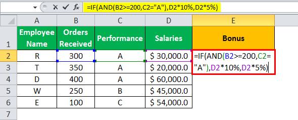
- Press “Enter” to get the final output. The bonus appears in cell E2.
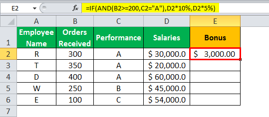
- Drag the formula to find the bonus of all employees.
Based on these results, the IF formula does the following evaluation:
- If both the conditions are satisfied, the AND function returns “true,” then the bonus received is calculated as salary multiplied by 10%.
- If either one or both the conditions are found to be “false” by the AND function, then the bonus is calculated as salary multiplied by 5%.
Examples 1 and 2 have only two criteria to test and evaluate. Using multiple arguments or conditions to test them for “true” or “false” is also allowed.
Example #3
Let us evaluate multiple criteria and use AND function.
A table with five stocks and their parameter details including financial ratiosFinancial ratios are indications of a company’s financial performance. There are several forms of financial ratios that indicate the company’s results, financial risks, and operational efficiency, such as the liquidity ratio, asset turnover ratio, operating profitability ratios, business risk ratios, financial risk ratio, stability ratios, and so on.read more, such as ROCEReturn on Capital Employed (ROCE) is a metric that analyses how effectively a company uses its capital and, as a result, indicates long-term profitability. ROCE=EBIT/Capital Employed.read more, ROEReturn on Equity (ROE) represents financial performance of a company. It is calculated as the net income divided by the shareholders equity. ROE signifies the efficiency in which the company is using assets to make profit.read more, Debt to equityThe debt to equity ratio is a representation of the company’s capital structure that determines the proportion of external liabilities to the shareholders’ equity. It helps the investors determine the organization’s leverage position and risk level. read more, and PE ratioThe price to earnings (PE) ratio measures the relative value of the corporate stocks, i.e., whether it is undervalued or overvalued. It is calculated as the proportion of the current price per share to the earnings per share. read more is provided (shown in the below table). Using this data lets us test the condition to invest in suitable stocks. That is, using the parameters, let us analyze the stocks to derive the best investment horizonThe term «investment horizon» refers to the amount of time an investor is expected to hold an investment portfolio or a security before selling it. Depending on the need for funds and risk appetite, the investor may invest for a few days or hours to a few years or decades.read more, which is important for growth.
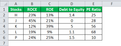
The following syntax is used where the conditions are applied to arrive at the result (shown in the below table).
“=IF(AND(B2>18%,C2>20%,D2<2,E2<30%),“Invest”,“”)”

- Press “Enter” to get the final output (Investment Criteria) of the above formula.

- Drag the formula to find the Investment Criteria.
In the above data table, the AND function tests for the parameters using the operators. The resulting output generated by the IF formula is as follows:
- If all the four criteria mentioned in the AND function are tested and satisfied, then the IF function returns the “Invest” text string.
- If either one or more among the four conditions or all the four conditions fail to satisfy the AND function, then the IF function returns empty strings (“”).
The Characteristics of IF AND function
- The IF AND function does not differentiate between case-insensitive texts.
- The AND function can be used to evaluate up to 255 conditions for “true” or “false,” and the total formula length does not exceed 8192 characters.
- Text values or blank cells are given as an argument to test the conditions in AND function.
- The AND formula will return “#VALUE!” if there is no logical output found while evaluating the conditions.
- IF AND excel statement is a combination of two logical functions that tests and evaluates multiple conditions.
- The output of the AND function is based on, whether the IF function will return the value “true” or “false,” respectively.
- IF function is used to test a single criterion whereas, the AND function is used to test multiple criteria.
- The syntax of the IF AND formula is:
“=IF(AND (Condition 1,Condition 2,…),Value _if _True,Value _if _False)”
- The IF AND formula also performs a calculation based on whether the AND function is “true” or “false” apart from returning only the predefined text strings.
Frequently Asked Questions
1. How to use IF AND function in Excel?
The IF AND excel statement is the two logical functions often nested together.
Syntax:
“=IF(AND(Condition1,Condition2, value_if_true,vaue_if_false)”
The IF formula is used to test and compare the conditions expressed, along with the expected value. It provides the desired result if the condition is either “true” or “false.”
The AND formula is used to test multiple criteria. It returns “true” if all the given conditions are satisfied, or else returns “false.”
2. What is the IF AND function in Excel?
IF AND formula is applied as the combination of the two logical functions that enable the user to evaluate the multiple conditions. Based on the output of the AND function, the IF function returns the output “true” or “false.”
3. How to combine IF and AND functions in Excel?
To combine IF and AND functions, you need to replace the “condition_test” argument in the IF function with AND function.
“=IF(condition_test, value_if_true,vaue_if_false)”
“=IF(AND(Condition1,Condition2, value_if_true,vaue_if_false)”
In AND function we can use multiple conditions.
Recommended Articles
This has been a guide to IF AND function in Excel. Here we discuss how to use IF Formula combined with AND function along with examples and downloadable templates. You may also look at these useful functions in Excel –
- IF EXCEL FunctionIF function in Excel evaluates whether a given condition is met and returns a value depending on whether the result is “true” or “false”. It is a conditional function of Excel, which returns the result based on the fulfillment or non-fulfillment of the given criteria.
read more - Average IF Function
- SUMIF with Multiple CriteriaThe SUMIF (SUM+IF) with multiple criteria sums the cell values based on the conditions provided. The criteria are based on dates, numbers, and text. The SUMIF function works with a single criterion, while the SUMIFS function works with multiple criteria in excel.read more
- Nested If ConditionIn Excel, nested if function means using another logical or conditional function with the if function to test multiple conditions. For example, if there are two conditions to be tested, we can use the logical functions AND or OR depending on the situation, or we can use the other conditional functions to test even more ifs inside a single if.read more
The logical IF statement in Excel is used for the recording of certain conditions. It compares the number and / or text, function, etc. of the formula when the values correspond to the set parameters, and then there is one record, when do not respond — another.
Logic functions — it is a very simple and effective tool that is often used in practice. Let us consider it in details by examples.
The syntax of the function «IF» with one condition
The operation syntax in Excel is the structure of the functions necessary for its operation data.
=IF(boolean;value_if_TRUE;value_if_FALSE)
Let us consider the function syntax:
- Boolean – what the operator checks (text or numeric data cell).
- Value_if_TRUE – what will appear in the cell when the text or numbers correspond to a predetermined condition (true).
- Value_if_FALSE – what appears in the box when the text or the number does not meet the predetermined condition (false).
Example:

Logical IF functions.
The operator checks the A1 cell and compares it to 20. This is a «Boolean». When the contents of the column is more than 20, there is a true legend «greater 20». In the other case it’s «less or equal 20».
Attention! The words in the formula need to be quoted. For Excel to understand that you want to display text values.
Here is one more example. To gain admission to the exam, a group of students must successfully pass a test. The results are listed in a table with columns: a list of students, a credit, an exam.

The statement IF should check not the digital data type but the text. Therefore, we prescribed in the formula В2= «done» We take the quotes for the program to recognize the text correctly.
The function IF in Excel with multiple conditions
Usually one condition for the logic function is not enough. If you need to consider several options for decision-making, spread operators’ IF into each other. Thus, we get several functions IF in Excel.
The syntax is as follows:
Here the operator checks the two parameters. If the first condition is true, the formula returns the first argument is the truth. False — the operator checks the second condition.
Examples of a few conditions of the function IF in Excel:

It’s a table for the analysis of the progress. The student received 5 points:
- А – excellent;
- В – above average or superior work;
- C – satisfactory;
- D – a passing grade;
- E – completely unsatisfactory.
IF statement checks two conditions: the equality of value in the cells.

In this example, we have added a third condition, which implies the presence of another report card and «twos». The principle of the operator is the same.
Enhanced functionality with the help of the operators «AND» and «OR»
When you need to check out a few of the true conditions you use the function И. The point is: IF A = 1 AND A = 2 THEN meaning в ELSE meaning с.
OR function checks the condition 1 or condition 2. As soon as at least one condition is true, the result is true. The point is: IF A = 1 OR A = 2 THEN value B ELSE value C.
Functions AND & OR can check up to 30 conditions.
An example of using the operator AND:

It’s the example of using the logical operator OR.

How to compare data in two tables
Users often need to compare the two spreadsheets in an Excel to match. Examples of the «life»: compare the prices of goods in different bringing, to compare balances (accounting reports) in a few months, the progress of pupils (students) of different classes, in different quarters, etc.
To compare the two tables in Excel, you can use the COUNTIFS statement. Consider the order of application functions.
For example, consider the two tables with the specifications of various food processors. We planned allocation of color differences. This problem in Excel solves the conditional formatting.
Baseline data (tables, which will work with):

Select the first table. Conditional Formatting — create a rule — use a formula to determine the formatted cells:

In the formula bar write: = COUNTIFS (comparable range; first cell of first table)=0. Comparing range is in the second table.
To drive the formula into the range, just select it first cell and the last. «= 0» means the search for the exact command (not approximate) values.
Choose the format and establish what changes in the cell formula in compliance. It’s better to do a color fill.
Select the second table. Conditional Formatting — create a rule — use the formula. Use the same operator (COUNTIFS). For the second table formula:
Download all examples in Excel

Now it is easy to compare the characteristics of the data in the table.
Things will not always be the way we want them to be. The unexpected can happen. For example, let’s say you have to divide numbers. Trying to divide any number by zero (0) gives an error. Logical functions come in handy such cases. In this tutorial, we are going to cover the following topics.
In this tutorial, we are going to cover the following topics.
- What is a Logical Function?
- IF function example
- Excel Logic functions explained
- Nested IF functions
What is a Logical Function?
It is a feature that allows us to introduce decision-making when executing formulas and functions. Functions are used to;
- Check if a condition is true or false
- Combine multiple conditions together
What is a condition and why does it matter?
A condition is an expression that either evaluates to true or false. The expression could be a function that determines if the value entered in a cell is of numeric or text data type, if a value is greater than, equal to or less than a specified value, etc.
IF Function example
We will work with the home supplies budget from this tutorial. We will use the IF function to determine if an item is expensive or not. We will assume that items with a value greater than 6,000 are expensive. Those that are less than 6,000 are less expensive. The following image shows us the dataset that we will work with.
 and conditions in Excel")
- Put the cursor focus in cell F4
- Enter the following formula that uses the IF function
=IF(E4<6000,”Yes”,”No”)
HERE,
- “=IF(…)” calls the IF functions
- “E4<6000” is the condition that the IF function evaluates. It checks the value of cell address E4 (subtotal) is less than 6,000
- “Yes” this is the value that the function will display if the value of E4 is less than 6,000
-
“No” this is the value that the function will display if the value of E4 is greater than 6,000
When you are done press the enter key
You will get the following results
 and conditions in Excel")
Excel Logic functions explained
The following table shows all of the logical functions in Excel
| S/N | FUNCTION | CATEGORY | DESCRIPTION | USAGE |
|---|---|---|---|---|
| 01 | AND | Logical | Checks multiple conditions and returns true if they all the conditions evaluate to true. | =AND(1 > 0,ISNUMBER(1)) The above function returns TRUE because both Condition is True. |
| 02 | FALSE | Logical | Returns the logical value FALSE. It is used to compare the results of a condition or function that either returns true or false | FALSE() |
| 03 | IF | Logical |
Verifies whether a condition is met or not. If the condition is met, it returns true. If the condition is not met, it returns false. =IF(logical_test,[value_if_true],[value_if_false]) |
=IF(ISNUMBER(22),”Yes”, “No”) 22 is Number so that it return Yes. |
| 04 | IFERROR | Logical | Returns the expression value if no error occurs. If an error occurs, it returns the error value | =IFERROR(5/0,”Divide by zero error”) |
| 05 | IFNA | Logical | Returns value if #N/A error does not occur. If #N/A error occurs, it returns NA value. #N/A error means a value if not available to a formula or function. |
=IFNA(D6*E6,0) N.B the above formula returns zero if both or either D6 or E6 is/are empty |
| 06 | NOT | Logical | Returns true if the condition is false and returns false if condition is true |
=NOT(ISTEXT(0)) N.B. the above function returns true. This is because ISTEXT(0) returns false and NOT function converts false to TRUE |
| 07 | OR | Logical | Used when evaluating multiple conditions. Returns true if any or all of the conditions are true. Returns false if all of the conditions are false |
=OR(D8=”admin”,E8=”cashier”) N.B. the above function returns true if either or both D8 and E8 admin or cashier |
| 08 | TRUE | Logical | Returns the logical value TRUE. It is used to compare the results of a condition or function that either returns true or false | TRUE() |
A nested IF function is an IF function within another IF function. Nested if statements come in handy when we have to work with more than two conditions. Let’s say we want to develop a simple program that checks the day of the week. If the day is Saturday we want to display “party well”, if it’s Sunday we want to display “time to rest”, and if it’s any day from Monday to Friday we want to display, remember to complete your to do list.
A nested if function can help us to implement the above example. The following flowchart shows how the nested IF function will be implemented.
 and conditions in Excel")
The formula for the above flowchart is as follows
=IF(B1=”Sunday”,”time to rest”,IF(B1=”Saturday”,”party well”,”to do list”))
HERE,
- “=IF(….)” is the main if function
- “=IF(…,IF(….))” the second IF function is the nested one. It provides further evaluation if the main IF function returned false.
Practical example
 and conditions in Excel")
Create a new workbook and enter the data as shown below
 and conditions in Excel")
- Enter the following formula
=IF(B1=”Sunday”,”time to rest”,IF(B1=”Saturday”,”party well”,”to do list”))
- Enter Saturday in cell address B1
- You will get the following results
 and conditions in Excel")
Download the Excel file used in Tutorial
Summary
Logical functions are used to introduce decision-making when evaluating formulas and functions in Excel.
Как использовать функцию IF
Функция IF — это основная логическая функция в Excel, и поэтому она должна быть понятна первой. Он появится много раз на протяжении всей этой статьи.
Давайте посмотрим на структуру функции IF, а затем посмотрим несколько примеров ее использования.
Функция IF принимает 3 бита информации:
= IF (логический_тест, [value_if_true], [value_if_false])
- логический_тест: это условие для функции для проверки.
- value_if_true: действие, которое выполняется, если условие выполнено или является истинным.
- value_if_false: действие, которое нужно выполнить, если условие не выполнено или имеет значение false.
Операторы сравнения для использования с логическими функциями
При выполнении логического теста со значениями ячеек вы должны быть знакомы с операторами сравнения. Вы можете увидеть их в таблице ниже.

Теперь давайте посмотрим на некоторые примеры в действии.
Пример функции IF 1: текстовые значения
В этом примере мы хотим проверить, равна ли ячейка определенной фразе. Функция IF не учитывает регистр, поэтому не учитывает прописные и строчные буквы.
Следующая формула используется в столбце C для отображения «Нет», если столбец B содержит текст «Завершено» и «Да», если он содержит что-либо еще.
= ЕСЛИ (B2 = "Завершено", "Нет", "Да")

Хотя функция IF не чувствительна к регистру, текст должен точно соответствовать.
Пример функции IF 2: Числовые значения
Функция IF также отлично подходит для сравнения числовых значений.
В приведенной ниже формуле мы проверяем, содержит ли ячейка B2 число, большее или равное 75. Если это так, то мы отображаем слово «Pass», а если не слово «Fail».
= ЕСЛИ (В2> = 75, "Проход", "Сбой")

Функция IF — это намного больше, чем просто отображение разного текста в результате теста. Мы также можем использовать его для запуска различных расчетов.
В этом примере мы хотим предоставить скидку 10%, если клиент тратит определенную сумму денег. Мы будем использовать £ 3000 в качестве примера.
= ЕСЛИ (В2> = 3000, В2 * 90%, В2)

Часть формулы B2 * 90% позволяет вычесть 10% из значения в ячейке B2. Есть много способов сделать это.
Важно то, что вы можете использовать любую формулу в разделах value_if_true или value_if_false . И запускать различные формулы, зависящие от значений других ячеек, — очень мощный навык.
Пример функции IF 3: значения даты
В этом третьем примере мы используем функцию IF для отслеживания списка сроков исполнения. Мы хотим отобразить слово «Просрочено», если дата в столбце B уже в прошлом. Но если дата наступит в будущем, рассчитайте количество дней до даты исполнения.
Приведенная ниже формула используется в столбце C. Мы проверяем, меньше ли срок оплаты в ячейке B2, чем сегодняшний день (функция TODAY возвращает сегодняшнюю дату с часов компьютера).
= ЕСЛИ (В2 <СЕГОДНЯ (), "Просроченные", В2-СЕГОДНЯ ())

Что такое вложенные формулы IF?
Возможно, вы слышали о термине «вложенные IF» раньше. Это означает, что мы можем написать функцию IF внутри другой функции IF. Мы можем захотеть сделать это, если нам нужно выполнить более двух действий.
Одна функция IF способна выполнять два действия ( value_if_true и value_if_false ). Но если мы вставим (или вложим) другую функцию IF в раздел value_if_false , то мы можем выполнить другое действие.
Возьмите этот пример, где мы хотим отобразить слово «Отлично», если значение в ячейке B2 больше или равно 90, отобразить «Хорошо», если значение больше или равно 75, и отобразить «Плохо», если что-либо еще ,
= ЕСЛИ (В2> = 90, "Отлично", ЕСЛИ (В2> = 75, "Хорошо", "Плохо"))

Теперь мы расширили нашу формулу за пределы того, что может сделать только одна функция IF. И вы можете вложить больше функций IF, если это необходимо.
Обратите внимание на две закрывающие скобки в конце формулы — по одной для каждой функции IF.
Существуют альтернативные формулы, которые могут быть чище, чем этот вложенный подход IF. Одной из очень полезных альтернатив является функция SWITCH в Excel .
Логические функции AND и OR
Функции AND и OR используются, когда вы хотите выполнить более одного сравнения в своей формуле. Одна только функция IF может обрабатывать только одно условие или сравнение.
Возьмите пример, где мы дисконтируем значение на 10% в зависимости от суммы, которую тратит клиент, и сколько лет они были клиентом.
Сами функции AND и OR возвращают значение TRUE или FALSE.
Функция AND возвращает TRUE, только если выполняется каждое условие, а в противном случае возвращает FALSE. Функция OR возвращает TRUE, если выполняется одно или все условия, и возвращает FALSE, только если условия не выполняются.
Эти функции могут тестировать до 255 условий, поэтому они не ограничены только двумя условиями, как показано здесь.
Ниже приведена структура функций И и ИЛИ. Они написаны одинаково. Просто замените имя И на ИЛИ. Это просто их логика, которая отличается.
= И (логический1, [логический2] ...)
Давайте посмотрим на пример того, как они оба оценивают два условия.
Пример функции AND
Функция AND используется ниже, чтобы проверить, потратил ли клиент не менее 3000 фунтов стерлингов и был ли он клиентом не менее трех лет.
= И (В2> = 3000, С2> = 3)

Вы можете видеть, что он возвращает FALSE для Мэтта и Терри, потому что, хотя они оба соответствуют одному из критериев, они должны соответствовать обеим функциям AND.
Пример функции OR
Функция ИЛИ используется ниже, чтобы проверить, потратил ли клиент не менее 3000 фунтов стерлингов или был клиентом не менее трех лет.
= ИЛИ (В2> = 3000, С2> = 3)
В этом примере формула возвращает TRUE для Matt и Terry. Только Джули и Джиллиан не выполняют оба условия и возвращают значение FALSE.
Использование AND и OR с функцией IF
Поскольку функции И и ИЛИ возвращают значение ИСТИНА или ЛОЖЬ, когда используются по отдельности, они редко используются сами по себе.
Вместо этого вы обычно будете использовать их с функцией IF или внутри функции Excel, такой как условное форматирование или проверка данных, чтобы выполнить какое-либо ретроспективное действие, если формула имеет значение TRUE.
В приведенной ниже формуле функция AND вложена в логический тест функции IF. Если функция AND возвращает TRUE, тогда скидка 10% от суммы в столбце B; в противном случае скидка не предоставляется, а значение в столбце B повторяется в столбце D.
= ЕСЛИ (И (В2> = 3000, С2> = 3), В2 * 90%, В2)
Функция XOR
В дополнение к функции ИЛИ, есть также эксклюзивная функция ИЛИ. Это называется функцией XOR. Функция XOR была представлена в версии Excel 2013.
Эта функция может потребовать некоторых усилий, чтобы понять, поэтому практический пример показан.
Структура функции XOR такая же, как у функции OR.
= XOR (логический1, [логический2] ...)
При оценке только двух условий функция XOR возвращает:
- ИСТИНА, если любое условие оценивается как ИСТИНА.
- FALSE, если оба условия TRUE или ни одно из условий TRUE.
Это отличается от функции ИЛИ, потому что она вернула бы ИСТИНА, если оба условия были ИСТИНА.
Эта функция становится немного более запутанной, когда добавляется больше условий. Затем функция XOR возвращает:
- TRUE, если нечетное число условий возвращает TRUE.
- ЛОЖЬ, если четное число условий приводит к ИСТИНА, или если все условия ЛОЖЬ.
Давайте посмотрим на простой пример функции XOR.
В этом примере продажи делятся на две половины года. Если продавец продает 3000 и более фунтов стерлингов в обеих половинах, ему назначается Золотой стандарт. Это достигается с помощью функции AND с IF, как ранее в этой статье.
Но если они продают 3000 фунтов или более в любой половине, мы хотим присвоить им Серебряный статус. Если они не продают 3000 и более фунтов стерлингов в обоих случаях, то ничего.
Функция XOR идеально подходит для этой логики. Приведенная ниже формула вводится в столбец E и показывает функцию XOR с IF для отображения «Да» или «Нет», только если выполняется любое из условий.
= IF (XOR (В2> = 3000, С2> = 3000), "Да", "Нет")
Функция НЕ
Последняя логическая функция для обсуждения в этой статье — это функция NOT, и мы оставим самую простую последнюю. Хотя иногда поначалу бывает трудно увидеть использование этой функции в реальном мире.
Функция NOT меняет значение своего аргумента. Так что, если логическое значение ИСТИНА, тогда оно возвращает ЛОЖЬ. И если логическое значение ЛОЖЬ, оно вернет ИСТИНА.
Это будет легче объяснить на некоторых примерах.
Структура функции НЕ имеет вид;
= НЕ (логическое)
НЕ Функциональный Пример 1
В этом примере представьте, что у нас есть головной офис в Лондоне, а затем много других региональных сайтов. Мы хотим отобразить слово «Да», если на сайте есть что-то, кроме Лондона, и «Нет», если это Лондон.
Функция NOT была вложена в логический тест функции IF ниже, чтобы сторнировать ИСТИННЫЙ результат.
= ЕСЛИ (НЕ (B2 = "London"), "Да", "Нет")
Это также может быть достигнуто с помощью логического оператора NOT <>. Ниже приведен пример.
= ЕСЛИ (В2 <> "Лондон", "Да", "Нет")
НЕ Функциональный Пример 2
Функция NOT полезна при работе с информационными функциями в Excel. Это группа функций в Excel, которые что-то проверяют и возвращают TRUE, если проверка прошла успешно, и FALSE, если это не так.
Например, функция ISTEXT проверит, содержит ли ячейка текст, и вернет TRUE, если она есть, и FALSE, если нет. Функция NOT полезна, потому что она может отменить результат этих функций.
В приведенном ниже примере мы хотим заплатить продавцу 5% от суммы, которую он продает. Но если они ничего не перепродали, в ячейке есть слово «Нет», и это приведет к ошибке в формуле.
Функция ISTEXT используется для проверки наличия текста. Это возвращает TRUE, если текст есть, поэтому функция NOT переворачивает это на FALSE. И если ИФ выполняет свой расчет.
= ЕСЛИ (НЕ (ISTEXT (В2)), В2 * 5%, 0)
Овладение логическими функциями даст вам большое преимущество как пользователю Excel. Очень полезно иметь возможность проверять и сравнивать значения в ячейках и выполнять различные действия на основе этих результатов.
В этой статье рассматриваются лучшие логические функции, используемые сегодня. В последних версиях Excel появилось больше функций, добавленных в эту библиотеку, таких как функция XOR, упомянутая в этой статье. Будьте в курсе этих новых дополнений, вы будете впереди толпы.