
Excel for Microsoft 365 Excel for Microsoft 365 for Mac Excel 2021 Excel 2021 for Mac Excel 2019 Excel 2019 for Mac Excel 2016 Excel 2016 for Mac Excel 2013 Excel 2010 Excel 2007 Excel for Mac 2011 More…Less
Sometimes you need to check if a cell is blank, generally because you might not want a formula to display a result without input.

In this case we’re using IF with the ISBLANK function:
-
=IF(ISBLANK(D2),»Blank»,»Not Blank»)
Which says IF(D2 is blank, then return «Blank», otherwise return «Not Blank»). You could just as easily use your own formula for the «Not Blank» condition as well. In the next example we’re using «» instead of ISBLANK. The «» essentially means «nothing».
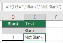
=IF(D3=»»,»Blank»,»Not Blank»)
This formula says IF(D3 is nothing, then return «Blank», otherwise «Not Blank»). Here is an example of a very common method of using «» to prevent a formula from calculating if a dependent cell is blank:
-
=IF(D3=»»,»»,YourFormula())
IF(D3 is nothing, then return nothing, otherwise calculate your formula).
Need more help?
The logical expression =»» means «is empty». In the example shown, column D contains a date if a task has been completed. In column E, a formula checks for blank cells in column D. If a cell is blank, the result is a status of «Open». If the cell contains value (a date in this case, but it could be any value) the formula returns «Closed».
The effect of showing «Closed» in light gray is accomplished with a conditional formatting rule.
Display nothing if cell is blank
To display nothing if a cell is blank, you can replace the «value if false» argument in the IF function with an empty string («») like this:
=IF(D5="","","Closed")
Alternative with ISBLANK
Excel contains a function made to test for blank cells called ISBLANK. To use the ISBLANK, you can revise the formula as follows:
=IF(ISBLANK(D5),"Open","Closed")
Содержание
- If Cell is Blank
- If Blank
- If Not Blank
- Highlight Blank Cells
- If cell is not blank
- Related functions
- Summary
- Generic formula
- Explanation
- IF function
- ISBLANK function
- LEN function
- How to Determine IF a Cell is Blank or Not Blank in Excel
- Determine if a cell is blank or not blank
- Syntax of IF function is;
- Blank Cells
- Not Blank Cells
- IF Cell is Blank (Empty) using IF + ISBLANK
- Formula to Check IF a Cell is Blank or Not (Empty)
- Alternate Formula
- How to use IF function in Excel: examples for text, numbers, dates, blanks
- IF function in Excel
- Basic IF formula in Excel
- Excel If then formula: things to know
- If value_if_true is omitted
- If value_if_false is omitted
- Using IF function in Excel — formula examples
- Excel IF function with numbers
- Excel IF function with text
- Case-sensitive IF statement for text values
- If cell contains partial text
- Excel IF statement with dates
- Excel IF statement for blanks and non-blanks
- Check if two cells are the same
- IF then formula to run another formula
- Multiple IF statements in Excel
- Nested IF statement
- Excel IF statement with multiple conditions
- If error in Excel
- Practice workbook
If Cell is Blank
Use the IF function and an empty string in Excel to check if a cell is blank. Use IF and ISBLANK to produce the exact same result.
If Blank
Remember, the IF function in Excel checks whether a condition is met, and returns one value if true and another value if false.
1. The IF function below returns Yes if the input value is equal to an empty string (two double quotes with nothing in between), else it returns No.
![]()
Note: if the input cell contains a space, it looks blank. However, if this is the case, the input value is not equal to an empty string and the IF function above will return No.
2. Use IF and ISBLANK to produce the exact same result.
![]()
Note: the ISBLANK function returns TRUE if a cell is empty and FALSE if not. If the input cell contains a space or a formula that returns an empty string, it looks blank. However, if this is the case, the input cell is not empty and the formula above will return No.
If Not Blank
In Excel, <> means not equal to.
1. The IF function below multiplies the input value by 2 if the input value is not equal to an empty string (two double quotes with nothing in between), else it returns an empty string.
![]()
2. Use IF, NOT and ISBLANK to produce the exact same result.
![]()
Highlight Blank Cells
You can use conditional formatting in Excel to highlight cells that are blank.
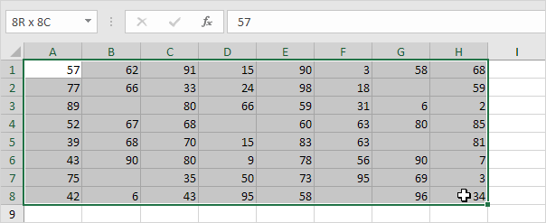
1. For example, select the range A1:H8.
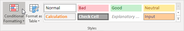
2. On the Home tab, in the Styles group, click Conditional Formatting.
3. Click Highlight Cells Rules, More Rules.
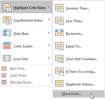
4. Select Blanks from the drop-down list, select a formatting style and click OK.
![]()
![]()
Note: visit our page about conditional formatting to learn much more about this cool Excel feature.
Источник
If cell is not blank
![]()
Summary
To test if a cell is not blank (i.e. has content), you can use a formula based on the IF function. In the example shown, the formula in cell E5 is:
As the formula is copied down it returns «Done» when a cell in column D is not blank and an empty string («») if the cell is blank.
Generic formula
Explanation
In this example, the goal is to create a formula that will return «Done» in column E when a cell in column D contains a value. In other words, if the cell in column D is «not blank», then the formula should return «Done». In the worksheet shown, column D is is used to record the date a task was completed. Therefore, if the column contains a date (i.e. is not blank), we can assume the task is complete. This problem can be solved with the IF function alone or with the IF function and the ISBLANK function. It can also be solved with the LEN function. All three approaches are explained below.
IF function
The IF function runs a logical test and returns one value for a TRUE result, and another value for a FALSE result. You can use IF to test for a blank cell like this:
In the first example, we test if A1 is empty with =»». In the second example, the <> symbol is a logical operator that means «not equal to», so the expression A1<>«» means A1 is «not empty». In the worksheet shown, we use the second idea in cell E5 like this:
If D5 is «not empty», the result is «Done». If D5 is empty, IF returns an empty string («») which displays as nothing. As the formula is copied down, it returns «Done» only when a cell in column D contains a value. To display both «Done» and «Not done», you can adjust the formula like this:
ISBLANK function
Another way to solve this problem is with the ISBLANK function. The ISBLANK function returns TRUE when a cell is empty and FALSE if not. To use ISBLANK directly, you can rewrite the formula like this:
Notice the TRUE and FALSE results have been swapped. The logic now is if cell D5 is blank. To maintain the original logic, you can nest ISBLANK inside the NOT function like this:
The NOT function simply reverses the result returned by ISBLANK.
LEN function
One problem with testing for blank cells in Excel is that ISBLANK(A1) or A1=»» will both return FALSE if A1 contains a formula that returns an empty string. In other words, if a formula returns an empty string in a cell, Excel interprets the cell as «not empty». To work around this problem, you can use the LEN function to test for characters in a cell like this:
This is a much more literal formula. We are not asking Excel if A1 is blank, we are literally counting the characters in A1. The LEN function will return a positive number only when a cell contains actual characters.
Источник
How to Determine IF a Cell is Blank or Not Blank in Excel
You may have a range of data in Excel and need to determine whether or not a cell is Blank. This article explains how to accomplish this using the IF function.
Determine if a cell is blank or not blank
Generally, the Excel IF function evaluates where a cell is Blank or Not Blank to return a specified value in TRUE or FALSE arguments. Moreover, IF function also tests blank or not blank cells to control unexpected results while making comparisons in a logical_test argument or making calculations in TRUE/FALSE arguments because Excel interprets blank cell as zero, and not as an empty or blank cell.
Syntax of IF function is;
IF(logical_test, value_if_true, value_if_false)
In IF statement to evaluate whether the cell is Blank or Not Blank, you can use either of the following approaches;
- Logical expressions Equal to Blank (=””) or Not Equal to Blank (<>””)
- ISBLANK function to check blank or null values. If a cell is blank, then it returns TRUE, else returns FALSE.
Following examples will explain the difference to evaluate Blank or Not Blank cells using IF statement.
Blank Cells
To evaluate the cells as Blank , you need to use either logical expression Equal to Blank (=””) of ISBLANK function inthe logical_test argument of the IF formula. In both methods logical_test argument returns TRUE if a cell is Blank, otherwise, it returns FALSE if the cell is Not Blank
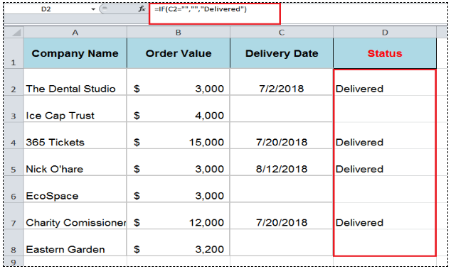
For example, you need to evaluate that if a cell is Blank, the blank value, otherwise return a value “Delivered” . In both approaches, following would be the IF formula;
In both of the approaches, logical_test argument returns TRUE if a cell is Blank, and the value_if_true argument returns the blank value. Otherwise, the value_if_false argument returns value “Delivered”.

Not Blank Cells
To evaluate the cells are Not Blank you need to use either the logical expression Not Equal to Blank (<>””) of ISBLANK function in logical_test argument of IF formula. In case of logical expression Not Equal to Blank (<>””) logical_test argument returns TRUE if the cell is Not Blank, otherwise, it returns FALSE. In case of the ISBLANK function, the logical_test argument returns FALSE if a cell is Not Bank. Otherwise it returns TRUE if a cell is blank.
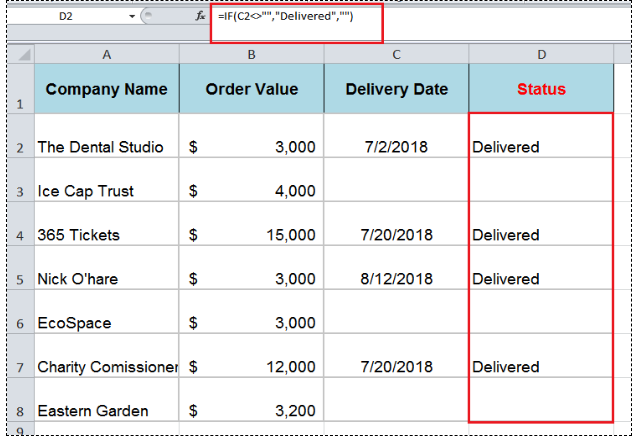
For example, you need to evaluate that if a cell is Not Blank, then return a value “ Delivered ” , otherwise return a blank value. In both approaches, following would be the IF formula;
In this approach, the logical expression Not Equal to Blank (<> “” ) returns TRUE in the logical_test argument if a cell is Not Blank, and the value_if_true argument returns a value “Delivered” , otherwise value_if_false argument a blank value.
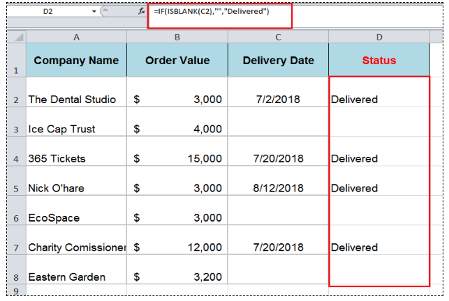
This approach is opposite to first one above. In IF formula, ISBLANK function returns FALSE in the logical_test argument if a cell is Not Blank, so value_if_true argument returns blank value and a value_if_false argument returns a value “Delivered” .
Still need some help with Excel formatting or have other questions about Excel? Connect with a live Excel expert here for some 1 on 1 help. Your first session is always free.
Are you still looking for help with the IF function? View our comprehensive round-up of IF function tutorials here.
Источник
IF Cell is Blank (Empty) using IF + ISBLANK
In Excel, if you want to check if a cell is blank or not, you can use a combination formula of IF and ISBLANK. These two formulas work in a way where ISBLANK checks for the cell value and then IF returns a meaningful full message (specified by you) in return.
In the following example, you have a list of numbers where you have a few cells blank.
![]()
Formula to Check IF a Cell is Blank or Not (Empty)
- First, in cell B1, enter IF in the cell.
- Now, in the first argument, enter the ISBLANK and refer to cell A1 and enter the closing parentheses.
- Next, in the second argument, use the “Blank” value.
- After that, in the third argument, use “Non-Blank”.
- In the end, close the function, hit enter, and drag the formula up to the last value that you have in the list.
![]()
As you can see, we have the value “Blank” for the cell where the cell is empty in column A.
Now let’s understand this formula. In the first part where we have the ISBLANK which checks if the cells are blank or not.
![]()
And, after that, if the value returned by the ISBLANK is TRUE, IF will return “Blank”, and if the value returned by the ISBLANK is FALSE IF will return “Non_Blank”.
![]()
Alternate Formula
You can also use an alternate formula where you just need to use the IF function. Now in the function, you just need to specify the cell where you want to test the condition and then use an equal operator with the blank value to create a condition to test.
And you just need to specify two values that you want to get the condition TRUE or FALSE.
Источник
How to use IF function in Excel: examples for text, numbers, dates, blanks
 by Svetlana Cheusheva, updated on September 20, 2022
In this article, you will learn how to build an Excel IF statement for different types of values as well as how to create multiple IF statements.
IF is one of the most popular and useful functions in Excel. Generally, you use an IF statement to test a condition and to return one value if the condition is met, and another value if the condition is not met.
In this tutorial, we are going to learn the syntax and common usages of the Excel IF function, and then take a closer look at formula examples that will hopefully prove helpful to both beginners and experienced users.
IF function in Excel
IF is one of logical functions that evaluates a certain condition and returns one value if the condition is TRUE, and another value if the condition is FALSE.
The syntax of the IF function is as follows:
As you see, IF takes a total of 3 arguments, but only the first one is obligatory, the other two are optional.
Logical_test (required) — the condition to test. Can be evaluated as either TRUE or FALSE.
Value_if_true (optional) — the value to return when the logical test evaluates to TRUE, i.e. the condition is met. If omitted, the value_if_false argument must be defined.
Value_if_false (optional) — the value to return when the logical test evaluates to FALSE, i.e. the condition is not met. If omitted, the value_if_true argument must be set.
Basic IF formula in Excel
To create a simple If then statement in Excel, this is what you need to do:
- For logical_test, write an expression that returns either TRUE or FALSE. For this, you’d normally use one of the logical operators.
- For value_if_true, specify what to return when the logical test evaluates to TRUE.
- For value_if_false, specify what to return when the logical test evaluates to FALSE. Though this argument is optional, we recommend always configuring it to avoid unexpected results. For the detailed explanation, please see Excel IF: things to know.
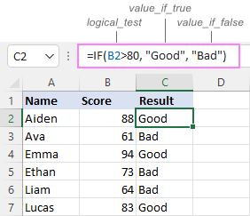
As an example, let’s write a very simple IF formula that checks a value in cell A2 and returns «Good» if the value is greater than 80, «Bad» otherwise:
=IF(B2>80, «Good», «Bad»)
This formula goes to C2, and then is copied down through C7:
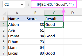
In case you wish to return a value only when the condition is met (or not met), otherwise — nothing, then use an empty string («») for the «undefined» argument. For example:
This formula will return «Good» if the value in A2 is greater than 80, a blank cell otherwise:
Excel If then formula: things to know
Though the last two parameters of the IF function are optional, your formula may produce unexpected results if you don’t know the underlying logic.
If value_if_true is omitted
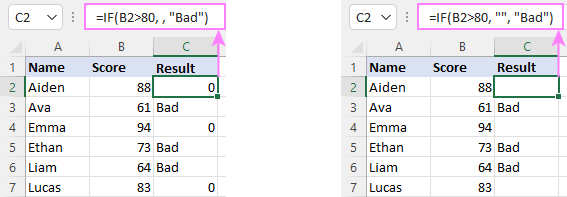
If the 2 nd argument of your Excel IF formula is omitted (i.e. there are two consecutive commas after the logical test), you’ll get zero (0) when the condition is met, which makes no sense in most cases. Here is an example of such a formula:
To return a blank cell instead, supply an empty string («») for the second parameter, like this:
The screenshot below demonstrates the difference:
If value_if_false is omitted
Omitting the 3 rd parameter of IF will produce the following results when the logical test evaluates to FALSE.
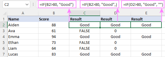
If there is just a closing bracket after value_if_true, the IF function will return the logical value FALSE. Quite unexpected, isn’t it? Here is an example of such a formula:
Typing a comma after the value_if_true argument will force Excel to return 0, which doesn’t make much sense either:
The most reasonable approach is using a zero-length string («») to get a blank cell when the condition is not met:
Tip. To return a logical value when the specified condition is met or not met, supply TRUE for value_if_true and FALSE for value_if_false. For the results to be Boolean values that other Excel functions can recognize, don’t enclose TRUE and FALSE in double quotes as this will turn them into normal text values.
Using IF function in Excel — formula examples
Now that you are familiar with the IF function’s syntax, let’s look at some formula examples and learn how to use If then statements in real-life scenarios.
Excel IF function with numbers
To build an IF statement for numbers, use logical operators such as:
- Equal to (=)
- Not equal to (<>)
- Greater than (>)
- Greater than or equal to (>=)
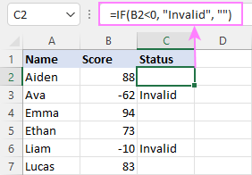
- Less than ( =IF(B2
For negative numbers (which are less than 0), the formula returns «Invalid»; for zeros and positive numbers — a blank cell.
Excel IF function with text
Commonly, you write an IF statement for text values using either «equal to» or «not equal to» operator.
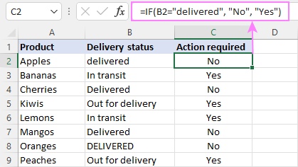
For example, the following formula checks the Delivery Status in B2 to determine whether an action is required or not:
=IF(B2=»delivered», «No», «Yes»)
Translated into plain English, the formula says: return «No» if B2 is equal to «delivered», «Yes» otherwise.
Another way to achieve the same result is to use the «not equal to» operator and swap the value_if_true and value_if_false values:
=IF(C2<>«delivered», «Yes», «No»)
- When using text values for IF’s parameters, remember to always enclose them in double quotes.
- Like most other Excel functions, IF is case-insensitive by default. In the above example, it does not differentiate between «delivered», «Delivered», and «DELIVERED».
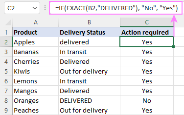
Case-sensitive IF statement for text values
To treat uppercase and lowercase letters as different characters, use IF in combination with the case-sensitive EXACT function.
For example, to return «No» only when B2 contains «DELIVERED» (the uppercase), you’d use this formula:
=IF(EXACT(B2,»DELIVERED»), «No», «Yes»)
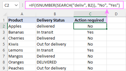
If cell contains partial text
In situation when you want to base the condition on partial match rather than exact match, an immediate solution that comes to mind is using wildcards in the logical test. However, this simple and obvious approach won’t work. Many functions accept wildcards, but regrettably IF is not one of them.
A working solution is to use IF in combination with ISNUMBER and SEARCH (case-insensitive) or FIND (case-sensitive).
For example, in case «No» action is required both for «Delivered» and «Out for delivery» items, the following formula will work a treat:
=IF(ISNUMBER(SEARCH(«deliv», B2)), «No», «Yes»)
For more information, please see:
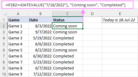
Excel IF statement with dates
At first sight, it may seem that IF formulas for dates are akin to IF statements for numeric and text values. Regrettably, it is not so. Unlike many other functions, IF does recognize dates in logical tests and interprets them as mere text strings. In other words, you cannot supply a date in the form of «1/1/2020» or «>1/1/2020». To make the IF function recognize a date, you need to wrap it in the DATEVALUE function.
For example, here’s how you can check if a given date is greater than another date:
=IF(B2>DATEVALUE(«7/18/2022»), «Coming soon», «Completed»)
This formula evaluates the dates in column B and returns «Coming soon» if a game is scheduled for 18-Jul-2022 or later, «Completed» for a prior date.
Of course, there is nothing that would prevent you from entering the target date in a predefined cell (say E2) and referring to that cell. Just remember to lock the cell address with the $ sign to make it an absolute reference. For instance:
=IF(B2>$E$2, «Coming soon», «Completed»)
To compare a date with the current date, use the TODAY() function. For example:
=IF(B2>TODAY(), «Coming soon», «Completed»)
Excel IF statement for blanks and non-blanks
If you are looking to somehow mark your data based on a certain cell(s) being empty or not empty, you can either:
- Use the IF function together with ISBLANK, or
- Use the logical expressions =»» (equal to blank) or <>«» (not equal to blank).
The table below explains the difference between these two approaches with formula examples.
Evaluates to TRUE if a cell is visually empty, even if it contains a zero-length string.
Otherwise, evaluates to FALSE.
Evaluates to TRUE is a cell contains absolutely nothing — no formula, no spaces, no empty strings.
Otherwise, evaluates to FALSE.
| Logical test | Description | Formula Example | |
| Blank cells | =»» | =IF(A1=»», 0, 1)
Returns 0 if A1 is visually blank. Otherwise returns 1. If A1 contains an empty string («»), the formula returns 0. |
|
| ISBLANK() | =IF( ISBLANK(A1) , 0, 1)
Returns 0 if A1 is absolutely empty, 1 otherwise. If A1 contains an empty string («»), the formula returns 1. |
||
| Non-blank cells | <>«» | Evaluates to TRUE if a cell contains some data. Otherwise, evaluates to FALSE.
Cells with zero-length strings are considered blank. |
=IF( A1<>«», 1, 0)
Returns 1 if A1 is non-blank; 0 otherwise. If A1 contains an empty string, the formula returns 0. |
| ISBLANK() =FALSE | Evaluates to TRUE if a cell is not empty. Otherwise, evaluates to FALSE.
Cells with zero-length strings are considered non-blank. |
=IF( ISBLANK(A1) =FALSE, 0, 1)
Works the same as the above formula, but returns 1 if A1 contains an empty string. |
And now, let’s see blank and non-blank IF statements in action. Suppose you have a date in column B only if a game has already been played. To label the completed games, use one of these formulas:
In case the tested cells have no zero-length strings, all the formulas will return exactly the same results:
![]()
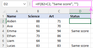
Check if two cells are the same
To create a formula that checks if two cells match, compare the cells by using the equals sign (=) in the logical test of IF. For example:
=IF(B2=C2, «Same score», «»)
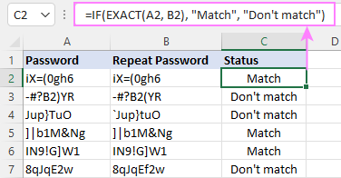
To check if the two cells contain same text including the letter case, make your IF formula case-sensitive with the help of the EXACT function.
For instance, to compare the passwords in A2 and B2, and returns «Match» if the two strings are exactly the same, «Do not match» otherwise, the formula is:
=IF(EXACT(A2, B2), «Match», «Don’t match»)
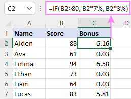
IF then formula to run another formula
In all of the previous examples, an Excel IF statement returned values. But it can also perform a certain calculation or execute another formula when a specific condition is met or not met. For this, embed another function or arithmetic expression in the value_if_true and/or value_if_false arguments.
For example, if B2 is greater than 80, we’ll have it multiplied by 7%, otherwise by 3%:
Multiple IF statements in Excel
In essence, there are two ways to write multiple IF statements in Excel:
- Nesting several IF functions one into another
- Using the AND or OR function in the logical test
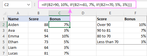
Nested IF statement
Nested IF functions let you place multiple IF statements in the same cell, i.e. test multiple conditions within one formula and return different values depending on the results of those tests.
Assume your goal is to assign different bonuses based on the score:
- Over 90 — 10%
- 90 to 81 — 7%
- 80 to 70 — 5%
- Less than 70 — 3%
To accomplish the task, you write 3 separate IF functions and nest them one into another like this:
=IF(B2>90, 10%, IF(B2>=81, 7%, IF(B2>=70, 5%, 3%)))
For more formula examples, please see:
Excel IF statement with multiple conditions
To evaluate several conditions with the AND or OR logic, embed the corresponding function in the logical test:
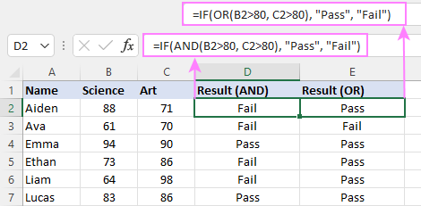
For example, to return «Pass» if both scores in B2 and C2 are higher than 80, the formula is:
=IF(AND(B2>80, C2>80), «Pass», «Fail»)
To get «Pass» if either score is higher than 80, the formula is:
=IF(OR(B2>80, C2>80), «Pass», «Fail»)
For full details, please visit:
If error in Excel
Starting from Excel 2007, we have a special function, named IFERROR, to check formulas for errors. In Excel 2013 and higher, there is also the IFNA function to handle #N/A errors.
And still, there may be some circumstances when using the IF function together with ISERROR or ISNA is a better solution. Basically, IF ISERROR is the formula to use when you want to return something if error and something else if no error. The IFERROR function is unable to do that as it always returns the result of the main formula if it isn’t an error.
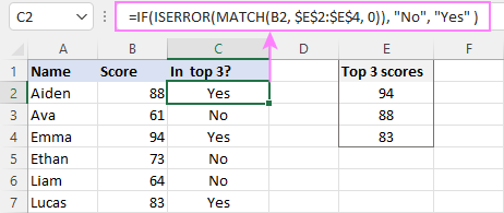
For example, to compare each score in column B against the top 3 scores in E2:E4, and return «Yes» if a match is found, «No» otherwise, you enter this formula in C2, and then copy it down through C7:
=IF(ISERROR(MATCH(B2, $E$2:$E$4, 0)), «No», «Yes» )
For more information, please see IF ISERROR formula in Excel.
Hopefully, our examples have helped you get a grasp of the Excel IF basics. I thank you for reading and hope to see you on our blog next week!
Practice workbook
Table of contents
I want to highlight column A one color depending on specific name in column G of the same line.
Hello!
The answer to your question can be found in this article: Excel conditional formatting formulas based on another cell.
Hi, I am trying to write an if-formula where, if the value is true, the outcome should but 0, but if the outcome is false, a formula should calculate a value. So far this is what I have got: «=IF(F4=»Yes»,0,(G4+J4)-(E4+H4+I4))». However, this does not work. Is this idea possible or should I implement this in a different way?
I got it! The answer was «=IF(F4=»Yes»;0;(G4+J4)-(E4+H4+I4))»
Hello, good day!
I need a formula for my sheet that automatically updates my cell as «Updated Recently» if the date I entered is within this week, if not it should be automatically update with just a blank.
For example:
[Cell1] Last Sale: March 10 (within a week) = [Cell2] Status: Updated Recently
[Cell1] Last Sale: Feb 27 (Last week/last month) = [Cell2] Status:
Hello!
Use the WEEKNUM function to get the week number for each date and compare them.
This should solve your task.
What shall I write in logic test,value true and value false while doing my ecxel program
**Correction to my previous question: need help with this formula- If the date in cell W2 > date in cell Q2, then return the number that is in cell AB2, if not then return number in cell T2
Try this formula —
IF(W2 > Q2,AB2,T2)
need help with this formula- If the date in cell W2 > date in cell Q2, then return the number that is in column T2
Hi!
All the necessary information is in the article above. Since the dates in Excel are numbers, you can compare them as numbers.
I want help writing a formula where on an expenditure sheet there are two ‘company names’ which amounts spent ge assigned to. The formula I require is to automatically take the amounts from the other sheet and list the amount assigned to either company on diiferent cells under the heading of the company name.
Hello!
You can get a list of amounts for each company using the FILTER function. You can find the examples and detailed instructions here: Excel FILTER function — dynamic filtering with formulas.
Hi. I need a formula to populate the name of the counselor assigned to a student based on a students last name. I have a list of student’s last names on column G and I have the the counselors names on a different sheet within the same workbook. Please help. I got it to work if I place the counselors names on the same sheet where the student information is located but if I delete a student, it will mess with the formula.
Hello!
If I understand your task correctly, the following tutorial should help: How to VLOOKUP between two sheets. If you receive a #N/A! error, this article will be helpful: IFERROR & VLOOKUP — trap #N/A and other errors. I hope I answered your question. If something is still unclear, please feel free to ask.
Hi, Im trying to find a formula to search from column D2 to D10 for an exact name if there is to print yes if not to print no.
First name Last name
1 John Smith
2 Mike Hunt
3 Sam Isaco
So basically what I want to do is if the certain name and last name are found in these columns to print yes
Is this possible?
Hello!
If I understand your task correctly, you can define a partial match of a word and a text string with the combination ISNUMBER + SEARCH functions.
I hope it’ll be helpful. If this is not what you wanted, please describe the problem in more detail.
Hi, Can you please help me, in Excel if column A2 value= Column B value, then only compare column C value with column D value and provide result in column E.
Example:
1234 END 1234 CERIAL END
1234 FORNT 1234 BACK FRONT
1234 ARIAL 1234 GAME9 N/A
1234 GAME 1234 GAME2 GAME2
1234 GAME 6 1234 GAME8 N/A
1234 GAME9 1234 GAME7 GAME9
1234 GAME2 1234 FRONT N/A
1234 GAME3 1234 CHANG N/A
1234 GAME1 1234 END N/A
I’m not sure if anyone can help with what I think should be a relative simple formula that I’m stuck on. I need to create and IF or an AND formula that will look at two arguments that both need to be be True, one argument is checking that a Date is =>2023,1,1 and another cell contains an exact text «Vacancy».
I have managed to get the Date check to work, however I have no idea how to add the AND argument to check the text in the other cell, I currently have the following formula:
The person should only be entitled to the payment if the Date is >=2023,1,1 and that the Role (text) in cell B2 is «Vacancy».
Thank you for your help.
Hi!
Add another condition to the formula using the logical AND operator. See here for detailed instructions: IF AND formula in Excel.
Brilliant! Thank you so much for your help, this has worked perfectly. I could not work out where the AND should go. Thank you.
How can i categorize the cell content based on the starting letter. (Example:- Different grade of fruits has code like a123, b123 etc., i want to categorize the fruits as «A grade» for the code that starts with «a».
Hi!
The information you provided is not enough to recommend you a formula. To extract the first character from the code, use the LEFT function.
LEFT(A1,1)
Thank for your prompt response Mr. Alexander
i have list of materials in row A which has two types of material codes one type starts with alphabet like «S123, S234 and so on» which is semi finished and another code was only numeric it was finished goods. In row D i need the codes which starts with alphabetic should name as «Semifinished» and numeric code as «Finished goods». i believe that i gave you the clarity to derive the formula.
Hello!
This formula returns TRUE if the first character is a letter.
I hope this will help, otherwise don’t hesitate to ask.
Yes, it’s working but it will be convenient if the formula returns to any name instead of TRUE or FALSE.
Hi!
If you want to get a list of all alphabetic codes, use the FILTER function. For example,
I have 3 options in source column instead of two so how should I do
For example
If IND2522 — it should reflect in colour as India
If BNG2522 — it should be reflect as Bangladesh
If PAK2522 — it should be reflect as Pakistan
Hi! Please clarify your specific problem or provide additional details to highlight exactly what you need. As it’s currently written, it’s hard to tell exactly what you’re asking.
Logical Text in A1 Cell ,TRUE Value in A2 and FALSE Value in A3
i write IF Function in A4 = IF(A1,A2,A3)
but it doesn’t work properly. it will prompt Error Massage (#Value!)
so can i put LOGICAL TEXT in cell.
Hi!
Read the article above carefully. What is written in A1? I think it’s just plain text.
Hello. Please help provide the formula for a cell L23 to either show «N» if less than a certain date such as 02/15/2023 and «N» if passed that date in A23, thank you!
Hi!
Pay attention to the following paragraph of the article above: Excel IF statement with dates.
It covers your case completely.
Donno if this Forum works now:
I am trying to figure out a formula for the following:
I have 3 Columns : viz : A1,D1, L1 with text contents. And output expected in M1
So if All of the 3 cells A,D,L are Blank, Then out put should be «Spare»,
If any of the 3 cells mentions : «In Stock», Output should be «In Stock»,
If any of the 3 cells mentions : «Faulty», Output should be «Faulty»,
Else if any columns has any text it should show » Mapped»
Hi!
Combine cell values and search for the desired text using the SEARCH function. Use a nested IF function to display values based on conditions.
Try this formula:
=IF(ISNUMBER(SEARCH(«In Stock»,A1&D1&L1)),»In Stock», IF(ISNUMBER(SEARCH(«Faulty»,A1&D1&L1)),»Faulty», IF(A1&D1&L1=»»,»Spare»,»Mapped»)))
i need to calculate the hours of the roster of the month of each staff (M=6.5, E=6.5 , N=8, O=0) please help
Hi!
I am not sure I fully understand what you mean.
Hi!
I am trying to get my IF statement to take a current number, and if it is over 40, bring it down to 40. If it is under 40 I want to leave it at 40.
I have attempted the formula =IF(E10>40, 40, E10) I just don’t know what to put in the false statement, to keep it at the current value it was at if under 40.
Thanks for the help!
Hi!
Your formula keeps the current value if it’s less than 40.
=IF(B1=5 and C1=3, «Good combination», how i can use this formula
Hi!
You can find the answer to your question in this article: IF AND formula in Excel.
I’m trying to create a formula to help build a table for a student outcome report.
A B C D
1 Comm 1010 Comm 2010 Comm 3000
2 Communication 2 4
3 Critical/Creative Thinking 5
4 Community Awareness 3 4
If any text in Column A=Communication and any text in Row 1= Comm 1010, then show the number for that combination. In this example, 2 would be displayed.
If any text in Column A=Critical* and any text in Row 1=Comm 2010*, then show the number for that combination. In this example, 5 would be displayed. I need to be able to use a wildcard for both text options.
If there is no number in the cell, then leave it blank.
The numbers will be sent to a different sheet. Right now, I have to sort both sheets so everything lines up. I am hoping there is a formula that will pull over the numbers and I don’t have to sort anything.
Hello!
You can do an approximate search using the SEARCH and ISNUMBER functions. Also use this instruction: Excel INDEX MATCH MATCH and other formulas for two-way lookup.
For example, instead of the formula
=INDEX(B2:E4, MATCH(H1, A2:A4, 0), MATCH(H2, B1:E1, 0))
use the formula
=INDEX(B2:E4, MATCH(TRUE,ISNUMBER(SEARCH(H1,A2:A4)),0), MATCH(TRUE,ISNUMBER(SEARCH(H2,B1:E1)),0))
I hope my advice will help you solve your task.
Can you help? What is the correct IF formula for — Should Grunar continue to make the part or buy it from the supplier? #2 question below.
Complete the schedule to support the decision of whether to make or buy the part.
Relevant Costs to Make Relevant Cost to Buy
Direct materials $2.80
Direct labor 1.70
Variable manufacturing overhead 0.50
Fixed manufacturing overhead 0.40
Total cost $5.40 $6.25
#2. Should Grunar continue to make the part or buy it from the supplier?
Grunar should
** Function: IF; Cell reference.
Input the IF function with cell references to this work with output of «make the part.» and «buy the part.» for the decision.
Hi!
Have you tried the ways described in this blog post? Please read the above article carefully.
Hello, good day,
I want to extract in sheet 1 from sheet 2 the value(text) and is if there is not text to writre no text, or if is blank to write no text, sample.
Sheet 2 FM «NAME», copy in sheet 1 that name, and if there is not name to write «No Name», i try many ways and always i have error, i try with
=if(Sheet2!C15=»»,»»,»No mane») but don’t copy the name if is there. as well =TEXT(Claudio!C15,IF(ISBLANK(Claudio!C15),»NO FM»))
please can you help me,
Hi!
All the necessary information is in the article above.
If I understand your task correctly, try the following formula:
0 points if the employee age is less than 27.
5 points if the employee age is between 27 and 30.
10 points if the employee age is between 30 and 33.
15 points if the employee age is between 33 and 35.
SDP:
0 points if the employee is not an SP.
15 points if the employee is an Sp
GPA:
5 points if the employee GPA is between 2 and 2.3.
10 points if the employee GPA is between 2.3 and 2.5.
15 points if the employee GPA is between 2.5 and 2.7.
20 points if the employee GPA is between 2.7 and 2.9.
25 points if the employee GPA is greater than 2.9.
Hi!
If I understand your task correctly, the following tutorial should help: Excel Nested IF statements — examples, best practices and alternatives.
hi i want to create a formula =if(colum A:A=name of a product = colum B:B) is it posible?
Hi!
Please clarify your problem and provide additional details to highlight exactly what you need. As it’s currently written, it’s hard to tell exactly what you’re asking.
I have an xlookup (in ‘Bill 1-9-23’!E2) is used to find a three letter code (AIHP or UCH) in col E of ‘Client Roster’, that works :
=XLOOKUP(‘Bill 1-9-23′!A2,’Client Roster’!A:A,’Client Roster’!E:E,»»)
Then in ‘Bill 1-9-23’!G2 I want to use an IF to determine if I found AIHP or UCH and make different results, so:
=IF(E2=»AIHP»,500,350)
It always returns 350 (FAILED), even when E2 is displaying AIHP.
If I enter a number in Client Roster’!E2 and logically test against that, then it works.
Thank you for yourhelp, in advance.
LH
Hi!
Check the values in column A for extra spaces and nonprinting characters.
Maybe this article will be helpful: How to remove spaces in Excel — leading, trailing, non-breaking
I’m trying to work on a formula; say
I type in the value 5857 in D12
Then, if the value i typed has it’s first three values matching the first three values of any cell in the range A2:A35 counting from the left, pick the corresponding value on the right
So if the one I entered has its first three values counting from the left matching that of A14. Both values are matching 587, it will pick the corresponding value on B14 then add it to the cell C8
i did something like this
=IF(AND(LEFT(A18:A213,3)=LEFT(A2,3),RIGHT(A2,1)=»0″),B18:B213+C8, IF(AND(LEFT(A18:A213,3)=LEFT(A2,3),RIGHT(A2,1)=»1″),B18:B213+C8))
and I’m getting
#VALUE
Hi!
Your formula does not match the question. Therefore, your problem is difficult to understand. Note, however, that LEFT(A18:A213,3)=LEFT(A2,3) returns not a single value, but an array of 195 values.
hi. I have 1 problem
cell 1 cell 2
we have text in 1 cell, bellow that cell we want some respective numbers with that text. ex1. A 1
B 2
C 3
AND WE CREATED FOR CELL 1 DROPDOWN LIST SO PLEASE HELP ME. AS SOON AS POSSIBLE
THANKS
Hi Alex,
I am trying to build an IF function that will select beneficiaries based on set of criteria. Below is the Formula I have used =IF(T35,IF(BD3=»Yes»,IF(BE3 Reply
Hi!
Read this guide carefully: Nested IF in Excel – formula with multiple conditions.
T35 is not a condition. Don’t forget to separate the arguments of the IF function with commas.
Hi Alexander,
I am attempting to streamline repetitive data entry by using Sheet 1 as a ‘controlled data’ sheet, where data can be identified and automatically transferred across to new worksheets/cells when data is being entered. I’d like the active cells to recognise various text codes such as EDT01, EDT02, EDT03,etc, and transfer selected information from various cells across to the same cell location in the new work sheet.
In essence, when entering data for EDT01 into the new worksheet, columns C2, D2 and E2 will have the same specific size dimensions, therefore rather than continually typing in these dimensions for multiple entries, it would be beneficial to have the code EDT01 identified when typed and the size dimensions automatically filled into these specific columns.
I’m struggling to explain this in any great detail but hope you get the gist of my problem.
Thanks you in advance.
Hi!
I think your problem can be solved either with an IF formula or a VBA macro.
I’m trying to work on a formula to say if B22 is equal to 12 multiply the number in D22 by 2, and if B23 is equal 12 then multiply the number in D23 by 2. So on until B30. But if the numbers in B22 to B30 don’t contain 12 leave the cell blank. I have the following formula which returns the result FALSE instead of blank.
Can you help on this?
Hello!
If I understand your task correctly, use SUMPRODUCT function:
I need formula for condition
if condition in J15 column is «returned» Than F15=0
otherwise, it should remain same please make formula for this situation
Hi,
Need a help I have list of activity on cell B (72 activity) and in cell E (Planned date) and F (Actual date) how I’ll get the data from cell B if if my actual date is blank and formula will get the data from activity what we have before the blank cell.
Hi!
Please clarify your specific problem or provide additional information to understand what you need.
I have created a simple if then statement to check for text within a range.
However, the statement is always returned «false» even when no data is present in the range of cells.
If I remove the range & check only 1 cell at a time, the function works as expected.
=IF((ISBLANK(H3:H500)), «THIS COMPANY MUST SHOW A PAID IN FULL INVOICE BEFORE SENDING STAMPED PLANS OF ANY SORT», «SOMETHING NEEDS TO BE SENT»)
I figured it out using «COUNTA»
=IF(COUNTA(H3:H994)= 0, «THIS COMPANY MUST SHOW A PAID IN FULL INVOICE BEFORE SENDING STAMPED PLANS OF ANY SORT», «SOMETHING NEEDS TO BE SENT»)
Hi!
If the cell contains a value, the formula returns FALSE
If there is no data — TRUE
Try to enter the formula as an array formula.
Goodmorning all, i am trying to create an if formula that can generate a letter code for a given amperage. =IF(I9=380,»P»,IF(I9=300,»O»,IF(I9=290,»N»,IF(I9=230,»M»,IF(I9=200,»L»,IF(I9=180,»K»,IF(I9=150,»J»,IF(I9=130,»I»,IF(I9=120,»ZZ»,IF(I9=100,»H»,IF(I9=90,»G»,IF(I9=80,»F»,IF(I9=70,»E»,IF(I9=60,»D»,IF(I9=40,»C»,IF(I9=30,»B»,IF(I9=20,»A»,IF(I9=10,»A»,»NOPE»)))))))))))))))))) this is working great but now i want to use that answer from that if statement to reference another cell with A corresponding letter for the wire size answer. is there a formula that can refence a that letter and match it to the given answers on another column?
Hi!
To create a link to another cell from text, use the INDIRECT function.
I hope it’ll be helpful. If this is not what you wanted, please describe the problem in more detail.
Thank you for the suggestion!! i was able to get the result that i desired using this formula!
the idea was to use if statements to generate a letter code based on amperage and a sub code based on phases, with the above formula i was able to convert the codes into indirectly referencing the wire size text in another cell. Works like a charm.
Hi
I want to have information on a spreadsheet that displays everything but when you change an option that i have created lists for it displays in the corresponding worksheet also.
So I want a list of all computers and their details, on separate tabs below will be named faulty, operational, sent to maintenance etc.
I’ve created a list on the All sheet with a drop down box but when I select an option I want it to also display the entire row of data to the sheet with the same name.
I just don’t know how to formulate it sorry could you please advise
If G# (between R3 — 300) = set value (Operational, Faulty, Sent for repair) copy row from column B:AU «tab All» to «Tab ###»
Hope this makes sense
Thanks in advance
Rob
Hi!
I’m not sure I got you right since the description you provided is not entirely clear. Maybe this article will be helpful: Excel FILTER function — dynamic filtering with formulas.
Thank you for the quick reply, sorry this was an extremely poor way to explain my issue
I’ll try and explain it better,
I’m trying to use a spreadsheet to keep track of data on near 300 pieces of equipment with each piece having 50+ columns of information on. I’ve used data validation to create lists on certain columns to have fixed data inputs available. on sheet 1 I have all the information but what I’d like is to be able to create extra sheets with the same names as that on the Lists and as someone changes the value in the dropdown list then it copies automatically to sheet with the corresponding name.
i want it to be the entire row of information though.
the manual way to do this is to filter the search to the set value copy and paste across, I just wonder if there was an automatic way to do it with a
protected worksheet so when different people update it I doesn’t mess with the formula and I don’t have to come and do an audit regularly to make sure it has been transferred over properly
hope this makes more sense
Hello!
On each additional sheet, you can create a table for specific equipment using the FILTER function, or use a pivot table.
Hi, I am trying to create an IF formula.
I am trying to find a way to build an IF formula like that: If you see a date, tell me what is the date, and if you don’t, tell me the previous date.
So I am trying to create this formula in the B row. In the C row there are dates and cities.
Short exemple: C2=Apr/19, C3=NY, C4=Miami, C5=Apr/20
I want B2,B3,B4 to tell me Apr/19 and B5 to tell me Apr 20.
Hi!
You can determine the date in a cell using the ISNUMBER function. To find the last date in a range, use XLOOKUP function.
I believe the following formula will help you solve your task:
I have an inquiry and would appreciate your expertise, if time permits.
I’m trying to formulate a rule that if a value resides in a defined row, for example A1, B1, C1, D1, then mark/color that specific value throughout the rest of the Excel sheet.
For example:
A1, B1, C1, D1 — mark any value in this row Blue
A2, B2, C2, D2 — mark any value in this row Red
B3, C3, D3 — mark any value in this row Green
However, it also needs to be Top Down Authoritative, where if a value exists in a preceding row, for example Row 1 (A1, B1, C1, D1), that value is ignored for being marked/colored in the proceeding rows.
Is this possible with an IF function?
Hello!
Unfortunately, I don’t really understand what you want to do. However, you may find it useful to have a custom function that gets the cell color. See the code and examples at this link.
Hello, I would like your advice.
How would I write a formula that displays a specific value in one cell, if the value in another cell matches.
I am trying to make the raw data received from a survey more palatable. So I have a survey question that (for examples asks you to choose your favorite color from list of 13 colors. I want to use a formula that I can place in cell C1 that displays the value in B4 if the value in A1 is 4, but I want that for all the values.
The logic is as follows: IF A=1 «display B1» AND IF A=2 «display B2» AND IF A=3 «display B3» (. and so on and so forth)
Thank you in advance!
Hello!
You can use the CHOOSE function to select one of the many options.
I hope it’ll be helpful.
Hello, Thank you this is exactly what i need!
Is there a way to use the CHOOSE function (or VLOOKUP or INDEX or MATCH) to display a value if the index cell has multiple values separated by commas?
For example: Cell A1 has the values 1, 4, 5 in that cell. but I would still like for the logic to operate as follows: IF A=1 «display B1» AND IF A=2 «display B2» AND IF A=3 «display B3» (. and so on and so forth)
Hello!
If I understand correctly, to extract the first number from a text string, use the LEFT function.
=CHOOSE(—LEFT(A1, SEARCH(«,», A1)-1),B1,B2,B3,B4,B5,B6,B7,B8,B9,B10)
Hi!
I use the IF function to normalize some data and give a number between 0 and 5. I have multiple IF functions of different data groups. I would like to make an average of the results from the IF functions, but I get an #DIV/0! error. I use the AVERAGE function. I believe the problem is that the result of the IF function is not in a number format, but I cannot figure out how to change it. Can you help?
Br Anne-Sofie
Hi!
Various ways to convert text to number can see in this article. I hope it’ll be helpful. If something is still unclear, please feel free to ask.
If A1=7 and B1=35
then I want to this answer C1=0 and D1=5
please help me
Hi!
All the necessary information is in the article above. Please note that each cell must have its own formula.
Hi,
Is there an option to publish value of the cell instead of the cell name in If condition.
The formula is
=IF(F9>0, «F9», IF(E9>0, «E9″, IF(D9>0,»D9», IF(C9>0, «C9»))))
Here I want to return the values of cells c9/d9/e9/f9 respectively. Thanks!
Hi!
Remove the quotes from the formula.
hi alex!, how are you, hope your doing fine, i have problem on my simple IF condition, i want to display the actual time upon updating a transaction but every rows that i updated it will give me the same time result. I’ve used the below condition and i hope you can share to me the correct formula.
=If(A1″»,now(),»») (not equal to blank)
Hi!
If I understand correctly, you want to get an unchangeable timestamp.
To prevent your date from automatically changing, you can use several methods:
1. Use Shortcuts to insert the current date and time
2. Use the recommendations from this article in our blog.
3. Replace the date and time returned by the TODAY function with their values. Copy the date (CTRL + C), then paste only the values using Paste Special or Shortcut CTRL + ALT + V.
Hi. How do I format my IF formula to return a numerical value instead of text? I need to sum all the values that are generated from my IF formula, but because the formula returns the values as «text» and not a «number» I cannot use my sum formula. Please advise. Thank you.
Hello!
I read some articles but still cant find my answer. I want to kind of like create a data base for C where we have «example1,example2,example3 etc.»
when example1 is written in C add number 15 in L
when example3 is written n C add number 30 in L
Is there a way I can do that? Thank you for your time!
Hi!
Use Excel Nested IF statements. Follow the link for detailed explanations and examples.
I have data in column F and data in column U, with dates in column S. I’m trying to have the date in column S copy to another cell on another workbook, if exact matches are found for columns F and U on the same row.
Hello!
You use two criteria to search for a value. You can find examples and explanations in this article: Excel INDEX MATCH with multiple criteria — formula examples.
I hope I answered your question. If something is still unclear, please feel free to ask.
I am trying to have an excel report something as below for «Overall Status» for each username (e.,g User1). I would like to create condition to track the overall status in which even if one of the Status is «Not Completed», mark it as «Not Completed» for each username grouped (e.,g User1). Appreciate if you could provide some inputs on this.
UserName App Status Overall Status
User1 App1 Completed Not Completed
User1 App2 Not Completed
User1 App3 Completed
User1 App4 Not Completed
User1 App5 Completed
User2 App1 Completed Not Completed
User2 App2 Completed
User2 App3 Not Completed
User2 App4 Completed
User3 App1 Completed Completed
User3 App2 Completed
Hello!
To count cells by multiple criteria, use the COUNTIFS function. The answer to your question can be found in this article: How to use Excel COUNTIFS and COUNTIF with multiple criteria.
You can use this formula:
=IF(COUNTIFS($A$2:$A$20,A2,$C$2:$C$20,»Not Completed»)=0, «Completed», «Not Completed»)
I am trying to use IF, AND, INT functions to go about answering the question:
; I free sweet for every dozen after the first 2 dozens. I can calculate ,say for 36 but what about for 48, 60. What should the formula be in the same cell please?
Hi!
To find out the number of dozens, you can use the INT function.
Hello — the nested IF and other topics above appear to be insufficient in what should otherwise be a fairly straightforward process. I am simply trying to nest multiple IF statements with multiple conditions (though technically not necessary) to add qualitative descriptors/labels based on the z-score in another column. I can manage this basic process in R but need to use an Excel spreadsheet for this current task. I have tried several versions, beginning with the simplest form, and continue to confront error messages, with the below syntax being the most recent attempt:
=IF(AND(H6>=2.00, H6=1.34, H6=0.68, H6=-0.67, H6=-1.33, H6=-2.25, H6=-2.32, H6=-2.49, H6=-2.60, H6 Reply
For some reason, the syntax did not post properly (excluded commands). I shall try again here:
=IF(AND(H6>=2.00, H6=1.34, H6=0.68, H6=-0.67, H6=-1.33, H6=-2.25, H6=-2.32, H6=-2.49, H6=-2.60, H6 Reply
I give up. It excludes my IF(AND() commands and several «LABELS» upon posting. The post itself is nonsensical. I would check your code.
Hi!
The formula is written incorrectly. Also, the conditions in the AND function cannot be met at the same time. I recommend reading the manual — IF AND in Excel: nested formula, multiple statements.
If K9 has the value, <«date_of_birth»:»11/08/1995″,category»:»bank»,»last_name»:»Singh»,»first_name»:»Digant»>and want to only display the the value of date of birth in another cell, how do I do that?
Hi!
To extract a string from text, use the MID function.
You can use this formula:
Hi, Hope you are fine, I have some lengthy records in excel, some columns value depend on previous column values, for example if A1 has a value no problem quiet it, if A1 was empty go to H1 column, How to do this in excel,Please.
Kind regard.
Abdul Wahab
Hi!
I kindly ask you to have a closer look at the article above. Your question is not very clear, but the formula could be something like this:
Hello Alexander,
I am trying to copy some data from one workbook (sheet 1) to another (Sheet 2).
My situation is as follows-
I want IF formula to check cell X1 in Sheet 1 and if it is >0, then
copy cell Sheet 1(B1,C1, D1 and E1) to Sheet 2(A1,B1, C1 and D1)
Else, Simply skip to another row and check the cell X2 and so on and so forth until it has checked all cells in the Column X
Hi!
An Excel formula can only change the value in one cell in which it is written. Create a separate IF formula for each cell. How to create a reference to another worksheet, read this guide.
NO. Start Date End Date Total Days (Free Day) Chargeable Days (1 up to 3 Days) (4 up to 6 Days) (7 up to 9 Days) (10 Days) (11 Days)
1 01-Mar-22 12-Mar-22 12 1 11 880 USD 3300USD 4400USD 5500 5500
how calculate all days in one cell (Total Charges Days Fees)
If we 2 wheel of Wagon:
(1 up to 3 Days) 400 USD = 880$,
(4 up to 6 Days) 1200 USD with 25% = 1500$
(7 up to 9 Days) 1600 USD with 25% = 2000$
(10 Days) 2000 USD with 25% = 2500$
(11 Days) 2000 USD with 25% = 2500$
(12 Days) 2000 USD with 25% = 2500$
12 Days Total = 8900$
If we 4 wheel of Wagon:
(1 up to 3 Days) 880 USD = 880$,
(4 up to 6 Days) 2640 USD with 25% = 3300$
(7 up to 9 Days) 3520 USD with 25% = 4400$
(10 Days) 4400 USD with 25% = 5500$
(11 Days) 4400 USD with 25% = 5500$
(12 Days) 4400 USD with 25% = 5500$
12 Days Total = 19580$
My question and problem?
— When I select 2 wheels with Dum tract then adding 25% if we select 4 Wheels with Taxi not adding 25%
Can you see what I have done wrong with this formula, the first IF for single works, but Double and Unequal Double keep showing 0 as the answer?
Hi!
The formula returns 2. Unfortunately, I couldn’t see your problem in my workbook.
Hi sorry I should have said that E10 is a drop down box, the formula works if I select another cell and manually enter the works
shane
Hi, I have a very bizarre issue with the IF function. I am trying to return two different texts alternatively based on two pairs of criteria from two different cells. In clear, I have 3 columns H, AN and AO.
So, if, say, H30 is blank and AN30 is also blank, then I want AO30 to return «Open».
Then, if H30 has a date and AN30 is blank, then I want AO30 to return «Ongoing».
Then, if H30 has a date and AN30 also has a date, then I want AO30 to return «Closed».
Anyone can help, pleaseÉ
Hi!
Look for the example formulas here: IF AND in Excel: nested formula, multiple statements, and more.
The formula might look like this:
I have been trying to create a formula using IF_OR to return if an exam score (across 3 exams) is equivalent to a status (Y) if the score of one of the exams is >=70.
However, a student may have earned a grade of E (Excused) due to policies in place because of COVID.
If any one of the 3 exam scores is >=70, Y should be returned, even if there is an E in one or 2 of the other exams.
If the cells have one, 2, or 3 E’s, the 3 cells are blank, or have a combination of E’s and grades less than 70, the resulting status should be «N».
The formula I have written for the STATUS column (Illustration below) is =IF(OR(L2>=70,M2>=70,N2>=70),»Y»,»N»)
Problem is. If all cells are blank, it returns N (Correctly).
If I place ANYTHING into any or all of the cells (numeric grade, E, or any other text), Y is returned.
Here is a visual:
Row Column K Column L Column M Column N
1 STATUS Exam 1 Exam 2 Exam 3
2 E
3 75 E
4 E 79 47
5 61 72 E
6
7 E E E
Any help would be greatly appreciated.
Hello!
Use the ISNUMBER function to check if a cell contains a number.
=IF(OR(AND(ISNUMBER(L2),L2>=70), AND(ISNUMBER(M2),M2>=70), AND(ISNUMBER(N2),N2>=70)),»Y»,»N»)
I hope my advice will help you solve your task.
Thank you so much!
Hello,
Well done Sir!
I have a little challenge, I am using Window 16 version computer,
I am working on student’s scores of ten students who sat for Test 1. The grading scale was given as below.
80-100=D1
75-79=D2
70-74=C3
60-69=C4
55-59=C5
50-54=C6
45-49=P7
40-44=P8
00-39=F9
This is the formula I have applied to workout the solution
=IF(B2>=80,»D1″,IF(B2>=75,»D2″,IF(B2>=70,»C3″,IF(B2>=60,»C4″,IF(B2>=55,»C5″,IF(B2>=50,»C6″,IF(B2>=45,»P7″,IF(B2>=40,»P8″,»P9″) I closed nine brackets. But result failed to reach arguments needed.
What could have been my mistake.
Hello!
Please try the following formula:
I need a formula that compares text from column 1 and 2, then outputs text in column 3.
For example, column 1 I can select text from a list (text=»High, Medium, or Low»), I can do the same in column 2. In column 3 I need it to output text=»». If the values were Low and High then output would be Medium, low and low would output low, etc.
Hello!
Look for the example formulas here: IF AND in Excel- nested formula, multiple statements, and more.
The formula might look like this:
I would like the results of a formula to be TRUE if the value in cell A1 is the same as the value in cell B1, and FALSE if the values are different.
What character or characters should be entered in the blank space below to give the desired formula?
Hi!
Please re-check the article above since it covers your case.
Sir ,
1.Form attendance register when a employee takes leave in a month how to get only that particular date .eg if AA take leave on 3-Aug, then on 13-Aug, how to extract only the date based on the text entered as CL on that particular day.
Hi!
The information you provided is not enough to understand your case and give you any advice.
Hot write If formula for contunation series auto fill in excel below for series
FT20240001
FT20240002
FT20240003
Hello!
If you want to create a sequence, use this instruction: SEQUENCE function — create a number series automatically.
Here is an example that will work for you.
Hello,
I am trying to have one tab recoginize when a number is scanned in that number equals the name on the master tab.
Example:
Master Tab column A starts with 100001 and that number belongs to Raelyn
Attendance Tab column A is a date/time stamp, column B is controled by a scanner that enters the number of the bar code (100001) I would like column C to enter in the name (Raelyn)
Is this a IF function?
Hello!
If you need to search for a value in another worksheet and extract the corresponding data, use this instruction: How to Vlookup from another sheet in Excel.
I hope my advice will help you solve your task.
Hi Guys i need Help,
i have multiple cells around 1000+ contain dates and some blank.
i already set condition if cell is blank it will change cell color otherwise white (if date is inserted).
how can i set formula to give percentage of used cells (contain dates) vs blank cells? if it possible to formulate by cell color or by cell content?
Hello!
You can find the examples and detailed instructions here: How to count and sum cells by color in Excel. You can use the result of counting cells by color in the percentage calculation.
Hi !
I am trying to write a formula where the cell (sheet 2, A3 should return true (=value of sheet 1, A3) if the value of C3 on sheet 1 is equal to «Option1» OR «Option2».
If TRUE, ‘Sheet2’A3 should get the same value as ‘Sheet1’A3. If FALSE, it should stay empty.
Writing the formula for only 1 text option worked. It looked like this in cell A3 on sheet 2: =IF(‘Sheet1′!C3=»Option1″;’Sheet1’!A3;»»)
Now I would like to have 2 TRUE options for ‘Sheet1’!C3: «Option1″OR «Option2». How could I make this work? The following formula did not work :
=IF(OR(‘Sheet1′!C3=»Option1″,’Sheet1′!C3=»Option2″) ;’Sheet1’!A3;»»)
Thanks in advance!
Best, Veere
Hello!
Your explanation is not very clear to me. Explain what’s not working in your formula. What result do you get and what result would you like to get?
The message that pops up when I try to run the formula for multiple options ( =IF(OR(‘Sheet1′!C3=»Option1″,’Sheet1′!C3=»Option2″) ;’Sheet1’!A3;»») ) is the following:
«There’s a problem with this formula, Not trying to type a formula When the first character is an equal («=») or («-«) sign, Excel thinks it’s a formula. «
I use «=» before the formula and I have checked the # of brackets, «» etc. I do have to mention that the options (here «Option1» and «Option2») come from a picklist. I have checked whether spelling mistakes or absence of the option in the picklist might me the problem, but that is not the case.
The results that I would like to get in this formula would be as follows:
— scenario 1 (TRUE): option 1 (a specific department of the company) is chosen in the picklist in ‘Sheet1’!C3 —> then ‘Sheet2’!A3 should contain the same value as in ‘Sheet1’!A3 (which would be someones name)
— scenario 2 (TRUE): option 2 (another specific department of the company) is chosen in the picklist in ‘Sheet1’!C3 —> then ‘Sheet2’!A3 should contain the same value as in ‘Sheet1’!A3 (someones name)
— scenario 3 (FALSE): another option (another department) is chosen from the picklist in ‘Sheet1’!C3 (neither option 1 or 2) —> then ‘Sheet2’!A3 should stay empty.
I hope this information helps!
Hi!
You use both a comma and a semicolon as an argument separator in a formula. Use one of these depending on your local settings. For Europe, this is most often a semicolon.
I hope my advice will help you solve your task.
When I try this formula
I get the following message: «There’s a problem with this formula. Not trying to type a formula?When the first character is an equal (=) or minus (-) sign, Excel thinks it’s a formula «
I have checked the brackets, «», = signs and the spelling of the options in the formula (here shown as «Option1» and «Option2») and these should not be the problem.
The result that I would like to get:
— scenario 1: When in ‘Sheet1’!C3 the option 1 (a specific company dept.) is chosen (TRUE), the cell selected in Sheet 2 should show the same value as in ‘Sheet1’!A3 (the person’s name).
— scenario 2: When in ‘Sheet1’!C3 the option 2 (another specific company dept.) is chosen (TRUE), the cell selected in Sheet 2 should show the same value as in ‘Sheet1’!A3 (the person’s name).
— scenario 3: When in ‘Sheet1’!C3 another option is chosen (neither option 1 or 2)
(FALSE), the cell selected in Sheet 2 should stay empty («»)
The main problem is in getting a second option in the formula. Using only 1 option gives the result that I am looking for.
I hope this helps understanding my struggle. Thank you for your help!
Sorry, a double message! Thank you so much for your help! It works now!
Hi!
You are repeating the same mistake. Look closely at the formula that I wrote. Please read my answer carefully. Use only commas or only semicolons as separators. I can’t know your local settings.
I am trying to create a formula that creates a pass / fail result from a column of Yes, No, N/A results. Can anyone help me please? Thanks
Hi!
I don’t see your data and don’t know what result you want to get. But I think that this article will be useful for you: Excel IF function with multiple conditions.
Can you help me with this.
Only If A1 and B1 are both NOT empty, than these 2 column(A1 & B1) should be highlighted.
Hello!
Use conditional formatting to highlight cells based on their value.
Create a formatting rule with this formula:
I hope I answered your question. If something is still unclear, please feel free to ask.
Hello, I am attempting to write
=IF(ISNUMBER(SEARCH(«(NAME)»,C2)), «NAME», «N/A»)
Where Cell C2 has the following text:
Circle (White)
And the new Cell with the formula will read:
White
D2 might have:
Square (Blue)
New Cell D3 reads:
Blue
But I can’t figure out how to write the formula correctly where it understands that the value_if_true is equal to the value within the parenthesis of the search.
Hello!
To extract text from a cell, use these instructions and examples: Excel substring: how to extract text from cell.
This should solve your task.
YOU ARE INCREDIBLE! Thank you!!
10000 to 10999 need value 1
20000 to 20999 need value 2
Same way what is the formula plz tell
Hi!
The answer to your question can be found in this article: Nested IF in Excel – formula with multiple conditions. Read the first paragraph of the article.
Hi
I have two columns with dates A & B i need to pull the date from B to column C ,if there is no date in B then i need to pull the date from A to C can you please tell me what formula is required for this query
Hello!
Please re-check the article above since it covers your case.
I’ve multiple argument for If function, what’s the ideal way for combining such arguments. In which way I’ve to separated them. I tried comma, or, and an semi comma but not succeeded. See here is how I did the formula. I’ve report with column showing different types and part of these types amount should be with credit value. I selected all types I want with credit and belt my formula and whatever other than these types will be debit values.
I did each one separately through formula wizard but it’s adding them as it add plus sign between each argument.
=IF(AJ3=»ZG2″,AJ3*-1,AJ3*1)+IF(AJ3=»ZGS»,AJ3*-1,AJ3*1)+IF(AJ3=»ZIG»,AJ3*-1,AJ3*1)+IF(AJ3=»ZRE»,AJ3*-1,AJ3*1)+IF(AJ3=»ZIR»,AJ3*-1,AJ3*1)+IF(AJ3=»ZS1″,AJ3*-1,AJ3*1)+IF(AJ3=»ZS3″,AJ3*-1,AJ3*1)+IF(AJ3=»ZVS»,AJ3*-1,AJ3*1)
What’s the correct way for building such IF formula?!
Hello!
If I understand your task correctly, the following formula should work for you:
If at least one match is found, the SUM function will return 1, then set to TRUE.
What is the best way to attack this. I have a list of how much was spent and then the corresponding company name next to it. I want to sum all the values together if they were spent at the same company. For example, I may have Apple $233.00 and below that Apple $54.80. I need a systematic method to sort this so that Apple total =233+54.80. Although this is only two values, the spreadsheet has hundreds of different expenses for the same company and it wouldn’t be efficient to go through individually and sort manually.
Thank you in advance,
Hello!
Try the SUMIFS function to find the sum by a condition. Look for the example formulas here: Excel SUMIFS and SUMIF with multiple criteria – formula examples.
I hope it’ll be helpful.
Hello, How to make a condition through this?
IF $1-$9: A2 +2000
$10-$19: A2 +2500
$20-$29: A2+3000
$30-$39: A2+3500
$40 and up: A2+4000
Thank you in advance!
Hi!
You can find the answer to your question in the first paragraph of this article: Excel Nested IF statement: examples. I hope I answered your question.
Halo Sir,I have a Question,
My problem is i have 5 type of item list in Colum «A1» And It will calculate item price base on «item type- price discount=Answer» that will be display in colum «N1»,and i want to make colum N1 Automatically change base on «A1» item type
Hi!
I’m sorry but your description doesn’t give me a complete understanding of your task. Correct me if I’m wrong, you can find the right discount for each item type using the VLOOKUP function. Then multiply the price with this discount.
I hope it’ll be helpful. If this is not what you wanted, please describe the problem in more detail.
What is the formula for A1=1 & A2= 1 want to display «name»
Hi!
To use multiple conditions in an IF function, I recommend reading this article: IF AND formula in Excel.
I Need a Rank formula where 1 column needs to be greater than 10 as well as other column needs to show «Advisor» for me to find top 5 and bottom 5. Thanks
Hi!
To find Nth lowest value with criteria, you can use SMALL IF formula.
To get Nth highest value with criteria, you can use LARGE IF formula.
Hope this is what you need.
Hi,
I want to right an Excel formula for the following problem :
I have stored two different columns of figures, and I would like for a certain cell that Excel check when the value corresponds to a figure in the first column and shows the corresponding figure existing in the second column.
Hope I’m clear enough ? Beg your pardon I’m requiring assistance from France.
Thanks for your help.
Rgds.
Didier
Hello!
If I understand correctly, you can use the INDEX+MATCH formula to find the desired value (C1).
I hope my advice will help you solve your task.
Hi Alex,
what formula should be used if I have a specific requirements to the first and last 3 digits of the cell at the same time: for instance, if starts and ends with 3 specific letters then false.
Starts with either ABC, or BCD, or CDE and ends with either ABC, or BCD, or CDE, then false.
thank you!
Hi!
Use Excel substring functions to extract text from start and end of the string.
Hope this is what you need.
Awesome, Alex! thank you for you prompt response. It works as required. Really appreciate it.
Hi, I would like excel to recognize the same number in a column, so for example I have store numbers in columns that has several rows, each row is an employee. and we record several things per employee. I would like excel to change the colour of the store number when all employees have completed a particular task. Can i do this with an IF function in conditional formatting? if so, which if function? thanks!
Hello!
Sorry, it’s not quite clear what you are trying to achieve. I think your problem can be solved using a conditional formatting formula. If you explain in more detail and describe an example of your data I’ll try to help.
Can an Excel formula be created for this situation?
If Field B12 contains a time
Then Field C12 must have a number entered
I’m trying to create a formula. if cells E2 and F2 have «Text» in both then divide by 2. If cell E2 has «Text» but F2 doesn’t, divide by 1.
Hi!
The answer to your question can be found in this article: IF AND formula in Excel.
This should solve your task.
In cell A2, type «Starting interest rate»; in B2, enter 4.25%—you must reference this cell in your adjustment calculations
If the loan amount is over $400,000 subtract 1.00 percentage point (meaning that the Effective Interest Rate would be 3.25%)
If the loan amount is equal to or under $400,000 and over $175,000 and 20 or fewer years subtract 0.50 percentage points
If the loan amount is equal to or under $100,000 add 0.25 percentage points
What If Function in excel should be used if the loan amount is equal to or under $400,000 and over $175,000 and 20 or fewer years subtract 0.50 percentage points?— I am stuck in this part.
Hi!
Here is the article that may be helpful to you: IF AND in Excel: nested formula, multiple statements, and more
If I understand your task correctly, the following formula should work for you:
=IF(AND(A1 175000,A2 400000,B2-1%,IF(A1 Reply
i want to write an If-Then formula in Excel so when the date in B2 is => today the contents in cell E5 is deleted.
Hi!
An Excel formula can only change the value of the cell in which it is written. It cannot change the value of any other cells. To do this, you can use a VBA macro.
Copyright © 2003 – 2023 Office Data Apps sp. z o.o. All rights reserved.
Microsoft and the Office logos are trademarks or registered trademarks of Microsoft Corporation. Google Chrome is a trademark of Google LLC.
Источник
Home / Excel Formulas / IF Cell is Blank (Empty) using IF + ISBLANK
In Excel, if you want to check if a cell is blank or not, you can use a combination formula of IF and ISBLANK. These two formulas work in a way where ISBLANK checks for the cell value and then IF returns a meaningful full message (specified by you) in return.
In the following example, you have a list of numbers where you have a few cells blank.
Formula to Check IF a Cell is Blank or Not (Empty)
- First, in cell B1, enter IF in the cell.
- Now, in the first argument, enter the ISBLANK and refer to cell A1 and enter the closing parentheses.
- Next, in the second argument, use the “Blank” value.
- After that, in the third argument, use “Non-Blank”.
- In the end, close the function, hit enter, and drag the formula up to the last value that you have in the list.
As you can see, we have the value “Blank” for the cell where the cell is empty in column A.
=IF(ISBLANK(A1),"Blank","Non-Blank")Now let’s understand this formula. In the first part where we have the ISBLANK which checks if the cells are blank or not.
And, after that, if the value returned by the ISBLANK is TRUE, IF will return “Blank”, and if the value returned by the ISBLANK is FALSE IF will return “Non_Blank”.
Alternate Formula
You can also use an alternate formula where you just need to use the IF function. Now in the function, you just need to specify the cell where you want to test the condition and then use an equal operator with the blank value to create a condition to test.
And you just need to specify two values that you want to get the condition TRUE or FALSE.
Download Sample File
- Ready
And, if you want to Get Smarter than Your Colleagues check out these FREE COURSES to Learn Excel, Excel Skills, and Excel Tips and Tricks.
KEY PARAMETERS
Output Range: Select the output range by changing the cell reference («D5») in the VBA code.
Cell to Test: Select the cell that you want to check if it’s blank by changing the cell reference («C5») in the VBA code.
Worksheet Selection: Select the worksheet which captures the cells that you want to test if they are blank and return a specific value by changing the Analysis worksheet name in the VBA code. You can also change the name of this object variable, by changing the name ‘ws’ in the VBA code.
True and False Results: In this example if a cell is blank the VBA code will return a value of «No». If a cell is not blank the VBA code will return a value of «Yes». Both of these values can be changed to whatever value you desire by directly changing them in the VBA code.
NOTES
Note 1: If the cell that is being tested is returning a value of («») this VBA code will identify the cell as blank.
Note 2: If your True or False result is a text value it will need to be captured within quotation marks («»). However, if the result is a numeric value, you can enter it without the use of quotation marks.
KEY PARAMETERS
Output Range: Select the output range by changing the cell reference («D9») in the VBA code.
Cell to Test: Select the cell that you want to check if it’s blank by changing the cell reference («C9») in the VBA code.
Worksheet Selection: Select the worksheet which captures the cells that you want to test if they are blank and return a specific value by changing the Analysis worksheet name in the VBA code. You can also change the name of this object variable, by changing the name ‘ws’ in the VBA code.
True and False Results: In this example if a cell is blank the VBA code will return a value stored in cell C5. If a cell is not blank the VBA code will return a value stored in cell C6. Both of these values can be changed to whatever value you desire by either referencing to a different cell that captures the value that you want to return or change the values in those cells.
NOTES
Note 1: If the cell that is being tested is returning a value of («») this VBA code will identify the cell as blank.
KEY PARAMETERS
Output and Test Rows: Select the output rows and the rows that captures the cells that are to be tested by changing the x values (5 to 11). This example assumes that both the output and the associated test cell will be in the same row.
Test Column: Select the column that captures the cells that are to be tested by changing number 3, in ws.Cells(x, 3).
Output Column: Select the output column by changing number 4, in ws.Cells(x, 4).
Worksheet Selection: Select the worksheet which captures the cells that you want to test if they are blank and return a specific value by changing the Analysis worksheet name in the VBA code. You can also change the name of this object variable, by changing the name ‘ws’ in the VBA code.
True and False Results: In this example if a cell is blank the VBA code will return a value of «No». If a cell is not blank the VBA code will return a value of «Yes». Both of these values can be changed to whatever value you desire by directly changing them in the VBA code.
NOTES
Note 1: If the cell that is being tested is returning a value of («») this VBA code will identify the cell as blank.
Note 2: If your True or False result is a text value it will need to be captured within quotation marks («»). However, if the result is a numeric value, you can enter it without the use of quotation marks.
KEY PARAMETERS
Output and Test Rows: Select the output rows and the rows that captures the cells that are to be tested by changing the x values (9 to 15). This example assumes that both the output and the associated test cell will be in the same row.
Test Column: Select the column that captures the cells that are to be tested by changing number 3, in ws.Cells(x, 3).
Output Column: Select the output column by changing number 4, in ws.Cells(x, 4).
Worksheet Selection: Select the worksheet which captures the cells that you want to test if they are blank and return a specific value by changing the Analysis worksheet name in the VBA code. You can also change the name of this object variable, by changing the name ‘ws’ in the VBA code.
True and False Results: In this example if a cell is blank the VBA code will return a value stored in cell C5. If a cell is not blank the VBA code will return a value stored in cell C6. Both of these values can be changed to whatever value you desire by either referencing to a different cell that captures the value that you want to return or change the values in those cells.
NOTES
Note 1: If the cell that is being tested is returning a value of («») this VBA code will identify the cell as blank.
If Blank | If Not Blank | Highlight Blank Cells
Use the IF function and an empty string in Excel to check if a cell is blank. Use IF and ISBLANK to produce the exact same result.
If Blank
Remember, the IF function in Excel checks whether a condition is met, and returns one value if true and another value if false.
1. The IF function below returns Yes if the input value is equal to an empty string (two double quotes with nothing in between), else it returns No.

Note: if the input cell contains a space, it looks blank. However, if this is the case, the input value is not equal to an empty string and the IF function above will return No.
2. Use IF and ISBLANK to produce the exact same result.

Note: the ISBLANK function returns TRUE if a cell is empty and FALSE if not. If the input cell contains a space or a formula that returns an empty string, it looks blank. However, if this is the case, the input cell is not empty and the formula above will return No.
If Not Blank
In Excel, <> means not equal to.
1. The IF function below multiplies the input value by 2 if the input value is not equal to an empty string (two double quotes with nothing in between), else it returns an empty string.

2. Use IF, NOT and ISBLANK to produce the exact same result.

Highlight Blank Cells
You can use conditional formatting in Excel to highlight cells that are blank.
1. For example, select the range A1:H8.
2. On the Home tab, in the Styles group, click Conditional Formatting.
3. Click Highlight Cells Rules, More Rules.
4. Select Blanks from the drop-down list, select a formatting style and click OK.

Result.

Note: visit our page about conditional formatting to learn much more about this cool Excel feature.
I would like to write an IF statement, where the cell is left blank if the condition is FALSE.
Note that, if the following formula is entered in C1 (for which the condition is false) for example:
=IF(A1=1,B1,"")
and if C1 is tested for being blank or not using =ISBLANK(C1), this would return FALSE, even if C1 seems to be blank. This means that the =IF(A1=1,B1,"") formula does not technically leave the cells blank if the condition is not met.
Any thoughts as to a way of achieving that? Thanks,
![]()
Vegard
3,5572 gold badges22 silver badges40 bronze badges
asked Sep 12, 2013 at 15:09
![]()
4
Unfortunately, there is no formula way to result in a truly blank cell, "" is the best formulas can offer.
I dislike ISBLANK because it will not see cells that only have "" as blanks. Instead I prefer COUNTBLANK, which will count "" as blank, so basically =COUNTBLANK(C1)>0 means that C1 is blank or has "".
If you need to remove blank cells in a column, I would recommend filtering on the column for blanks, then selecting the resulting cells and pressing Del. After which you can remove the filter.
answered Sep 12, 2013 at 15:31
![]()
tigeravatartigeravatar
26.1k5 gold badges28 silver badges38 bronze badges
4
Try this instead
=IF(ISBLANK(C1),TRUE,(TRIM(C1)=""))
This will return true for cells that are either truly blank, or contain nothing but white space.
See this post for a few other options.
edit
To reflect the comments and what you ended up doing: Instead of evaluating to «» enter another value such as ‘deleteme’ and then search for ‘deleteme’ instead of blanks.
=IF(ISBLANK(C1),TRUE,(TRIM(C1)="deleteme"))
![]()
answered Sep 12, 2013 at 15:12
![]()
Automate ThisAutomate This
30.5k11 gold badges62 silver badges82 bronze badges
3
I wanted to add that there is another possibility — to use the function na().
e.g. =if(a2 = 5,"good",na());
This will fill the cell with #N/A and if you chart the column, the data won’t be graphed. I know it isn’t «blank» as such, but it’s another possibility if you have blank strings in your data and "" is a valid option.
Also, count(a:a) will not count cells which have been set to n/a by doing this.
answered Apr 2, 2016 at 0:03
![]()
user3791372user3791372
4,3455 gold badges43 silver badges77 bronze badges
If you want to use a phenomenical (with a formula in it) blank cell to make an arithmetic/mathematical operation, all you have to do is use this formula:
=N(C1)
assuming C1 is a «blank» cell
answered Mar 11, 2017 at 15:07
![]()
NickNick
9561 gold badge10 silver badges20 bronze badges
You could try this.
=IF(A1=1,B1,TRIM(" "))
If you put this formula in cell C1, then you could test if this cell is blank in another cells
=ISBLANK(C1)
You should see TRUE. I’ve tried on Microsoft Excel 2013.
Hope this helps.
answered Mar 19, 2020 at 2:48
![]()
1
I’ve found this workaround seems to do the trick:
Modify your original formula:
=IF(A1=1,B1,"filler")
Then select the column, search and replace «filler» with nothing. The cells you want to be blank/empty are actually empty and if you test with «ISBLANK» it will return TRUE. Not the most elegant, but it’s quick and it works.
![]()
mdml
22.2k8 gold badges58 silver badges65 bronze badges
answered Feb 7, 2014 at 19:20
![]()
1
The easiest solution is to use conditional formatting if the IF Statement comes back false to change the font of the results cell to whatever color background is. Yes, technically the cell isn’t blank, but you won’t be able to see it’s contents.
answered Sep 27, 2014 at 0:13
![]()
1
This shall work (modification on above, workaround, not formula)
Modify your original formula:
=IF(A1=1,B1,»filler»)
Put filter on spreadsheet, choose only «filler» in column B, highlight all the cells with «filler» in them, hit delete, remove filter
answered Apr 28, 2015 at 19:55
![]()
1
You can do something like this to show blank space:
=IF(AND((E2-D2)>0)=TRUE,E2-D2," ")
Inside if before first comma is condition then result and return value if true and last in value as blank if condition is false
![]()
J-Alex
6,72510 gold badges45 silver badges61 bronze badges
answered Jun 21, 2017 at 7:57
![]()
The formula in C1
=IF(A1=1,B1,"")
is either giving an answer of «» (which isn’t treated as blank) or the contents of B1.
If you want the formula in D1 to show TRUE if C1 is «» and FALSE if C1 has something else in then use the formula
=IF(C2="",TRUE,FALSE)
instead of ISBLANK
answered Sep 15, 2017 at 13:42
![]()
ChrisMChrisM
1,5766 gold badges17 silver badges28 bronze badges
Here is what I do
=IF(OR(ISBLANK(AH38),AH38=""),"",IF(AI38=0,0,AH38/AI38))
Use the OR condition OR(ISBLANK(cell), cell=»»)
answered Dec 24, 2018 at 2:04
![]()
TalhaTalha
1,51617 silver badges15 bronze badges
To Validate data in column A for Blanks
Step 1: Step 1: B1=isblank(A1)
Step 2: Drag the formula for the entire column say B1:B100; This returns Ture or False from B1 to B100 depending on the data in column A
Step 3: CTRL+A (Selct all), CTRL+C (Copy All) , CRTL+V (Paste all as values)
Step4: Ctrl+F ; Find and replace function Find «False», Replace «leave this blank field» ; Find and Replace ALL
There you go Dude!
answered Dec 6, 2014 at 23:59
![]()
Instead of using «», use 0. Then use conditional formating to color 0 to the backgrounds color, so that it appears blank.
Since blank cells and 0 will have the same behavior in most situations, this may solve the issue.
answered Jun 24, 2014 at 14:13
![]()
2
This should should work: =IF(A1=1, B1)
The 3rd argument stating the value of the cell if the condition is not met is optional.
answered Nov 18, 2014 at 10:04
![]()
2
If you want to check the value in one cell if it is blank or empty cell, then you can use IF function in combination with ISBLANK function or logical operator (equal to) in excel.
Table of Contents
- Excel IF function check if the cell is blank
- Excel IF function check if the cell is non-blank
- Related Formulas
- Related Functions
Let’s see the generic IF formula with ISBLANK function and Logical operator = as follows:
=IF(ISBLANK(B1),"PASS","FAILED")
=IF(B1="","PASS","FAILED")
In the above two IF formulas, it will return “PASS” if Cell B1 is blank, Otherwise returns “FAILED”.
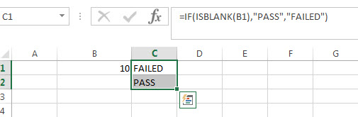
Excel IF function check if the cell is non-blank
If you want to check the value in one cell if it is not blank or not empty cell, then you can use IF function in combination with ISBLANK function or logical operator (not equal to) in excel.
let’s see the generic IF formula with ISBLANK function and Logical operator <> as follows:
=IF(ISBLANK(B1)=FALSE,"PASS","FAILED")
=IF(B1<>"","PASS","FAILED")
In the above two IF formulas, it will return “PASS” if Cell B1 is not blank, otherwise returns “FAILED”.
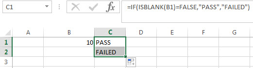
Let’s write a nested if function in combining with AND function and ISBLANK function to achieve the following test criteria.
IF cell A1 is greater than or equal to 10, then add to C1.
If Cell B1 is greather than or equal to 10, then subtract from C1.
If both A1 and b1 are blank cells, then equals to C1.
Based on the above logic, we can write down the following excel nested if formula (statement):
=IF(A1>=0,C1+A1, IF(B1>=0,C1-B1, IF(AND(ISBLANK(A1)=TRUE, ISBLANK(B1)=TRUE),C1,"")))
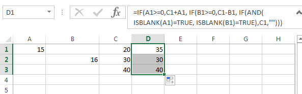
- Excel IF formula with operator : greater than,less than
Now we can use the above logical test with greater than operator. Let’s see the below generic if formula with greater than operator:=IF(A1>10,”excelhow.net”,”google”) … -
Excel IF function with text values
If you want to write an IF formula for text values in combining with the below two logical operators in excel, such as: “equal to” or “not equal to”… -
Excel IF Function With Numbers
If you want to check if a cell values is between two values or checking for the range of numbers or multiple values in cells, at this time, we need to use AND or OR logical function in combination with the logical operator and IF function… -
Excel IF function with Dates
If you have a list of dates and then want to compare to these dates with a specified date to check if those dates is greater than or less than that specified date. …
- Excel AND function
The Excel AND function returns TRUE if all of arguments are TRUE, and it returns FALSE if any of arguments are FALSE.The syntax of the AND function is as below:= AND (condition1,[condition2],…) … - Excel IF function
The Excel IF function perform a logical test to return one value if the condition is TRUE and return another value if the condition is FALSE…. - Excel nested if function
The nested IF function is formed by multiple if statements within one Excel if function. This excel nested if statement makes it possible for a single formula to take multiple actions… - Excel ISBLANK function
The Excel ISBLANK function returns TRUE if the value is blank or null.The syntax of the ISBLANK function is as below:= ISBLANK (value)…
If the return cell in an Excel formula is empty, Excel by default returns 0 instead. For example cell A1 is blank and linked to by another cell. But what if you want to show the exact return value – for empty cells as well as 0 as return values? This article introduces three different options for dealing with empty return values.
Option 1: Don’t display zero values
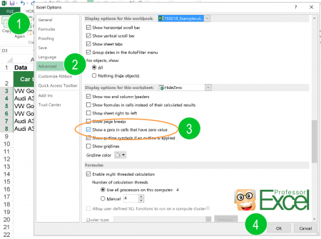
Probably the easiest option is to just not display 0 values. You could differentiate if you want to hide all zeroes from the entire worksheet or just from selected cells.
There are three methods of hiding zero values.
- Hide zero values with conditional formatting rules.
- Blind out zeros with a custom number format.
- Hide zero values within the worksheet settings.
For details about all three methods of just hiding zeroes, please refer to this article.

One small advice on my own account: My Excel add-in “Professor Excel Tools” has a built-in Layout Manager. With this, you can apply this formatting easily to a complete Excel workbook.
Give it a try? Click here and the download starts right away.
Option 2: Change zeroes to blank cells
Unlike the first option, the second option changes the output value. No matter if the return value is 0 (zero) or originally a blank cell, the output of the formula is an empty cell. You can achieve this using the IF formula.

Say, your lookup formula looks like this: =VLOOKUP(A3,C:D,2,FALSE) (hereafter referred to by “original formula”). You want to prevent getting a zero even if the return value―found by the VLOOKUP formula in column D―is an empty value. This can be achieved using the IF formula.
The structure of such IF formula is shown in the image above (if you need assistance with the IF formula, please refer to this article). The original formula is wrapped within the IF formula. The first argument compares if the original formula returns 0. If yes―and that’s the task of the second argument―the formula returns nothing through the double quotation marks. If the orgininal formula within the first argument doesn’t return zero, the last argument returns the real value. This is achieved by the original formula again.
The complete formula looks like this.
=IF(VLOOKUP(A3,C:D,2,FALSE)=0,"",VLOOKUP(A3,C:D,2,FALSE))
Do you want to boost your productivity in Excel?
Get the Professor Excel ribbon!

Add more than 120 great features to Excel!
Option 3: Show zeroes but don’t show blank or empty return values

The previous option two didn’t differentiate between 0 and empty cells in the return cell. If you only want to show empty cells if the return cell found by your lookup formula is empty (and not if the return value really is 0) then you have to slightly alter the formula from option 2 before.
Like before, the IF formula is wrapped around the original formula. But instead of testing if the return value is 0, it tests within the first argument if the return value is blank. This is done by the double quotation marks. The rest of the formula is the as before: With the second argument you define that—if the value from the original formula is blank—the return value is empty too. If not, the last argument defines that you return the desired non-blank value.
The formula in your example from option 2 looks like this.
=IF(VLOOKUP(A3,C:D,2,FALSE)="","",VLOOKUP(A3,C:D,2,FALSE))
Option 4: Use Professor Excel Tools to insert the IF functions very quickly
To save some time, we have included a feature for showing blank cells (instead of zeros) in our Excel add-in Professor Excel Tools.
It’s very simple:
- Select the cells that are supposed to return blanks (instead of zeros).
- Click on the arrow under the “Return Blanks” button on the Professor Excel ribbon and then on either
- Return blanks for zeros and blanks or
- Return zeros for zeros and blanks for blanks.
Professor Excel then inserts the IF function as shown in options 2 and 3 above.

This function is included in our Excel Add-In ‘Professor Excel Tools’
(No sign-up, download starts directly)
Option 5: One elegant solution for not returning zero values…

… was written in the comments. Thanks, Dom! Great to get such awesome feedback from you!
It’s actually quite straight forward: Add two quotation marks in front or after the function and concatenate it with the “&”-character. So, in this case the VLOOKUP function from above would look like this:
=""&VLOOKUP(A3,C:D,2,FALSE)
But: There is a downside. This method forces the cell to a text / string value. This might cause problems in further calculations if a zero is returned. Let me give you an example:
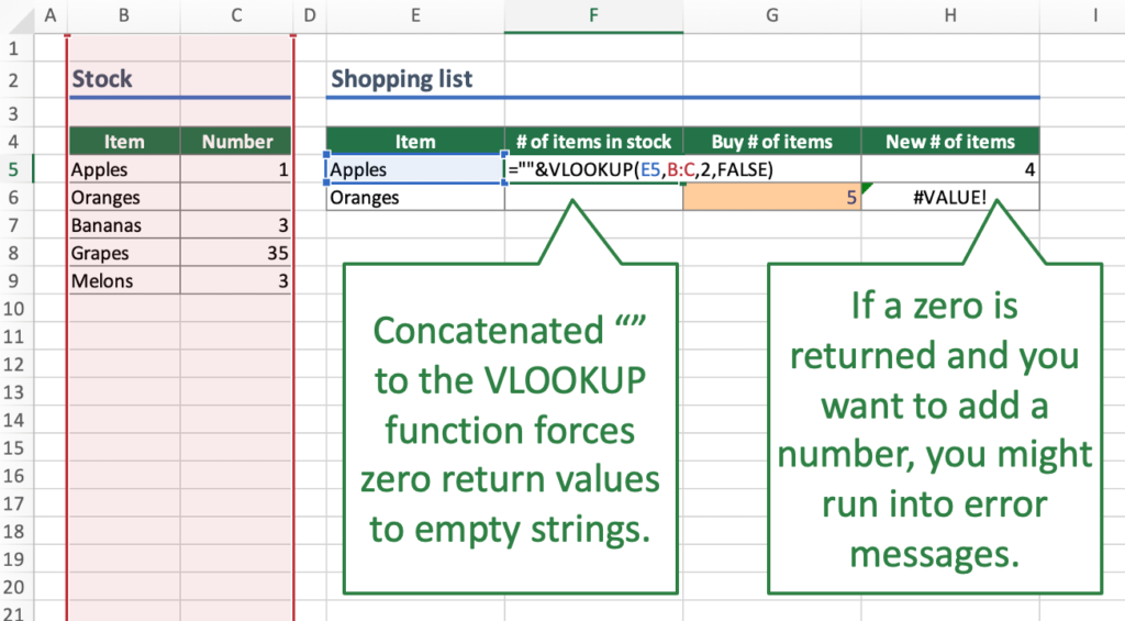
Careful: Return value is interpretated as text.Your VLOOKUP function above is concatenated to an empty string “”. If your return value is 0, the cell will be shown as an empty string. Further calculations might be difficult: For example, if you want to add a number to the return value. Referring directly to the cell, for example =F6+G6 leads to the #VALUE error message as shown above. However, using the SUM function =SUM(F6,G6) still works.
Bottom line: This is an elegant approach, but please test it well if it suits to your Excel model.
Image by Pexels from Pixabay