If and count function in excel

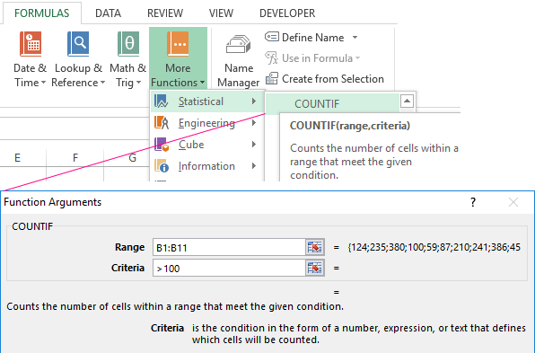
COUNTIF function

Use COUNTIF, one of the statistical functions, to count the number of cells that meet a criterion; for example, to count the number of times a particular city appears in a customer list.

In its simplest form, COUNTIF says:

• =COUNTIF(Where do you want to look?, What do you want to look for?)

For example:

• =COUNTIF(A2:A5,»London»)

• =COUNTIF(A2:A5,A4)

COUNTIF(range, criteria)

Argument name	Description
range    (required)	The group of cells you want to count. Range can contain numbers, arrays, a named range, or references that contain numbers. Blank and text values are ignored. Learn how to select ranges in a worksheet.
criteria    (required)	A number, expression, cell reference, or text string that determines which cells will be counted. For example, you can use a number like 32, a comparison like «>32», a cell like B4, or a word like «apples». COUNTIF uses only a single criteria. Use COUNTIFS if you want to use multiple criteria.

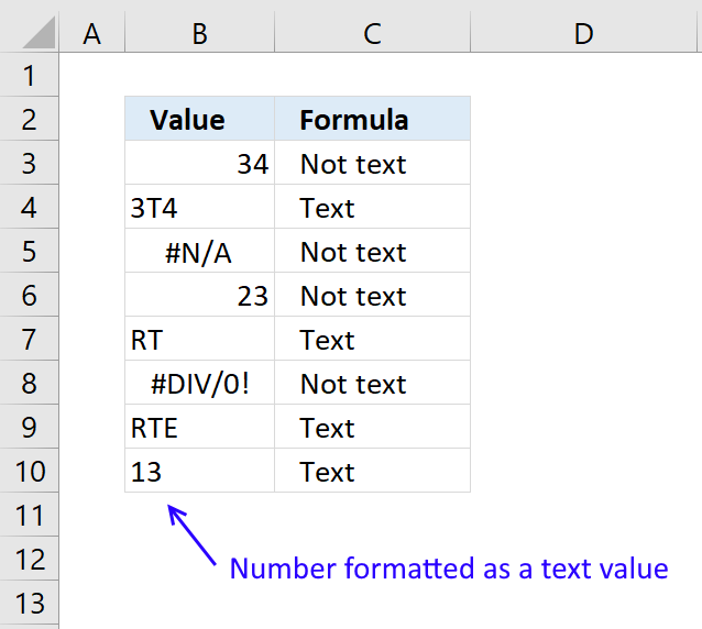
Examples

To use these examples in Excel, copy the data in the table below, and paste it in cell A1 of a new worksheet.

Data	Data
apples	32
oranges	54
peaches	75
apples	86
Formula	Description
=COUNTIF(A2:A5,»apples»)	Counts the number of cells with apples in cells A2 through A5. The result is 2.
=COUNTIF(A2:A5,A4)	Counts the number of cells with peaches (the value in A4) in cells A2 through A5. The result is 1.
=COUNTIF(A2:A5,A2)+COUNTIF(A2:A5,A3)	Counts the number of apples (the value in A2), and oranges (the value in A3) in cells A2 through A5. The result is 3. This formula uses COUNTIF twice to specify multiple criteria, one criteria per expression. You could also use the COUNTIFS function.
=COUNTIF(B2:B5,»>55″)	Counts the number of cells with a value greater than 55 in cells B2 through B5. The result is 2.
=COUNTIF(B2:B5,»<>»&B4)	Counts the number of cells with a value not equal to 75 in cells B2 through B5. The ampersand (&) merges the comparison operator for not equal to (<>) and the value in B4 to read =COUNTIF(B2:B5,»<>75″). The result is 3.
=COUNTIF(B2:B5,»>=32″)-COUNTIF(B2:B5,»<=85″)	Counts the number of cells with a value greater than (>) or equal to (=) 32 and less than (<) or equal to (=) 85 in cells B2 through B5. The result is 1.
=COUNTIF(A2:A5,»*»)	Counts the number of cells containing any text in cells A2 through A5. The asterisk (*) is used as the wildcard character to match any character. The result is 4.
=COUNTIF(A2:A5,»?????es»)	Counts the number of cells that have exactly 7 characters, and end with the letters «es» in cells A2 through A5. The question mark (?) is used as the wildcard character to match individual characters. The result is 2.

Common Problems

Problem	What went wrong
Wrong value returned for long strings.	The COUNTIF function returns incorrect results when you use it to match strings longer than 255 characters. To match strings longer than 255 characters, use the CONCATENATE function or the concatenate operator &. For example, =COUNTIF(A2:A5,»long string»&»another long string»).
No value returned when you expect a value.	Be sure to enclose the criteria argument in quotes.
A COUNTIF formula receives a #VALUE! error when referring to another worksheet.	This error occurs when the formula that contains the function refers to cells or a range in a closed workbook and the cells are calculated. For this feature to work, the other workbook must be open.

Best practices

Do this	Why
Be aware that COUNTIF ignores upper and lower case in text strings.	Criteria aren’t case sensitive. In other words, the string «apples» and the string «APPLES» will match the same cells.
Use wildcard characters.	Wildcard characters —the question mark (?) and asterisk (*)—can be used in criteria. A question mark matches any single character. An asterisk matches any sequence of characters. If you want to find an actual question mark or asterisk, type a tilde (~) in front of the character. For example, =COUNTIF(A2:A5,»apple?») will count all instances of «apple» with a last letter that could vary.
Make sure your data doesn’t contain erroneous characters.	When counting text values, make sure the data doesn’t contain leading spaces, trailing spaces, inconsistent use of straight and curly quotation marks, or nonprinting characters. In these cases, COUNTIF might return an unexpected value. Try using the CLEAN function or the TRIM function.
For convenience, use named ranges	COUNTIF supports named ranges in a formula (such as =COUNTIF(fruit,»>=32″)-COUNTIF(fruit,»>85″). The named range can be in the current worksheet, another worksheet in the same workbook, or from a different workbook. To reference from another workbook, that second workbook also must be open.

Note: The COUNTIF function will not count cells based on cell background or font color. However, Excel supports User-Defined Functions (UDFs) using the Microsoft Visual Basic for Applications (VBA) operations on cells based on background or font color. Here is an example of how you can Count the number of cells with specific cell color by using VBA.

Need more help?

You can always ask an expert in the Excel Tech Community or get support in the Answers community.

See also

COUNTIFS function

IF function

COUNTA function

Overview of formulas in Excel

IFS function

SUMIF function

» » operator surrounded by double quotes («»). For example, the formula below will count cells not equal to «red» in the range A1:A10:

Blank cells

COUNTIF can count cells that are blank or not blank. The formulas below count blank and not blank cells in the range A1:A10:

Note: be aware that COUNTIF treats formulas that return an empty string («») as not blank. See this example for some workarounds to this problem.

Dates

The easiest way to use COUNTIF with dates is to refer to a valid date in another cell with a cell reference. For example, to count cells in A1:A10 that contain a date greater than the date in B1, you can use a formula like this:

Notice we must concatenate an operator to the date in B1. To use more advanced date criteria (i.e. all dates in a given month, or all dates between two dates) you’ll want to switch to the COUNTIFS function, which can handle multiple criteria.

The safest way to hardcode a date into COUNTIF is to use the DATE function. This ensures Excel will understand the date. To count cells in A1:A10 that contain a date less than April 1, 2020, you can use a formula like this

Wildcards

The wildcard characters question mark (?), asterisk(*), or tilde (

) can be used in criteria. A question mark (?) matches any one character and an asterisk (*) matches zero or more characters of any kind. For example, to count cells in A1:A5 that contain the text «apple» anywhere, you can use a formula like this:

To count cells in A1:A5 that contain any 3 text characters, you can use:

) is an escape character to match literal wildcards. For example, to count a literal question mark (?), asterisk(*), or tilde (

), add a tilde in front of the wildcard (i.e.

OR logic

The COUNTIF function is designed to apply just one condition. However, to count cells that contain «this OR that», you can use an array constant and the SUM function like this:

The formula above will count cells in range that contain «red» or «blue». Essentially, COUNTIF returns two counts in an array (one for «red» and one for «blue») and the SUM function returns the sum. For more information, see this example.

Limitations

The COUNTIF function has some limitations you should be aware of:

• COUNTIF only supports a single condition. If you need to count cells using multiple criteria, use the COUNTIFS function.
• COUNTIF requires an actual range for the range argument; you can’t provide an array. This means you can’t alter values in range before applying criteria.
• COUNTIF is not case-sensitive. Use the EXACT function for case-sensitive counts.
• COUNTIFS has other quirks explained in this article.

The most common way to work around the limitations above is to use the SUMPRODUCT function. In the current version of Excel, another option is to use the newer BYROW and BYCOL functions.

Источник

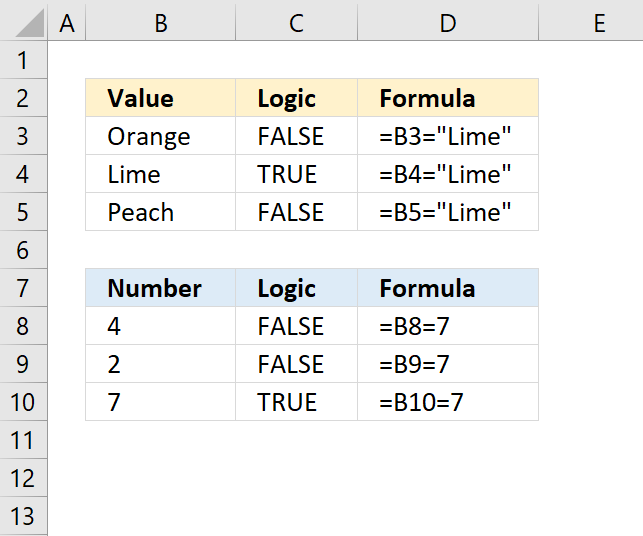
If and count function in excel

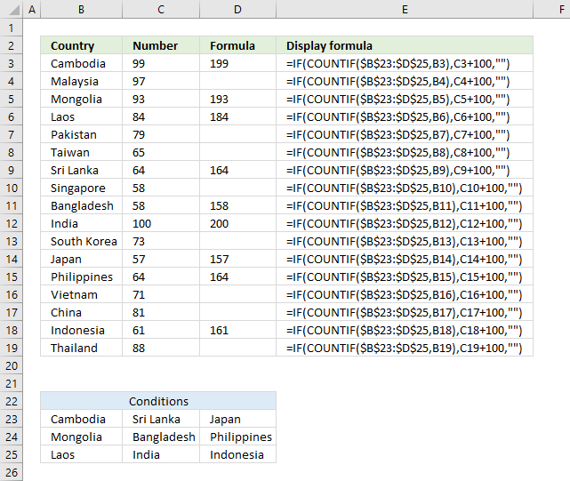
The image above demonstrates a formula that matches a value to multiple conditions, if the condition is met the formula takes the value in a corresponding cell on the same row and adds a given number.

Table of contents

The COUNTIF function allows you to construct a small IF formula that carries out plenty of logical expressions.

Combining the IF and COUNTIF functions also let you have more than 254 logical expressions and the effort to type the formula is minimal.

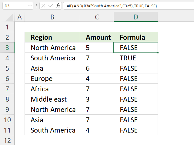
1. Use IF + COUNTIF to evaluate multiple conditions

The example shown in the above picture checks if the country in cell B3 is equal to one of the countries in cell range B23:D25.

In other words, the COUNTIF function counts how many times a specific value is found in a cell range.

If the value exists at least once in the cell range the IF function adds 100 to the value in C3. If FALSE the formula returns a blank.

1.1 Explaining formula in cell D3

Step 1 — COUNTIF function syntax

The COUNTIF function calculates the number of cells that is equal to a condition.

Step 2 — Populate COUNTIF function arguments

range — A reference to all conditions: $B$23:$D$25

criteria — The value to match.

Step 3 — Evaluate COUNTIF function

and returns 1. The criteria value is found once in the array (bolded).

Step 4 — IF function syntax

The IF function returns one value if the logical test is TRUE and another value if the logical test is FALSE.

IF(logical_test, [value_if_true], [value_if_false])

Step 5 — Populate IF function arguments

IF(logical_test, [value_if_true], [value_if_false])

logical_test — True or False, the numerical equivalents are TRUE — 1 and False — 0 (zero). 1, in this case, is equal to TRUE.

[value_if_true] — C3+100, add 100 to value in cell C3.

Step 6 — Evaluate IF function

IF(COUNTIF($B$23:$D$25, B3), C3+100, «»)

and returns 199 in cell D3.

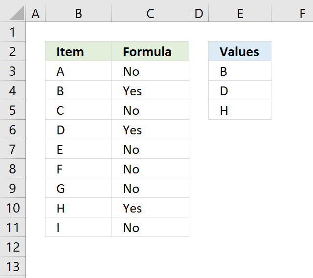
2. Use IF + COUNTIF to evaluate multiple conditions and calculate different outcomes

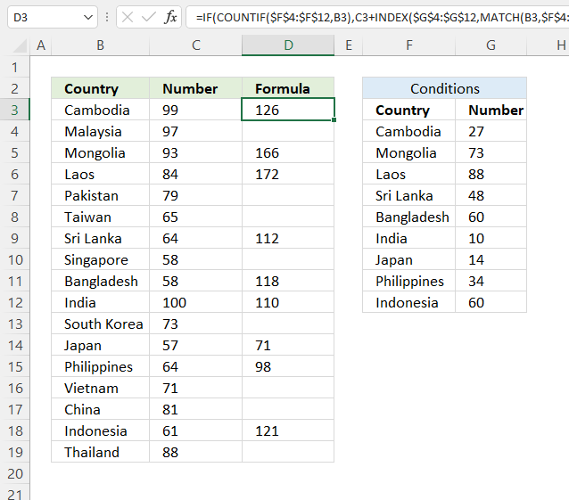
The image above demonstrates a formula in cell D3 that checks if the value in cell B3 matches any of the conditions specified in cell range F4:F12. If so, add the corresponding number in cell range G4:G12 to the number in cell C3.

Formula in cell D3:

2.1 Explaining formula

Step 1 — Check if the value matches any of the conditions

The COUNTIF function calculates the number of cells that is equal to a condition.

and returns 1. This means that there is one value that matches.

Step 2 — IF function

The IF function returns one value if the logical test is TRUE and another value if the logical test is FALSE.

IF(logical_test, [value_if_true], [value_if_false])

IF(COUNTIF($F$4:$F$12, B3), [value_if_true], [value_if_false])

IF(1, [value_if_true], [value_if_false])

[value_if_true] — C3+INDEX($G$4:$G$12, MATCH(B3, $F$4:$F$12,0))

Step 3 — Calculate the relative position of a lookup value

The MATCH function returns the relative position of an item in an array or cell reference that matches a specified value in a specific order.

MATCH(lookup_value, lookup_array, [match_type])

and returns 1. The lookup value is found at the first position in the array.

Step 3 — Get value

The INDEX function returns a value from a cell range, you specify which value based on a row and column number.

INDEX(array, [row_num], [column_num])

INDEX($G$4:$G$12, MATCH(B3, $F$4:$F$12,0))

Step 4 — Add values

The plus sign lets you add numbers in an Excel formula.

C3+INDEX($G$4:$G$12, MATCH(B3, $F$4:$F$12,0))

99 + 27 equals 126.

Get Excel *.xlsx file

Logic category

Functions in this article

Excel formula categories

Excel categories

3 Responses to “Use IF + COUNTIF to evaluate multiple conditions”

1. If item Count in Column-A have equal Count of the same item in corresponding Column-B, Result should be «Complete»
2. If item Count in Column-A have Count at least one in corresponding Column-B but less than Count in Column-A, Result should be «In progress»
3. If item Count in Column-A have no Count in corresponding Column-B, Result should be «Not Complete»
4. If there is no Count in Column-A and corresponding Column-B have no count, Result should be «Blank»

Please reply
If the marks of a student is less than 16 or his average is less than 50 he must be in D group.
How can i write this formula? Please write it for me

Please reply
If the marks of a student is less than 16 or his average is less than 50 he must be in D group.
How can i write this formula in table of contant? Please write it for me

Leave a Reply

How to comment

How to add a formula to your comment
Insert your formula here.

Convert less than and larger than signs
Use html character entities instead of less than and larger than signs.
becomes >

How to add VBA code to your comment
[vb 1=»vbnet» language=»,»]
Put your VBA code here.
[/vb]

How to add a picture to your comment:
Upload picture to postimage.org or imgur
Paste image link to your comment.

Contact Oscar

You can contact me through this contact form

Источник

COUNTIF function

Use COUNTIF, one of the statistical functions, to count the number of cells that meet a criterion; for example, to count the number of times a particular city appears in a customer list.

In its simplest form, COUNTIF says:

=COUNTIF(Where do you want to look?, What do you want to look for?)

The group of cells you want to count. Range can contain numbers, arrays, a named range, or references that contain numbers. Blank and text values are ignored.

A number, expression, cell reference, or text string that determines which cells will be counted.

For example, you can use a number like 32, a comparison like «>32», a cell like B4, or a word like «apples».

COUNTIF uses only a single criteria. Use COUNTIFS if you want to use multiple criteria.

Examples

To use these examples in Excel, copy the data in the table below, and paste it in cell A1 of a new worksheet.

Counts the number of cells with apples in cells A2 through A5. The result is 2.

Counts the number of cells with peaches (the value in A4) in cells A2 through A5. The result is 1.

Counts the number of apples (the value in A2), and oranges (the value in A3) in cells A2 through A5. The result is 3. This formula uses COUNTIF twice to specify multiple criteria, one criteria per expression. You could also use the COUNTIFS function.

Counts the number of cells with a value greater than 55 in cells B2 through B5. The result is 2.

Counts the number of cells with a value not equal to 75 in cells B2 through B5. The ampersand (&) merges the comparison operator for not equal to (<>) and the value in B4 to read =COUNTIF(B2:B5,»<>75″). The result is 3.

=COUNTIF(B2:B5,»>=32″)-COUNTIF(B2:B5,» ) or equal to (=) 32 and less than (

Common Problems

What went wrong

Wrong value returned for long strings.

The COUNTIF function returns incorrect results when you use it to match strings longer than 255 characters.

To match strings longer than 255 characters, use the CONCATENATE function or the concatenate operator &. For example, =COUNTIF(A2:A5,»long string»&»another long string»).

No value returned when you expect a value.

Be sure to enclose the criteria argument in quotes.

A COUNTIF formula receives a #VALUE! error when referring to another worksheet.

This error occurs when the formula that contains the function refers to cells or a range in a closed workbook and the cells are calculated. For this feature to work, the other workbook must be open.

Best practices

Be aware that COUNTIF ignores upper and lower case in text strings.

Criteria aren’t case sensitive. In other words, the string «apples» and the string «APPLES» will match the same cells.

Use wildcard characters.

Wildcard characters —the question mark (?) and asterisk (*)—can be used in criteria. A question mark matches any single character. An asterisk matches any sequence of characters. If you want to find an actual question mark or asterisk, type a tilde (

) in front of the character.

For example, =COUNTIF(A2:A5,»apple?») will count all instances of «apple» with a last letter that could vary.

Make sure your data doesn’t contain erroneous characters.

When counting text values, make sure the data doesn’t contain leading spaces, trailing spaces, inconsistent use of straight and curly quotation marks, or nonprinting characters. In these cases, COUNTIF might return an unexpected value.

For convenience, use named ranges

COUNTIF supports named ranges in a formula (such as =COUNTIF( fruit,»>=32″)-COUNTIF( fruit,»>85″). The named range can be in the current worksheet, another worksheet in the same workbook, or from a different workbook. To reference from another workbook, that second workbook also must be open.

Note: The COUNTIF function will not count cells based on cell background or font color. However, Excel supports User-Defined Functions (UDFs) using the Microsoft Visual Basic for Applications (VBA) operations on cells based on background or font color. Here is an example of how you can Count the number of cells with specific cell color by using VBA.

Need more help?

You can always ask an expert in the Excel Tech Community or get support in the Answers community.

Источник

Adblock
detector

The COUNTIF function counts cells in a range that meet a given condition, referred to as criteria. COUNTIF is a common, widely used function in Excel, and can be used to count cells that contain dates, numbers, and text. Note that COUNTIF can only apply a single condition. To count cells with multiple criteria, see the COUNTIFS function.

Syntax

The generic syntax for COUNTIF looks like this:

=COUNTIF(range,criteria)

The COUNTIF function takes two arguments, range and criteria. Range is the range of cells to apply a condition to. Criteria is the condition to apply, along with any logical operators that are needed.

Applying criteria

The COUNTIF function supports logical operators (>,<,<>,<=,>=) and wildcards (*,?) for partial matching. The tricky part about using the COUNTIF function is the syntax used to apply criteria. COUNTIFS is in a group of eight functions that split logical criteria into two parts, range and criteria. Because of this design, each condition requires a separate range and criteria argument, and operators in the criteria must be enclosed in double quotes («»). The table below shows examples of the syntax needed for common criteria:

Target	Criteria
Cells greater than 75	«>75»
Cells equal to 100	100 or «100»
Cells less than or equal to 100	«<=100»
Cells equal to «Red»	«red»
Cells not equal to «Red»	«<>red»
Cells that are blank «»	«»
Cells that are not blank	«<>»
Cells that begin with «X»	«x*»
Cells less than A1	«<«&A1
Cells less than today	«<«&TODAY()

Notice the last two examples involve concatenation with the ampersand (&) character.  Any time you are using a value from another cell, or using the result of a formula in criteria with a logical operator like «<«, you will need to concatenate. This is because Excel needs to evaluate cell references and formulas first to get a value, before that value can be joined to an operator.

Basic example

In the worksheet shown above, the following formulas are used in cells G5, G6, and G7:

=COUNTIF(D5:D12,">100") // count sales over 100
=COUNTIF(B5:B12,"jim") // count name = "jim"
=COUNTIF(C5:C12,"ca") // count state = "ca"

Notice COUNTIF is not case-sensitive, «CA» and «ca» are treated the same.

Double quotes («») in criteria

In general, text values need to be enclosed in double quotes («»), and numbers do not. However, when a logical operator is included with a number, the number and operator must be enclosed in quotes, as seen in the second example below:

=COUNTIF(A1:A10,100) // count cells equal to 100
=COUNTIF(A1:A10,">32") // count cells greater than 32
=COUNTIF(A1:A10,"jim") // count cells equal to "jim"

Value from another cell

A value from another cell can be included in criteria using concatenation. In the example below, COUNTIF will return the count of values in A1:A10 that are less than the value in cell B1. Notice the less than operator (which is text) is enclosed in quotes.

=COUNTIF(A1:A10,"<"&B1) // count cells less than  B1

Not equal to

To construct «not equal to» criteria, use the «<>» operator surrounded by double quotes («»). For example, the formula below will count cells not equal to «red» in the range A1:A10:

=COUNTIF(A1:A10,"<>red") // not "red"

Blank cells

COUNTIF can count cells that are blank or not blank. The formulas below count blank and not blank cells in the range A1:A10:

=COUNTIF(A1:A10,"<>") // not blank
=COUNTIF(A1:A10,"") // blank

Note: be aware that COUNTIF treats formulas that return an empty string («») as not blank. See this example for some workarounds to this problem.

Dates

The easiest way to use COUNTIF with dates is to refer to a valid date in another cell with a cell reference. For example, to count cells in A1:A10 that contain a date greater than the date in B1, you can use a formula like this:

=COUNTIF(A1:A10, ">"&B1) // count dates greater than A1

Notice we must concatenate an operator to the date in B1. To use more advanced date criteria (i.e. all dates in a given month, or all dates between two dates) you’ll want to switch to the COUNTIFS function, which can handle multiple criteria.

The safest way to hardcode a date into COUNTIF is to use the DATE function. This ensures Excel will understand the date. To count cells in A1:A10 that contain a date less than April 1, 2020, you can use a formula like this

=COUNTIF(A1:A10,"<"&DATE(2020,4,1)) // dates less than 1-Apr-2020

Wildcards

The wildcard characters question mark (?), asterisk(*), or tilde (~) can be used in criteria. A question mark (?) matches any one character and an asterisk (*) matches zero or more characters of any kind. For example, to count cells in A1:A5 that contain the text «apple» anywhere, you can use a formula like this:

=COUNTIF(A1:A5,"*apple*") // cells that contain "apple"

To count cells in A1:A5 that contain any 3 text characters, you can use:

=COUNTIF(A1:A5,"???") // cells that contain any 3 characters

The tilde (~) is an escape character to match literal wildcards. For example, to count a literal question mark (?), asterisk(*), or tilde (~), add a tilde in front of the wildcard (i.e. ~?, ~*, ~~).

OR logic

The COUNTIF function is designed to apply just one condition. However, to count cells that contain «this OR that», you can use an array constant and the SUM function like this:

=SUM(COUNTIF(range,{"red","blue"})) // red or blue

The formula above will count cells in range that contain «red» or «blue». Essentially, COUNTIF returns two counts in an array (one for «red» and one for «blue») and the SUM function returns the sum. For more information, see this example.

Limitations

The COUNTIF function has some limitations you should be aware of:

• COUNTIF only supports a single condition. If you need to count cells using multiple criteria, use the COUNTIFS function.
• COUNTIF requires an actual range for the range argument; you can’t provide an array. This means you can’t alter values in range before applying criteria.
• COUNTIF is not case-sensitive. Use the EXACT function for case-sensitive counts.
• COUNTIFS has other quirks explained in this article.

The most common way to work around the limitations above is to use the SUMPRODUCT function. In the current version of Excel, another option is to use the newer BYROW and BYCOL functions.

Notes

• Text strings in criteria must be enclosed in double quotes («»), i.e. «apple», «>32», «app*»
• Cell references in criteria are not enclosed in quotes, i.e. «<«&A1
• The wildcard characters ? and * can be used in criteria. A question mark matches any one character and an asterisk matches any sequence of characters (zero or more).
• To match a literal question mark(?) or asterisk (*), use a tilde (~) like (~?, ~*).
• COUNTIF requires a range, you can’t substitute an array.
• COUNTIF returns incorrect results when used to match strings longer than 255 characters.
• COUNTIF will return a #VALUE error when referencing another workbook that is closed.

Author: Oscar Cronquist Article last updated on September 17, 2021

The image above demonstrates a formula that matches a value to multiple conditions, if the condition is met the formula takes the value in a corresponding cell on the same row and adds a given number.

The COUNTIF function allows you to construct a small IF formula that carries out plenty of logical expressions.

Combining the IF and COUNTIF functions also let you have more than 254 logical expressions and the effort to type the formula is minimal.

1. Use IF + COUNTIF to evaluate multiple conditions

=IF(COUNTIF($B$23:$D$25,B3),C3+100,»»)

The example shown in the above picture checks if the country in cell B3 is equal to one of the countries in cell range B23:D25.

In other words, the COUNTIF function counts how many times a specific value is found in a cell range.

If the value exists at least once in the cell range the IF function adds 100 to the value in C3. If FALSE the formula returns a blank.

Back to top

1.1 Explaining formula in cell D3

Step 1 — COUNTIF function syntax

The COUNTIF function calculates the number of cells that is equal to a condition.

COUNTIF(range, criteria)

Step 2 — Populate COUNTIF function arguments

COUNTIF(range, criteria)

becomes

COUNTIF($B$23:$D$25,B3)

range — A reference to all conditions: $B$23:$D$25

criteria — The value to match.

Step 3 — Evaluate COUNTIF function

COUNTIF($B$23:$D$25,B3)

becomes

COUNTIF({«Cambodia«, «Sri Lanka», «Japan»; «Mongolia», «Bangladesh», «Philippines»; «Laos», «India», «Indonesia»}, «Cambodia«)

and returns 1. The criteria value is found once in the array (bolded).

Step 4 — IF function syntax

The IF function returns one value if the logical test is TRUE and another value if the logical test is FALSE.

IF(logical_test, [value_if_true], [value_if_false])

Step 5 — Populate IF function arguments

IF(logical_test, [value_if_true], [value_if_false])

becomes

IF(1, C3+100, «»)

logical_test — True or False, the numerical equivalents are TRUE — 1 and False — 0 (zero). 1, in this case, is equal to TRUE.

[value_if_true] — C3+100, add 100 to value in cell C3.

[value_if_false] — «».

Step 6 — Evaluate IF function

IF(COUNTIF($B$23:$D$25, B3), C3+100, «»)

becomes

IF(1, C3+100, «»)

becomes

C3 + 100

becomes

99 + 100

and returns 199 in cell D3.

Back to top

2. Use IF + COUNTIF to evaluate multiple conditions and calculate different outcomes

The image above demonstrates a formula in cell D3 that checks if the value in cell B3 matches any of the conditions specified in cell range F4:F12. If so, add the corresponding number in cell range G4:G12 to the number in cell C3.

Formula in cell D3:

=IF(COUNTIF($F$4:$F$12, B3), C3+INDEX($G$4:$G$12, MATCH(B3, $F$4:$F$12,0)), «»)

Back to top

2.1 Explaining formula

Step 1 — Check if the value matches any of the conditions

The COUNTIF function calculates the number of cells that is equal to a condition.

COUNTIF(range, criteria)

COUNTIF($F$4:$F$12, B3)

becomes

COUNTIF({«Cambodia«; «Mongolia»; «Laos»; «Sri Lanka»; «Bangladesh»; «India»; «Japan»; «Philippines»; «Indonesia»}, «Cambodia«)

and returns 1. This means that there is one value that matches.

Step 2 — IF function

The IF function returns one value if the logical test is TRUE and another value if the logical test is FALSE.

IF(logical_test, [value_if_true], [value_if_false])

IF(COUNTIF($F$4:$F$12, B3), [value_if_true], [value_if_false])

becomes

IF(1, [value_if_true], [value_if_false])

[value_if_true] — C3+INDEX($G$4:$G$12, MATCH(B3, $F$4:$F$12,0))

[value_if_false] — «»

Step 3 — Calculate the relative position of a lookup value

The MATCH function returns the relative position of an item in an array or cell reference that matches a specified value in a specific order.

MATCH(lookup_value, lookup_array, [match_type])

MATCH(B3, $F$4:$F$12,0)

becomes

MATCH(«Cambodia», {«Cambodia»; «Mongolia»; «Laos»; «Sri Lanka»; «Bangladesh»; «India»; «Japan»; «Philippines»; «Indonesia»}, 0)

and returns 1. The lookup value is found at the first position in the array.

Step 3 — Get value

The INDEX function returns a value from a cell range, you specify which value based on a row and column number.

INDEX(array, [row_num], [column_num])

INDEX($G$4:$G$12, MATCH(B3, $F$4:$F$12,0))

becomes

INDEX($G$4:$G$12, 1)

and returns 27.

Step 4 — Add values

The plus sign lets you add numbers in an Excel formula.

C3+INDEX($G$4:$G$12, MATCH(B3, $F$4:$F$12,0))

becomes

99 + 27 equals 126.

Back to top

Get Excel *.xlsx file

Use IF + COUNTIF to perform multiple conditionsv2

Back to top

Excel has many functions where a user needs to specify a single or multiple criteria to get the result. For example, if you want to count cells based on multiple criteria, you can use the COUNTIF or COUNTIFS functions in Excel.

This tutorial covers various ways of using a single or multiple criteria in COUNTIF and COUNTIFS function in Excel.

While I will primarily be focussing on COUNTIF and COUNTIFS functions in this tutorial, all these examples can also be used in other Excel functions that take multiple criteria as inputs (such as SUMIF, SUMIFS, AVERAGEIF, and AVERAGEIFS).

An Introduction to Excel COUNTIF and COUNTIFS Functions

Let’s first get a grip on using COUNTIF and COUNTIFS functions in Excel.

Excel COUNTIF Function (takes Single Criteria)

Excel COUNTIF function is best suited for situations when you want to count cells based on a single criterion. If you want to count based on multiple criteria, use COUNTIFS function.

Syntax

=COUNTIF(range, criteria)

Input Arguments

• range –  the range of cells which you want to count.
• criteria – the criteria that must be evaluated against the range of cells for a cell to be counted.

Excel COUNTIFS Function (takes Multiple Criteria)

Excel COUNTIFS function is best suited for situations when you want to count cells based on multiple criteria.

Syntax

=COUNTIFS(criteria_range1, criteria1, [criteria_range2, criteria2]…)

Input Arguments

• criteria_range1 – The range of cells for which you want to evaluate against criteria1.
• criteria1 – the criteria which you want to evaluate for criteria_range1 to determine which cells to count.
• [criteria_range2] – The range of cells for which you want to evaluate against criteria2.
• [criteria2] – the criteria which you want to evaluate for criteria_range2 to determine which cells to count.

Now let’s have a look at some examples of using multiple criteria in COUNTIF functions in Excel.

Using NUMBER Criteria in Excel COUNTIF Functions

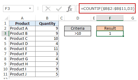
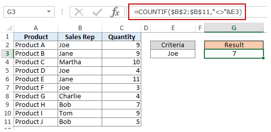
#1 Count Cells when Criteria is EQUAL to a Value

To get the count of cells where the criteria argument is equal to a specified value, you can either directly enter the criteria or use the cell reference that contains the criteria.

Below is an example where we count the cells that contain the number 9 (which means that the criteria argument is equal to 9). Here is the formula:

=COUNTIF($B$2:$B$11,D3)

In the above example (in the pic), the criteria is in cell D3. You can also enter the criteria directly into the formula. For example, you can also use:

=COUNTIF($B$2:$B$11,9)

#2 Count Cells when Criteria is GREATER THAN a Value

To get the count of cells with a value greater than a specified value, we use the greater than operator (“>”). We could either use it directly in the formula or use a cell reference that has the criteria.

Whenever we use an operator in criteria in Excel, we need to put it within double quotes. For example, if the criteria is greater than 10, then we need to enter “>10” as the criteria (see pic below):

Here is the formula:

=COUNTIF($B$2:$B$11,”>10″)

You can also have the criteria in a cell and use the cell reference as the criteria. In this case, you need NOT put the criteria in double quotes:

=COUNTIF($B$2:$B$11,D3)

There could also be a case when you want the criteria to be in a cell, but don’t want it with the operator. For example, you may want the cell D3 to have the number 10 and not >10.

In that case, you need to create a criteria argument which is a combination of operator and cell reference (see pic below):

=COUNTIF($B$2:$B$11,”>”&D3)

NOTE: When you combine an operator and a cell reference, the operator is always in double quotes. The operator and cell reference are joined by an ampersand (&).

#3 Count Cells when Criteria is LESS THAN a Value

To get the count of cells with a value less than a specified value, we use the less than operator (“<“). We could either use it directly in the formula or use a cell reference that has the criteria.

Whenever we use an operator in criteria in Excel, we need to put it within double quotes. For example, if the criterion is that the number should be less than 5, then we need to enter “<5” as the criteria (see pic below):

=COUNTIF($B$2:$B$11,”<5″)

You can also have the criteria in a cell and use the cell reference as the criteria. In this case, you need NOT put the criteria in double quotes (see pic below):

=COUNTIF($B$2:$B$11,D3)

Also, there could be a case when you want the criteria to be in a cell, but don’t want it with the operator. For example, you may want the cell D3 to have the number 5 and not <5.

In that case, you need to create a criteria argument which is a combination of operator and cell reference:

=COUNTIF($B$2:$B$11,”<“&D3)

NOTE: When you combine an operator and a cell reference, the operator is always in double quotes. The operator and cell reference are joined by an ampersand (&).

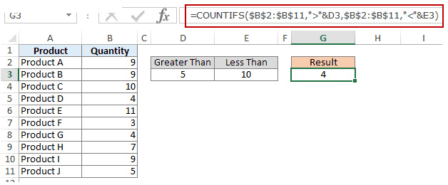
#4 Count Cells with Multiple Criteria – Between Two Values

To get a count of values between two values, we need to use multiple criteria in the COUNTIF function.

Here are two methods of doing this:

METHOD 1: Using COUNTIFS function

COUNTIFS function can handle multiple criteria as arguments and counts the cells only when all the criteria are TRUE. To count cells with values between two specified values (say 5 and 10), we can use the following COUNTIFS function:

=COUNTIFS($B$2:$B$11,”>5″,$B$2:$B$11,”<10″)

NOTE: The above formula does not count cells that contain 5 or 10. If you want to include these cells, use greater than equal to (>=) and less than equal to (<=) operators. Here is the formula:

=COUNTIFS($B$2:$B$11,”>=5″,$B$2:$B$11,”<=10″) 

You can also have these criteria in cells and use the cell reference as the criteria. In this case, you need NOT put the criteria in double quotes (see pic below):

You can also use a combination of cells references and operators (where the operator is entered directly in the formula). When you combine an operator and a cell reference, the operator is always in double quotes. The operator and cell reference are joined by an ampersand (&).

METHOD 2: Using two COUNTIF functions

If you have multiple criteria, you can either use COUNTIFS or create a combination of COUNTIF functions. The formula below would also do the same thing:

=COUNTIF($B$2:$B$11,”>5″)-COUNTIF($B$2:$B$11,”>10″)

In the above formula, we first find the number of cells that have a value greater than 5 and we subtract the count of cells with a value greater than 10. This would give us the result as 5 (which is the number of cells that have values more than 5 and less than equal to 10).

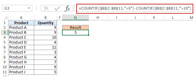
If you want the formula to include both 5 and 10, use the following formula instead:

=COUNTIF($B$2:$B$11,”>=5″)-COUNTIF($B$2:$B$11,”>10″)

If you want the formula to exclude both ‘5’ and ’10’ from the counting, use the following formula:

=COUNTIF($B$2:$B$11,”>=5″)-COUNTIF($B$2:$B$11,”>10″)-COUNTIF($B$2:$B$11,10)

You can have these criteria in cells and use the cells references, or you can use a combination of operators and cells references.

Using TEXT Criteria in Excel Functions

#1 Count Cells when Criteria is EQUAL to a Specified text

To count cells that contain an exact match of the specified text, we can simply use that text as the criteria. For example, in the dataset (shown below in the pic), if I want to count all the cells with the name Joe in it, I can use the below formula:

=COUNTIF($B$2:$B$11,”Joe”)

Since this is a text string, I need to put the text criteria in double quotes.

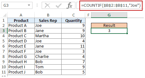
You can also have the criteria in a cell and then use that cell reference (as shown below):

=COUNTIF($B$2:$B$11,E3)

NOTE: You can get wrong results if there are leading/trailing spaces in the criteria or criteria range. Make sure you clean the data before using these formulas.

#2 Count Cells when Criteria is NOT EQUAL to a Specified text

Similar to what we saw in the above example, you can also count cells that do not contain a specified text. To do this, we need to use the not equal to operator (<>).

Suppose you want to count all the cells that do not contain the name JOE, here is the formula that will do it:

=COUNTIF($B$2:$B$11,”<>Joe”)

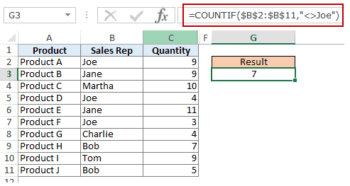
You can also have the criteria in a cell and use the cell reference as the criteria. In this case, you need NOT put the criteria in double quotes (see pic below):

=COUNTIF($B$2:$B$11,E3)

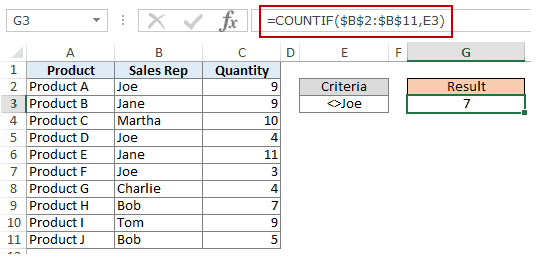
There could also be a case when you want the criteria to be in a cell but don’t want it with the operator. For example, you may want the cell D3 to have the name Joe and not <>Joe.

In that case, you need to create a criteria argument which is a combination of operator and cell reference (see pic below):

=COUNTIF($B$2:$B$11,”<>”&E3)

When you combine an operator and a cell reference, the operator is always in double quotes. The operator and cell reference are joined by an ampersand (&).

Using DATE Criteria in Excel COUNTIF and COUNTIFS Functions

Excel store date and time as numbers. So we can use it the same way we use numbers.

#1 Count Cells when Criteria is EQUAL to a Specified Date

To get the count of cells that contain the specified date, we would use the equal to operator (=) along with the date.

To use the date, I recommend using the DATE function, as it gets rid of any possibility of error in the date value. So, for example, if I want to use the date September 1, 2015, I can use the DATE function as shown below:

=DATE(2015,9,1)

This formula would return the same date despite regional differences. For example, 01-09-2015 would be September 1, 2015 according to the  US date syntax and January 09, 2015 according to the UK date syntax. However, this formula would always return September 1, 2105.

Here is the formula to count the number of cells that contain the date 02-09-2015:

=COUNTIF($A$2:$A$11,DATE(2015,9,2))

#2 Count Cells when Criteria is BEFORE or AFTER to a Specified Date

To count cells that contain date before or after a specified date, we can use the less than/greater than operators.

For example, if I want to count all the cells that contain a date that is after September 02, 2015, I can use the formula:

=COUNTIF($A$2:$A$11,”>”&DATE(2015,9,2))

Similarly, you can also count the number of cells before a specified date. If you want to include a date in the counting, use and ‘equal to’ operator along with ‘greater than/less than’ operator.

You can also use a cell reference that contains a date. In this case, you need to combine the operator (within double quotes) with the date using an ampersand (&).

See example below:

=COUNTIF($A$2:$A$11,”>”&F3)

#3 Count Cells with Multiple Criteria – Between Two Dates

To get a count of values between two values, we need to use multiple criteria in the COUNTIF function.

We can do this using two methods – One single COUNTIFS function or two COUNTIF functions.

METHOD 1: Using COUNTIFS function

COUNTIFS function can take multiple criteria as the arguments and counts the cells only when all the criteria are TRUE. To count cells with values between two specified dates (say September 2 and September 7), we can use the following COUNTIFS function:

=COUNTIFS($A$2:$A$11,”>”&DATE(2015,9,2),$A$2:$A$11,”<“&DATE(2015,9,7))

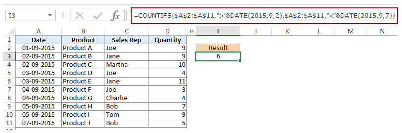
The above formula does not count cells that contain the specified dates. If you want to include these dates as well, use greater than equal to (>=) and less than equal to (<=) operators. Here is the formula:

=COUNTIFS($A$2:$A$11,”>=”&DATE(2015,9,2),$A$2:$A$11,”<=”&DATE(2015,9,7))

You can also have the dates in a cell and use the cell reference as the criteria. In this case, you can not have the operator with the date in the cells. You need to manually add operators in the formula (in double quotes) and add cell reference using an ampersand (&). See the pic below:

=COUNTIFS($A$2:$A$11,”>”&F3,$A$2:$A$11,”<“&G3)

METHOD 2: Using COUNTIF functions

If you have multiple criteria, you can either use one COUNTIFS function or create a combination of two COUNTIF functions. The formula below would also do the trick:

=COUNTIF($A$2:$A$11,”>”&DATE(2015,9,2))-COUNTIF($A$2:$A$11,”>”&DATE(2015,9,7))

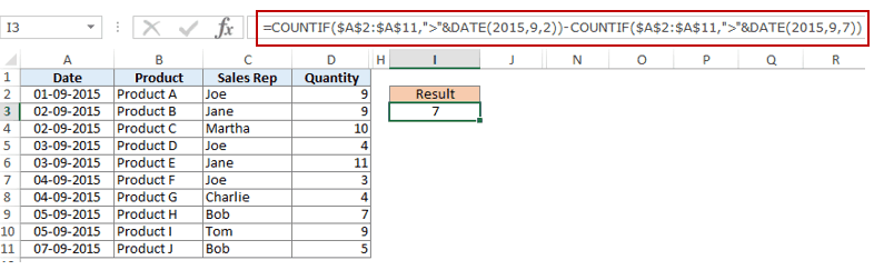
In the above formula, we first find the number of cells that have a date after September 2 and we subtract the count of cells with dates after September 7. This would give us the result as 7 (which is the number of cells that have dates after September 2 and on or before September 7).

If you don’t want the formula to count both September 2 and September 7, use the following formula instead:

=COUNTIF($A$2:$A$11,”>=”&DATE(2015,9,2))-COUNTIF($A$2:$A$11,”>”&DATE(2015,9,7))

If you want to exclude both the dates from counting, use the following formula:

=COUNTIF($A$2:$A$11,”>”&DATE(2015,9,2))-COUNTIF($A$2:$A$11,”>”&DATE(2015,9,7)-COUNTIF($A$2:$A$11,DATE(2015,9,7)))

Also, you can have the criteria dates in cells and use the cells references (along with operators in double quotes joined using ampersand).

Using WILDCARD CHARACTERS in Criteria in COUNTIF & COUNTIFS Functions

There are three wildcard characters in Excel:

1. * (asterisk) – It represents any number of characters. For example, ex* could mean excel, excels, example, expert, etc.
2. ? (question mark) – It represents one single character. For example, Tr?mp could mean Trump or Tramp.
3. ~ (tilde) – It is used to identify a wildcard character (~, *, ?) in the text.

You can use COUNTIF function with wildcard characters to count cells when other inbuilt count function fails. For example, suppose you have a data set as shown below:

Now let’s take various examples:

#1 Count Cells that contain Text

To count cells with text in it, we can use the wildcard character * (asterisk). Since asterisk represents any number of characters, it would count all cells that have any text in it. Here is the formula:

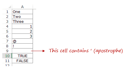
=COUNTIFS($C$2:$C$11,”*”)

Note: The formula above ignores cells that contain numbers, blank cells, and logical values, but would count the cells contain an apostrophe (and hence appear blank) or cells that contain empty string (=””) which may have been returned as a part of a formula.

Here is a detailed tutorial on handling cases where there is an empty string or apostrophe.

Here is a detailed tutorial on handling cases where there are empty strings or apostrophes.

Below is a video that explains different scenarios of counting cells with text in it.

#2 Count Non-blank Cells

If you are thinking of using COUNTA function, think again.

Try it and it might fail you. COUNTA will also count a cell that contains an empty string (often returned by formulas as =”” or when people enter only an apostrophe in a cell). Cells that contain empty strings look blank but are not, and thus counted by the COUNTA function.

COUNTA will also count a cell that contains an empty string (often returned by formulas as =”” or when people enter only an apostrophe in a cell). Cells that contain empty strings look blank but are not, and thus counted by the COUNTA function.

So if you use the formula =COUNTA(A1:A11), it returns 11, while it should return 10.

Here is the fix:

=COUNTIF($A$1:$A$11,”?*”)+COUNT($A$1:$A$11)+SUMPRODUCT(–ISLOGICAL($A$1:$A$11))

Let’s understand this formula by breaking it down:

#3 Count Cells that contain specific text

Let’s say we want to count all the cells where the sales rep name begins with J. This can easily be achieved by using a wildcard character in COUNTIF function. Here is the formula:

=COUNTIFS($C$2:$C$11,”J*”) 

The criteria J* specifies that the text in a cell should begin with J and can contain any number of characters.

If you want to count cells that contain the alphabet anywhere in the text, flank it with an asterisk on both sides. For example, if you want to count cells that contain the alphabet “a” in it, use *a* as the criteria.

This article is unusually long compared to my other articles. Hope you have enjoyed it. Let me know your thoughts by leaving a comment.

You May Also Find the following Excel tutorials useful:

• Count the number of words in Excel.
• Count Cells Based on Background Color in Excel.
• How to Sum a Column in Excel (5 Really Easy Ways)

The COUNTIF function is included in the group of statistical functions. It allows you to find the number of cells by a certain criterion. The COUNTIF function works with numeric and text values, as well as with dates.



Syntax and features of the function

First, let’s consider the arguments:

• Range – the group of values for analysis and counting (required).
• Criteria – the condition by which cells are to be counted (required).

The range of cells can include textual and numerical values, dates, arrays, and references to numbers. The function ignores empty cells.

A criterion can be a reference, a number, a text string, or an expression. The COUNTIF function only works with one criterion (by default). However, you can “force” it to analyze two criteria simultaneously.

Recommendations for the correct operation of the function:

1. If the COUNTIF function refers to a range in another workbook, this workbook must be opened.
2. The «Criteria» argument must be enclosed in quotation marks (except for references).
3. The function does not take into account the letter case.
4. When formulating a counting condition, you can use wildcard characters. The question mark «?» is any character. The asterisk «*» is any sequence of characters. For the formula to search for these signs directly, put a tilde (~) before them.
5. For normal operation of the formula, cells with text values should not contain spaces or non-printable characters.



Countif function in Excel: examples

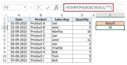
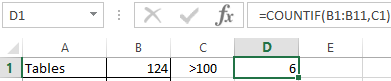
Let’s count the numerical values in one range. The counting condition is one criterion.

We have the following table:

Count the number of cells with numbers greater than 100. Formula: =COUNTIF(B1:B11,»>100″). The range is В1:В11. The counting criterion is «>100». The result:

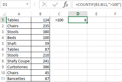
If the counting condition is entered in a separate cell, you can use the reference as a criterion:

Count the text values in one range. The search condition is one criterion. Formula: =COUNTIF(A1:A11,A3).

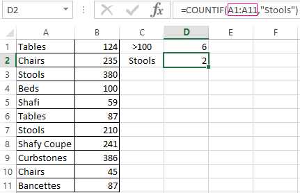
Or used reference inside the table:

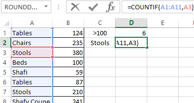
In the second case, the cell reference was used as a criterion, result is the same – 2.

Formula with the wildcard character application: =COUNTIF(A1:A11,»Tab*»). To calculate the number of values ending in «и» and containing any number of characters: =COUNTIF(A1:A11,»*s»). We obtain:

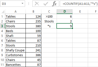
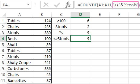
All names that end with a letter «s».

We use the search condition «not equal» in the COUNTIF.

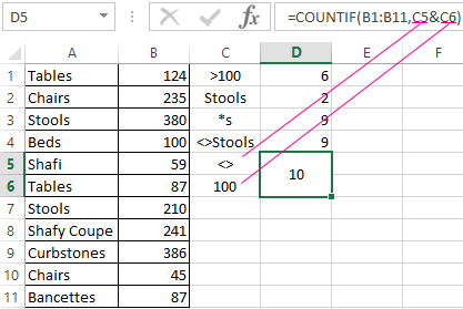
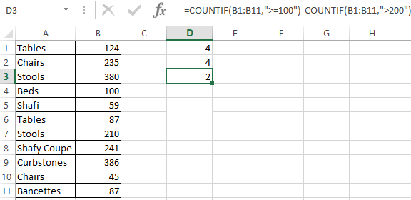
Formula: =COUNTIF(A1:A11,»<>»&»Stools»). The operator «<>» means «not equal». The ampersand sign (&) is used to merge this operator and the “Stools” value.

When you apply a reference, the formula will look like this:

Often you need to perform the COUNTIF function in Excel by two criteria. In this way, you can significantly expand its capabilities. Let’s consider special cases of using the COUNTIF function in Excel and examples with two criteria.

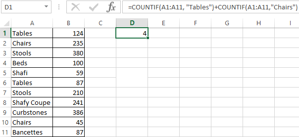
1. Let’s count how many cells are contained in the » Tables » and » Chairs » text. Formula:

   To specify several criteria, several COUNTIF phrases are used. They are united by the «+» operator.



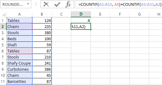
2. Criteria – cell references. Formula:

   The function searches for » Tables » text in cell A1 and » Chairs » text – in cell A2 based on the criterion.



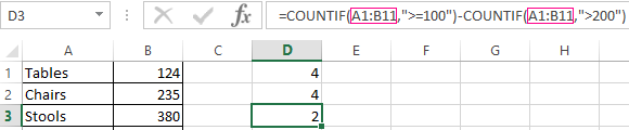
3. Count the number of cells in B1:B11 range with a value greater than or equal to 100 and less than or equal to 200. Formula:



4. Apply several ranges in the COUNTIF function. This is possible if the ranges are contiguous. It searches for values by two criteria in two columns simultaneously. If the ranges are not adjacent, then the COUNTIFS function is used.



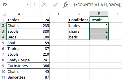
5. When the criterion is a reference to a range of cells with conditions, the function returns the array. To enter a formula, you need to highlight as many cells as the range with criteria contains. After entering the arguments, simultaneously press Shift + Ctrl + Enter control key combination. Excel recognizes the formula of the array.

COUNTIF with two criteria in Excel is very often used for automated and efficient data handling. Therefore, an advanced user is highly recommended to carefully study all of the examples above.

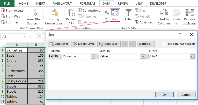
Subtotal command and the countif function

Count the number of goods sold in groups.

1. First, sort the table so that the same values are close.



2. The first argument of the formula “SUBTOTAL” – “Function number”. These are numbers from 1 to 11, indicating a statistical function for calculating the intermediate result. Counting the number of cells is carried out under number «2» (“COUNT”).

Download example COUNTIF in Excel

The formula has found the number of values for the «Chairs» group. For a large number of rows (more than a thousand), this combination of functions can be useful.

As the name suggests Excel COUNTIF Function is a combination of Count and IF formula. In plain English, COUNTIF Function can be described as a formula that can be used for counting the number of cells that fulfill a particular condition, within a predefined range.

How Excel Defines COUNTIF Function

Microsoft Excel defines COUNTIF as a formula that, “Counts the number of cells within a range that meet the given condition”.

This definition clearly explains that: COUNTIF Function is a better and sophisticated type of COUNT formula that gives you control over, which cells you wish to count.

Syntax of Excel COUNTIF Formula

Excel COUNTIF formula can be written as follows:

=COUNTIF(range , criteria)

Here ‘range’ specifies the range of cells over which you want to apply the ‘criteria‘.

‘criteria’ specifies the condition that a particular cell content should meet to be counted.

How to Use COUNTIF in Excel

Now, let’s see how to use the COUNTIF function in Excel.

Let’s consider, we have an Employee table as shown in the below image.

Objective: From the above table, our objective is to find the number of employees who have joined before 1990.

So, we will try to use the COUNTIF Formula to find the result.

range: In this case, ‘range’ will be “B2:B11”, as on these cells we have to apply the ‘criteria’.

criteria: In this case, ‘ criteria’ is “<01/01/1990”. This specifies that we want to count only those employees that are joined before 1^st January 1990.

This results in 6, which means there are 6 employees that have joined before 1990.

Few Important Facts About the COUNTIF Formula

1. COUNTIF formula only accepts a solid range, you cannot give multiple broken ranges to it. For example, COUNTIF cannot be written as

=COUNTIF(A1:A4 , A6:A8, ">0") //This is wrong
=COUNTIF(A1:A8, ">0") //This is correct


2. COUNTIF can accept wildcard characters (like “*” and “?”) in the ‘criteria’ argument. This means that you can write a COUNTIF as

=COUNTIF(D1:D15, "*o*")

This will count all the cells containing the “o” character, within the D1:D5 range.

3. As you know, the output of COUNTIF is an integer so you can also add two COUNTIF functions. For example: if you want to find the cells with value as “1” and cells with value as “2”, so you can use COUNTIF as

=COUNTIF(A1:A10,"1")+COUNTIF(A1:A10,"2")

4. COUNTIF throws a #NAME? error, if you supply an incorrect range to it.

Few Basic Examples of COUNTIF Function

In the above image, I have used an Employee table to depict how the COUNTIF function can be used.

Example 1: In the first example, I have used the Excel COUNTIF formula for finding the number of employees whose first name starts with “G”.

For this, I have used formula as

=COUNTIF(A3:A12,"G*")

Here, the COUNTIF Function scans the whole range from A3:A12 and tries to find a pattern “G*” (‘*’ is a wildcard operator which denotes any number of characters). The resultant is 2, as there are only two persons in the specified range whose first name starts with G.

Example 2: In the second example, I have used a COUNTIF function to find the cells which contain an Employee ID value greater than “26000”.

To accomplish this I have used a formula

=COUNTIF(C3:C12,">26000")

This formula searches the specified range for a value that specifies the criteria (i.e. >26000). So, the result is 5 as only 5 employees have an Employee ID greater than 26000.

Example 3: In the third example, I have fetched the number of employees whose salary is less than 4000.

To get this, I have again used a COUNTIF formula as

=COUNTIF(D3:D12,"<4000")

So, here the COUNTIF counts only those cells where salary range i.e. D3:D12 has a value less than 4000 and the resultant is 3.

Example 4: In the fourth example, I have used the following  formula

=COUNTIF(B3:B12,B5)

This formula finds the number of cells equal to the value of the cell B5 (i.e. “Massiot”), in the range B3:B15.

Here, first, the COUNTIF function finds the value at the B5 cell, and then it compares all the cells within the specified range with this value.

The resultant is 2 as only two records match the value at the B5 cell.

Example 5: In the above example, I had to find the total count of cells that contain “Apple” or “Peach”.

This can be easily done by adding the resultants of two COUNTIF statements like:

=COUNTIF(A2:A7,"Apple")+COUNTIF(A2:A7,"Peach")

The first COUNTIF statement gives the number of cells with a value equal to “Apple” and the second statement gives the count of cells with “Peach”. And hence the output comes out as 2+1=3.

Example 6: In this example (i.e. =COUNTIF(A,"Pear")), I have tried to show you what happens if you enter an incorrect range in the COUNTIF function.

In such cases, it throws a #NAME? error.

Few Advanced Examples of COUNTIF Function

Now, let’s see some practical examples of COUNTIF Function.

Example 7: Finding duplicate values using the COUNTIF function.

Let’s say we have a table as below, and we have to find the duplicate records in it.

For finding the duplicate records, we have used the formula:

=COUNTIF($A$2:$A$16,A2)>1

When this formula encounters a duplicate record it returns TRUE, while FALSE means that the record is Unique.

If you are wondering what these dollar ($) signs are doing in this formula, then you should read this post.

Recommended Reading: Find and Delete Duplicate cells in Excel

Example 8: Use the COUNTIF formula for generating the sorting order of a list.

Let’s consider we have a list as below.

Now, If we just want to know the alphabetic sorting order (in ascending order) of the employee names, then we can use the formula:

=COUNTIF($A$2:$A$15,"<="&A2)

See the below image, to see this formula in action.

As you can see, that this formula generates a number in-front of every employee. This number is the sorting order (in ascending sort) of the Employee Names.

Recommended Reading: How to alphabetize a list in Excel

So, this was all from my side. Do share your ideas and experiences related to Excel COUNTIF Function in the below comments section.

СЧЕТЕСЛИ в Excel — примеры функции с одним и несколькими условиями

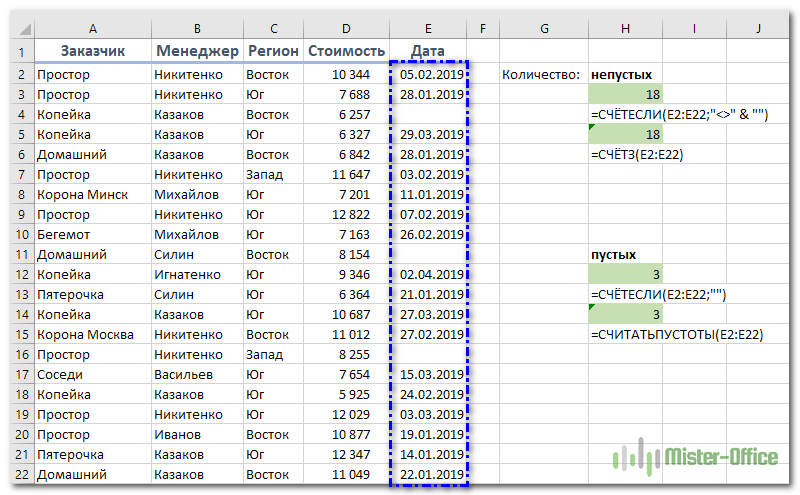
В этой статье мы сосредоточимся на функции Excel СЧЕТЕСЛИ (COUNTIF в английском варианте), которая предназначена для подсчета ячеек с определённым условием. Сначала мы кратко рассмотрим синтаксис и общее использование, а затем я приведу ряд примеров и предупрежу о возможных причудах при подсчете по нескольким критериям одновременно или же с определёнными типами данных.

По сути,они одинаковы во всех версиях, поэтому вы можете использовать примеры в MS Excel 2016, 2013, 2010 и 2007.

1. Примеры работы функции СЧЕТЕСЛИ.
   • Для подсчета текста.
   • Подсчет ячеек, начинающихся или заканчивающихся определенными символами
   • Подсчет чисел по условию.
   • Примеры с датами.
2. Как посчитать количество пустых и непустых ячеек?
3. Нулевые строки.
4. СЧЕТЕСЛИ с несколькими условиями.
   • Количество чисел в диапазоне
   • Количество ячеек с несколькими условиями ИЛИ.
5. Использование СЧЕТЕСЛИ для подсчета дубликатов.
   • 1. Ищем дубликаты в одном столбце
   • 2. Сколько совпадений между двумя столбцами?
   • 3. Сколько дубликатов и уникальных значений в строке?
6. Часто задаваемые вопросы и проблемы.

Функция Excel СЧЕТЕСЛИ применяется для подсчета количества ячеек в указанном диапазоне, которые соответствуют определенному условию.

Например, вы можете воспользоваться ею, чтобы узнать, сколько ячеек в вашей рабочей таблице содержит число, больше или меньше указанной вами величины. Другое стандартное использование — для подсчета ячеек с определенным словом или с определенной буквой (буквами).

СЧЕТЕСЛИ(диапазон; критерий)

Как видите, здесь только 2 аргумента, оба из которых являются обязательными:

• диапазон — определяет одну или несколько клеток для подсчета. Вы помещаете диапазон в формулу, как обычно, например, A1: A20.
• критерий — определяет условие, которое определяет, что именно считать. Это может быть число, текстовая строка, ссылка или выражение. Например, вы можете употребить  следующие критерии: «10», A2, «> = 10», «какой-то текст».

Что нужно обязательно запомнить?

• В аргументе «критерий» условие всегда нужно записывать в кавычках, кроме случая, когда используется ссылка либо какая-то функция.
• Любой из аргументов ссылается на диапазон из другой книги Excel, то эта книга должна быть открыта.
• Регистр букв не учитывается.
• Также можно применить знаки подстановки * и ? (о них далее – подробнее).
• Чтобы избежать ошибок, в тексте не должно быть непечатаемых знаков.

Как видите, синтаксис очень прост. Однако, он допускает множество возможных вариаций условий, в том числе символы подстановки, значения других ячеек и даже другие функции Excel. Это разнообразие делает функцию СЧЕТЕСЛИ действительно мощной и пригодной для многих задач, как вы увидите в следующих примерах.

Примеры работы функции СЧЕТЕСЛИ.

Для подсчета текста.

Давайте разбираться, как это работает. На рисунке ниже вы видите список заказов, выполненных менеджерами. Выражение  =СЧЕТЕСЛИ(В2:В22,»Никитенко») подсчитывает, сколько раз этот работник присутствует в списке:

Замечание. Критерий не чувствителен к регистру букв, поэтому можно вводить как прописные, так и строчные буквы.

Если ваши данные содержат несколько вариантов слов, которые вы хотите сосчитать, то вы можете использовать подстановочные знаки для подсчета всех ячеек, содержащих определенное слово, фразу или буквы, как часть их содержимого.

К примеру, в нашей таблице есть несколько заказчиков «Корона» из разных городов. Нам необходимо подсчитать общее количество заказов «Корона» независимо от города.

=СЧЁТЕСЛИ(A2:A22;»*Коро*»)

Мы подсчитали количество заказов, где в наименовании заказчика встречается «коро» в любом регистре. Звездочка (*) используется для поиска ячеек с любой последовательностью начальных и конечных символов, как показано в приведенном выше примере. Если вам нужно заменить какой-либо один символ, введите вместо него знак вопроса (?).

Кроме того, указывать условие прямо в формуле не совсем рационально, так как при необходимости подсчитать какие-то другие значения вам придется корректировать её. А это не слишком удобно.

Рекомендуется условие записывать в какую-либо ячейку и затем ссылаться на нее. Так мы сделали в H9. Также можно употребить подстановочные знаки со ссылками с помощью оператора конкатенации (&). Например, вместо того, чтобы указывать «* Коро *» непосредственно в формуле, вы можете записать его куда-нибудь, и использовать следующую конструкцию для подсчета ячеек, содержащих «Коро»:

=СЧЁТЕСЛИ(A2:A22;»*»&H8&»*»)

Подсчет ячеек, начинающихся или заканчивающихся определенными символами

Вы можете употребить подстановочный знак звездочку (*) или знак вопроса (?) в зависимости от того, какого именно результата вы хотите достичь.

Если вы хотите узнать количество ячеек, которые начинаются или заканчиваются определенным текстом, независимо от того, сколько имеется других символов, используйте:

=СЧЁТЕСЛИ(A2:A22;»К*») — считать значения, которые начинаются с « К» .

=СЧЁТЕСЛИ(A2:A22;»*р») — считать заканчивающиеся буквой «р».

Если вы ищете количество ячеек, которые начинаются или заканчиваются определенными буквами и содержат точное количество символов, то поставьте вопросительный знак (?):

=СЧЁТЕСЛИ(С2:С22;»????д») — находит количество буквой «д» в конце и текст в которых состоит из 5 букв, включая пробелы.

= СЧЁТЕСЛИ(С2:С22,»??») — считает количество состоящих из 2 символов, включая пробелы.

Примечание. Чтобы узнать количество клеток, содержащих в тексте знак вопроса или звездочку, введите тильду (~) перед символом ? или *.

Например, = СЧЁТЕСЛИ(С2:С22,»*~?*») будут подсчитаны все позиции, содержащие знак вопроса в диапазоне С2:С22.

Подсчет чисел по условию.

В отношении чисел редко случается, что нужно подсчитать количество их, равных какому-то определённому числу. Тем не менее, укажем, что записать нужно примерно следующее:

= СЧЁТЕСЛИ(D2:D22,10000)

Гораздо чаще нужно высчитать количество значений, больших либо меньших определенной величины.

Чтобы подсчитать значения, которые больше, меньше или равны указанному вами числу, вы просто добавляете соответствующий критерий, как показано в таблице ниже.

Обратите внимание, что математический оператор вместе с числом всегда заключен в кавычки .

критерии		Описание
Если больше, чем	=СЧЕТЕСЛИ(А2:А10;»>5″)	Подсчитайте, где значение больше 5.
Если меньше чем	=СЧЕТЕСЛИ(А2:А10;»>5″)	Подсчет со числами менее 5.
Если равно	=СЧЕТЕСЛИ(А2:А10;»=5″)	Определите, сколько раз значение равно 5.
Если не равно	=СЧЕТЕСЛИ(А2:А10;»<>5″)	Подсчитайте, сколько раз не равно 5.
Если больше или равно	=СЧЕТЕСЛИ(А2:А10;»>=5″)	Подсчет, когда больше или равно 5.
Если меньше или равно	=СЧЕТЕСЛИ(А2:А10;»<=5″)	Подсчет, где меньше или равно 5.

В нашем примере

=СЧЁТЕСЛИ(D2:D22;»>10000″)

Считаем количество крупных заказов на сумму более 10 000. Обратите внимание, что условие подсчета мы записываем здесь в виде текстовой строки и поэтому заключаем его в двойные кавычки.

Вы также можете использовать все вышеприведенные варианты для подсчета ячеек на основе значения другой ячейки. Вам просто нужно заменить число ссылкой.

Замечание. В случае использования ссылки, вы должны заключить математический оператор в кавычки и добавить амперсанд (&) перед ним. Например, чтобы подсчитать числа в диапазоне D2: D9, превышающие D3, используйте =СЧЕТЕСЛИ(D2:D9,»>»&D3)

Если вы хотите сосчитать записи, которые содержат математический оператор, как часть их содержимого, то есть символ «>», «<» или «=», то употребите в условиях подстановочный знак с оператором. Такие критерии будут рассматриваться как текстовая строка, а не числовое выражение.

Например, =СЧЕТЕСЛИ(D2:D9,»*>5*») будет подсчитывать все позиции в диапазоне D2: D9 с таким содержимым, как «Доставка >5 дней» или «>5 единиц в наличии».

Примеры с датами.

Если вы хотите сосчитать клетки с датами, которые больше, меньше или равны указанной вами дате, вы можете воспользоваться уже знакомым способом, используя формулы, аналогичные тем, которые мы обсуждали чуть выше. Все вышеприведенное работает как для дат, так и для чисел.

Позвольте привести несколько примеров:

критерии		Описание
Даты, равные указанной дате.	=СЧЕТЕСЛИ(E2:E22;»01.02.2019″)	Подсчитывает количество ячеек в диапазоне E2:E22 с датой 1 июня 2014 года.
Даты больше или равные другой дате.	=СЧЕТЕСЛИ(E2:E22,»>=01.02.2019″)	Сосчитайте количество ячеек в диапазоне E2:E22 с датой, большей или равной 01.06.2014.
Даты, которые больше или равны дате в другой ячейке, минус X дней.	=СЧЕТЕСЛИ(E2:E22,»>=»&H2-7)	Определите количество ячеек в диапазоне E2:E22 с датой, большей или равной дате в H2, минус 7 дней.

Помимо этих стандартных способов, вы можете употребить функцию СЧЕТЕСЛИ в сочетании с функциями даты и времени, например, СЕГОДНЯ(), для подсчета ячеек на основе текущей даты.

критерии
Равные текущей дате.	=СЧЕТЕСЛИ(E2:E22;СЕГОДНЯ())
До текущей даты, то есть меньше, чем сегодня.	=СЧЕТЕСЛИ(E2:E22;»<«&СЕГОДНЯ())
После текущей даты, т.е. больше, чем сегодня.	=СЧЕТЕСЛИ(E2:E22;»>»& ЕГОДНЯ ())
Даты, которые должны наступить через неделю.	= СЧЕТЕСЛИ(E2:E22,»=»&СЕГОДНЯ()+7)
В определенном диапазоне времени.	=СЧЁТЕСЛИ(E2:E22;»>=»&СЕГОДНЯ()+30)-СЧЁТЕСЛИ(E2:E22;»>»&СЕГОДНЯ())

Как посчитать количество пустых и непустых ячеек?

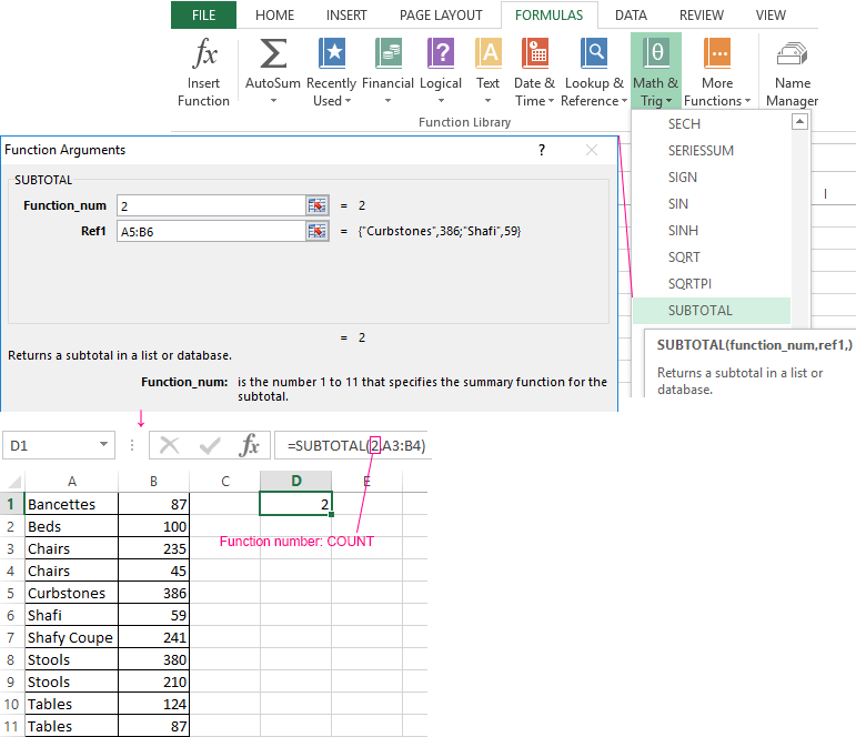
Посмотрим, как можно применить функцию СЧЕТЕСЛИ в Excel для подсчета количества пустых или непустых ячеек в указанном диапазоне.

Непустые.

В некоторых руководствах по работе с СЧЕТЕСЛИ вы можете встретить предложения для подсчета непустых ячеек, подобные этому:

СЧЕТЕСЛИ(диапазон;»*»)

Но дело в том, что приведенное выше выражение подсчитывает только клетки, содержащие любые текстовые значения. А это означает, что те из них, что включают даты и числа, будут обрабатываться как пустые (игнорироваться) и не войдут в общий итог!

Если вам нужно универсальное решение для подсчета всех непустых ячеек в указанном диапазоне, то введите:

СЧЕТЕСЛИ(диапазон;»<>» & «»)

Это корректно работает со всеми типами значений — текстом, датами и числами — как вы можете видеть на рисунке ниже.

Также непустые ячейки в диапазоне можно подсчитать:

=СЧЁТЗ(E2:E22).

Пустые.

Если вы хотите сосчитать пустые позиции в определенном диапазоне, вы должны придерживаться того же подхода — используйте в условиях символ подстановки для текстовых значений и параметр “” для подсчета всех пустых ячеек.

Считаем клетки, не содержащие текст:

СЧЕТЕСЛИ( диапазон; «<>» & «*»)

Поскольку звездочка (*) соответствует любой последовательности текстовых символов, в расчет принимаются клетки, не равные *, т.е. не содержащие текста в указанном диапазоне.

Для подсчета пустых клеток (все типы значений):

=СЧЁТЕСЛИ(E2:E22;»»)

Конечно, для таких случаев есть и специальная функция

=СЧИТАТЬПУСТОТЫ(E2:E22)

Но не все знают о ее существовании. Но вы теперь в курсе …

Нулевые строки.

Также имейте в виду, что СЧЕТЕСЛИ и СЧИТАТЬПУСТОТЫ считают ячейки с пустыми строками, которые только на первый взгляд выглядят пустыми.

Что такое эти пустые строки? Они также часто возникают при импорте данных из других программ (например, 1С). Внешне в них ничего нет, но на самом деле это не так. Если попробовать найти такие «пустышки» (F5 -Выделить — Пустые ячейки) — они не определяются. Но фильтр данных при этом их видит как пустые и фильтрует как пустые.

Дело в том, что существует такое понятие, как «строка нулевой длины» (или «нулевая строка»). Нулевая строка возникает, когда программе нужно вставить какое-то значение, а вставить нечего.

Проблемы начинаются тогда, когда вы пытаетесь с ней произвести какие-то математические вычисления (вычитание, деление, умножение и т.д.). Получите сообщение об ошибке #ЗНАЧ!. При этом функции СУММ и СЧЕТ их игнорируют, как будто там находится текст. А внешне там его нет.

И самое интересное — если указать на нее мышкой и нажать Delete (или вкладка Главная — Редактирование — Очистить содержимое) — то она становится действительно пустой, и с ней начинают работать формулы и другие функции Excel без всяких ошибок.

Если вы не хотите рассматривать их как пустые, используйте для подсчета реально пустых клеток следующее выражение:

=ЧСТРОК(E2:E22)*ЧИСЛСТОЛБ(E2:E22)-СЧЁТЕСЛИ(E2:E22;»<>»&»»)

Откуда могут появиться нулевые строки в ячейках? Здесь может быть несколько вариантов:

1. Он есть там изначально, потому что именно так настроена выгрузка и создание файлов в сторонней программе (вроде 1С). В некоторых случаях такие выгрузки настроены таким образом, что как таковых пустых ячеек нет — они просто заполняются строкой нулевой длины.
2. Была создана формула, результатом которой стал текст нулевой длины. Самый простой случай:

=ЕСЛИ(Е1=1;10;»»)

В итоге, если в Е1 записано что угодно, отличное от 1, программа вернет строку нулевой длины. И если впоследствии формулу заменять значением (Специальная вставка – Значения), то получим нашу псевдо-пустую позицию.

Если вы проверяете какие-то условия при помощи функции ЕСЛИ и в дальнейшем планируете производить с результатами математические действия, то лучше вместо «» ставьте 0. Тогда проблем не будет. Нули всегда можно заменить или скрыть: Файл -Параметры -Дополнительно — Показывать нули в позициях, которые содержат нулевые значения.

СЧЕТЕСЛИ с несколькими условиями.

На самом деле функция Эксель СЧЕТЕСЛИ не предназначена для расчета количества ячеек по нескольким условиям. В большинстве случаев я рекомендую использовать его множественный аналог — функцию СЧЕТЕСЛИМН. Она как раз и предназначена для вычисления количества ячеек, которые соответствуют двум или более условиям (логика И). Однако, некоторые задачи могут быть решены путем объединения двух или более функций СЧЕТЕСЛИ в одно выражение.

Количество чисел в диапазоне

Одним из наиболее распространенных применений функции СЧЕТЕСЛИ с двумя критериями является определение количества чисел в определенном интервале, т.е. меньше X, но больше Y.

Например, вы можете использовать для вычисления ячеек в диапазоне B2: B9, где значение больше 5 и меньше или равно 15:

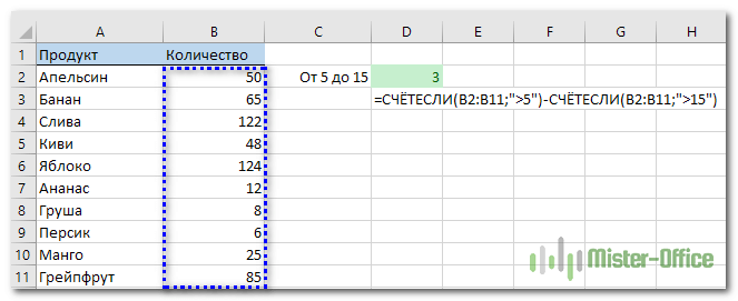
=СЧЁТЕСЛИ(B2:B11;»>5″)-СЧЁТЕСЛИ(B2:B11;»>15″)

Количество ячеек с несколькими условиями ИЛИ.

Когда вы хотите найти количество нескольких различных элементов в диапазоне, добавьте 2 или более функций СЧЕТЕСЛИ в выражение. Предположим, у вас есть список покупок, и вы хотите узнать, сколько в нем безалкогольных напитков.

Сделаем это:

=СЧЁТЕСЛИ(A4:A13;»Лимонад»)+СЧЁТЕСЛИ(A2:A11;»*сок»)

Обратите внимание, что мы включили подстановочный знак (*) во второй критерий. Он используется для вычисления количества всех видов сока в списке.

Как вы понимаете, сюда можно добавить и больше условий.

Использование СЧЕТЕСЛИ для подсчета дубликатов.

Другое возможное использование функции СЧЕТЕСЛИ в Excel — для поиска дубликатов в одном столбце, между двумя столбцами или в строке.

1. Ищем дубликаты в одном столбце

Эта простое выражение СЧЁТЕСЛИ($A$2:$A$24;A2)>1 найдет все одинаковые записи в A2: A24.

А другая формула СЧЁТЕСЛИ(B2:B24;ИСТИНА) сообщит вам, сколько существует дубликатов:

Для более наглядного представления найденных совпадений я использовал условное форматирование значения ИСТИНА.

2. Сколько совпадений между двумя столбцами?

Сравним список2 со списком1. В столбце Е берем последовательно каждое значение из списка2 и считаем, сколько раз оно встречается в списке1. Если совпадений ноль, значит это уникальное значение. На рисунке такие выделены цветом при помощи условного форматирования.

Выражение  =СЧЁТЕСЛИ($A$2:$A$24;C2) копируем вниз по столбцу Е.

Аналогичный расчет можно сделать и наоборот – брать значения из первого списка и искать дубликаты во втором.

Для того, чтобы просто определить количество дубликатов, можно использовать комбинацию функций СУММПРОИЗВ и СЧЕТЕСЛИ.

=СУММПРОИЗВ((СЧЁТЕСЛИ(A2:A24;C2:C24)>0)*(C2:C24<>»»))

Подсчитаем количество уникальных значений в списке2:

=СУММПРОИЗВ((СЧЁТЕСЛИ(A2:A24;C2:C24)=0)*(C2:C24<>»»))

Получаем 7 уникальных записей и 16 дубликатов, что и видно на рисунке.

Полезное. Если вы хотите выделить дублирующиеся позиции или целые строки, содержащие повторяющиеся записи, вы можете создать правила условного форматирования на основе формул СЧЕТЕСЛИ, как показано в этом руководстве — правила условного форматирования Excel.

3. Сколько дубликатов и уникальных значений в строке?

Если нужно сосчитать дубликаты или уникальные значения в определенной строке, а не в столбце, используйте одну из следующих формул. Они могут быть полезны, например, для анализа истории розыгрыша лотереи.

Считаем количество дубликатов:

=СУММПРОИЗВ((СЧЁТЕСЛИ(A2:K2;A2:K2)>1)*(A2:K2<>»»))

Видим, что 13 выпадало 2 раза.

Подсчитать уникальные значения:

=СУММПРОИЗВ((СЧЁТЕСЛИ(A2:K2;A2:K2)=1)*(A2:K2<>»»))

Часто задаваемые вопросы и проблемы.

Я надеюсь, что эти примеры помогли вам почувствовать функцию Excel СЧЕТЕСЛИ. Если вы попробовали какую-либо из приведенных выше формул в своих данных и не смогли заставить их работать или у вас возникла проблема, взгляните на следующие 5 наиболее распространенных проблем. Есть большая вероятность, что вы найдете там ответ или же полезный совет.

1. Возможен ли подсчет в несмежном диапазоне клеток?

Вопрос: Как я могу использовать СЧЕТЕСЛИ для несмежного диапазона или ячеек?

Ответ: Она не работает с несмежными диапазонами, синтаксис не позволяет указывать несколько отдельных ячеек в качестве первого параметра. Вместо этого вы можете использовать комбинацию нескольких функций СЧЕТЕСЛИ:

Неправильно: =СЧЕТЕСЛИ(A2;B3;C4;»>0″)

Правильно: = СЧЕТЕСЛИ (A2;»>0″) + СЧЕТЕСЛИ (B3;»>0″) + СЧЕТЕСЛИ (C4;»>0″)

Альтернативный способ — использовать функцию ДВССЫЛ (INDIRECT) для создания массива из несмежных клеток. Например, оба приведенных ниже варианта дают одинаковый результат, который вы видите на картинке:

=СУММ(СЧЁТЕСЛИ(ДВССЫЛ({«B2:B11″;»D2:D11″});»=0»))

Или же

=СЧЕТЕСЛИ($B2:$B11;0) + СЧЕТЕСЛИ($D2:$D11;0)

1. Амперсанд и кавычки в формулах СЧЕТЕСЛИ

Вопрос: когда мне нужно использовать амперсанд?

Ответ: Это, пожалуй, самая сложная часть функции СЧЕТЕСЛИ, что лично меня тоже смущает. Хотя, если вы подумаете об этом, вы увидите — амперсанд и кавычки необходимы для построения текстовой строки для аргумента.

Итак, вы можете придерживаться этих правил:

• Если вы используете число или ссылку на ячейку в критериях точного соответствия, вам не нужны ни амперсанд, ни кавычки. Например:

= СЧЕТЕСЛИ(A1:A10;10) или = СЧЕТЕСЛИ(A1:A10;C1)

• Если ваши условия содержат текст, подстановочный знак или логический оператор с числом, заключите его в кавычки. Например:

= СЧЕТЕСЛИ(A2:A10;»яблоко») или = СЧЕТЕСЛИ(A2:A10;»*») или = СЧЕТЕСЛИ(A2:A10;»>5″)

• Если ваши критерии — это выражение со ссылкой или же какая-то другая функция Excel, вы должны использовать кавычки («») для начала текстовой строки и амперсанд (&) для конкатенации (объединения) и завершения строки. Например:

= СЧЕТЕСЛИ(A2:A10;»>»&D2) или = СЧЕТЕСЛИ(A2:A10;»<=»&СЕГОДНЯ())

Если вы сомневаетесь, нужен ли амперсанд или нет, попробуйте оба способа. В большинстве случаев амперсанд работает просто отлично.

Например, = СЧЕТЕСЛИ(C2: C8;»<=5″) и = СЧЕТЕСЛИ(C2: C8;»<=»&5) работают одинаково хорошо.

1. Как сосчитать ячейки по цвету?

Вопрос: Как подсчитать клетки по цвету заливки или шрифта, а не по значениям?

Ответ: К сожалению, синтаксис функции не позволяет использовать форматы в качестве условия. Единственный возможный способ суммирования ячеек на основе их цвета — использование макроса или, точнее, пользовательской функции Excel VBA.

1. Ошибка #ИМЯ?

Проблема: все время получаю ошибку #ИМЯ? Как я могу это исправить?

Ответ: Скорее всего, вы указали неверный диапазон. Пожалуйста, проверьте пункт 1 выше.

1. Формула не работает

Проблема: моя формула не работает! Что я сделал не так?

Ответ: Если вы написали формулу, которая на первый взгляд верна, но она не работает или дает неправильный результат, начните с проверки наиболее очевидных вещей, таких как диапазон, условия, ссылки, использование амперсанда и кавычек.

Будьте очень осторожны с использованием пробелов. При создании одной из формул для этой статьи я был уже готов рвать волосы, потому что правильная конструкция (я точно знал, что это правильно!) не срабатывала. Как оказалось, проблема была на самом виду… Например, посмотрите на это: =СЧЁТЕСЛИ(A4:A13;» Лимонад»). На первый взгляд, нет ничего плохого, кроме дополнительного пробела после открывающей кавычки. Программа отлично проглотит всё без сообщения об ошибке, предупреждения или каких-либо других указаний. Но если вы действительно хотите посчитать товары, содержащие слово «Лимонад» и начальный пробел, то будете очень разочарованы….

Если вы используете функцию с несколькими критериями, разделите формулу на несколько частей и проверьте каждую из них отдельно.

И это все на сегодня. В следующей статье мы рассмотрим несколько способов подсчитывания ячеек в Excel с несколькими условиями.

Ещё примеры расчета суммы: