
Excel for Microsoft 365 Excel for Microsoft 365 for Mac Excel for the web Excel 2021 Excel 2021 for Mac Excel 2019 Excel 2019 for Mac Excel 2016 Excel 2016 for Mac Excel 2013 Excel Web App Excel 2010 Excel 2007 Excel for Mac 2011 Excel Starter 2010 More…Less
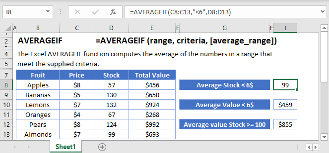
This article describes the formula syntax and usage of the AVERAGEIF
function in Microsoft Excel.
Description
Returns the average (arithmetic mean) of all the cells in a range that meet a given criteria.
Syntax
AVERAGEIF(range, criteria, [average_range])
The AVERAGEIF function syntax has the following arguments:
-
Range Required. One or more cells to average, including numbers or names, arrays, or references that contain numbers.
-
Criteria Required. The criteria in the form of a number, expression, cell reference, or text that defines which cells are averaged. For example, criteria can be expressed as 32, «32», «>32», «apples», or B4.
-
Average_range Optional. The actual set of cells to average. If omitted, range is used.
Remarks
-
Cells in range that contain TRUE or FALSE are ignored.
-
If a cell in average_range is an empty cell, AVERAGEIF ignores it.
-
If range is a blank or text value, AVERAGEIF returns the #DIV0! error value.
-
If a cell in criteria is empty, AVERAGEIF treats it as a 0 value.
-
If no cells in the range meet the criteria, AVERAGEIF returns the #DIV/0! error value.
-
You can use the wildcard characters, question mark (?) and asterisk (*), in criteria. A question mark matches any single character; an asterisk matches any sequence of characters. If you want to find an actual question mark or asterisk, type a tilde (~) before the character.
-
Average_range does not have to be the same size and shape as range. The actual cells that are averaged are determined by using the top, left cell in average_range as the beginning cell, and then including cells that correspond in size and shape to range. For example:
|
If range is |
And average_range is |
Then the actual cells evaluated are |
|---|---|---|
|
A1:A5 |
B1:B5 |
B1:B5 |
|
A1:A5 |
B1:B3 |
B1:B5 |
|
A1:B4 |
C1:D4 |
C1:D4 |
|
A1:B4 |
C1:C2 |
C1:D4 |
Note: The AVERAGEIF function measures central tendency, which is the location of the center of a group of numbers in a statistical distribution. The three most common measures of central tendency are:
-
Average which is the arithmetic mean, and is calculated by adding a group of numbers and then dividing by the count of those numbers. For example, the average of 2, 3, 3, 5, 7, and 10 is 30 divided by 6, which is 5.
-
Median which is the middle number of a group of numbers; that is, half the numbers have values that are greater than the median, and half the numbers have values that are less than the median. For example, the median of 2, 3, 3, 5, 7, and 10 is 4.
-
Mode which is the most frequently occurring number in a group of numbers. For example, the mode of 2, 3, 3, 5, 7, and 10 is 3.
For a symmetrical distribution of a group of numbers, these three measures of central tendency are all the same. For a skewed distribution of a group of numbers, they can be different.
Examples
Copy the example data in the following table, and paste it in cell A1 of a new Excel worksheet. For formulas to show results, select them, press F2, and then press Enter. If you need to, you can adjust the column widths to see all the data.
|
Property Value |
Commission |
|
|---|---|---|
|
100000 |
7000 |
|
|
200000 |
14000 |
|
|
300000 |
21000 |
|
|
400000 |
28000 |
|
|
Formula |
Description |
Result |
|
=AVERAGEIF(B2:B5,»<23000″) |
Average of all commissions less than 23000. Three of the four commissions meet this condition, and their total is 42000. |
14000 |
|
=AVERAGEIF(A2:A5,»<250000″) |
Average of all property values less than 250000. Two of the four property values meet this condition, and their total is 300000. |
150000 |
|
=AVERAGEIF(A2:A5,»<95000″) |
Average of all property values less than 95000. Because there are 0 property values that meet this condition, the AVERAGEIF function returns the #DIV/0! error because it tries to divide by 0. |
#DIV/0! |
|
=AVERAGEIF(A2:A5,»>250000″,B2:B5) |
Average of all commissions with a property value greater than 250000. Two commissions meet this condition, and their total is 49000. |
24500 |
Example 2
|
Region |
Profits (Thousands) |
|
|---|---|---|
|
East |
45678 |
|
|
West |
23789 |
|
|
North |
-4789 |
|
|
South (New Office) |
0 |
|
|
MidWest |
9678 |
|
|
Formula |
Description |
Result |
|
=AVERAGEIF(A2:A6,»=*West»,B2:B6) |
Average of all profits for the West and MidWest regions. |
16733.5 |
|
=AVERAGEIF(A2:A6,»<>*(New Office)»,B2:B6) |
Average of all profits for all regions excluding new offices. |
18589 |
Need more help?
Want more options?
Explore subscription benefits, browse training courses, learn how to secure your device, and more.
Communities help you ask and answer questions, give feedback, and hear from experts with rich knowledge.
Содержание
- AVERAGEIF function
- Want more?
- Функция AVERAGEIF (СРЗНАЧЕСЛИ) в Excel. Как использовать?
- Что возвращает функция
- Синтаксис
- Аргументы функции
- Дополнительная информация
- Примеры использования функции СРЗНАЧЕСЛИ в Excel
- Пример 1. Вычисляем среднее арифметическое по критерию
- Пример 2. Используем подстановочные знаки в функции СРЗНАЧЕСЛИ
- Пример 3. Используем операторы сравнения в функции СРЗНАЧЕСЛИ
- AVERAGEIF function
- Description
- Syntax
- Remarks
- Examples
- AVERAGEIFS function
- Description
- Syntax
- Remarks
- Examples
- AVERAGEIF & AVERAGEIFS Functions – Average Values If – Excel & Google Sheets
- AVERAGEIF Function Overview
- AVERAGEIF Function Syntax and Arguments:
- What is the AVERAGEIF function?
- Basic example
- Two-column example
- Working with Dates, Multiple criteria
- Multiple columns
- AVERAGEIFS with OR type logic
- Dealing with blanks
- AVERAGEIF in Google Sheets
AVERAGEIF function

The AVERAGEIF function returns the average of cells in a range that meet criteria you provide.
Want more?
The AVERAGEIF function returns the average of cells in a range that meet criteria you provide.
Let’s determine the average for sales that are greater than $60000.
Type an = sign, AVERAGEIF, opening parenthesis (in this example, we are going to evaluate and average the same range of cells, C2 through C5, in the Sales column), comma, then we type the criteria against which the range is evaluated, enclosed in quotes (you put it in quotes so Excel interprets the operator and value correctly), in this example, greater than 60000.
Don’t type a comma in 60000. Excel would interpret that as a separator for arguments of the function and return an error.
And press Enter. Excel automatically adds the closing parenthesis to the formula.
The average for sales greater than $60000 is $71229.
Let’s walk through this.
The function evaluates how many cells in the Sales column meet the criteria of greater than 60000. There are three cells.
The function then averages these cells.
Now we’ll use the AVERAGEIF function to determine the average for sales where the number of orders is greater than 50.
In this example, one range of cells is evaluated against the criteria and a second range of cells is averaged.
We type = AVERAGEIF, opening parenthesis, the range of cells we want evaluated (cells B2 through B5) in the number of orders column, comma, the criteria by which the range is to be evaluated enclosed in quotes (greater than 50), comma, the range of cells we want to average (cells C2 through C5 in the Sales column), and press Enter.
The average for sales where the number of orders is greater than 50 is $66487.
Let’s walk through this one, too.
First, the function evaluates which cells in B2 through B5 meet the criteria of greater than 50.
Three cells meet the criteria. The function then averages the cells from the Sales column where the criteria is met by the corresponding cell in column B.
For more information about the AVERAGEIF function, see the course summary at the end of the course.
Источник
Функция AVERAGEIF (СРЗНАЧЕСЛИ) в Excel. Как использовать?
Функция СРЗНАЧЕСЛИ (AVERAGEIF) в Excel используется для вычисления среднего арифметического по заданном диапазону данных и критерию.
Что возвращает функция
Возвращает число, обозначающее среднее арифметическое по заданному диапазону данных и критерию, указанному в качестве аргумента.
Синтаксис
=AVERAGEIF(range, criteria, [average_range]) — английская версия
=СРЗНАЧЕСЛИ(диапазон, условия, [диапазон_усреднения]) — русская версия
Аргументы функции
- range (диапазон) — диапазон ячеек, по которому будет осуществлена проверка на соответствие заданному критерию;
- criteria (условия) — критерий, по которому определяется какие значения из диапазона ячеек подходят для вычисления среднего арифметического;
- [average_range] ([диапазон_усреднения]) (Опционально) — диапазон ячеек, по которым функция осуществит вычисление среднего арифметического, при соответствии заданному критерию. Если этот аргумент не указан в формуле, функция производит вычисления по аргументу range(диапазон).
Дополнительная информация
- Пустые ячейки игнорируются при вычислении;
- Если в качестве критерия указана пустая ячейка, то функция воспринимает ее значение как «0»;
- Если ни одна ячейка из заданного диапазона не соответствует критерию, функция выдаст ошибку;
- Если диапазон ячеек пуст или содержит данные в текстовом формате, формула выдаст ошибку;
- Критерием может выступать число, выражение, ссылка на ячейку, текст или формула;
- Критерий, указанный в формате текста или логического/математического символа (=,+,-,/,*) следует указывать в двойных кавычках;
- Подстановочные знаки могут использоваться в качестве критерия.
Примеры использования функции СРЗНАЧЕСЛИ в Excel
Пример 1. Вычисляем среднее арифметическое по критерию
![]()
На примере выше функция проверяет список значений в диапазоне «А2:А6» на соответствие критерию «Андрей» и вычисляет по соответствующим критерию ячейкам среднее арифметическое в диапазоне ячеек «В2:В6».
Так как в диапазоне «А2:А6» указаны данные для двух ячеек «Андрей» — «62» и «19», то функция вычисляет среднее арифметическое — «40.5».
Пример 2. Используем подстановочные знаки в функции СРЗНАЧЕСЛИ
Вы можете использовать подстановочные знаки в критерии функции.
В Excel существует три подстановочных знака — ?, *,
- знак «?» — сопоставляет любой одиночный символ;
- знак «*» — сопоставляет любые дополнительные символы;
- знак «
» — используется, если нужно найти сам вопросительный знак или звездочку.
![]()
На примере выше, функция проверяет список данных в диапазоне «А2:А6» на соответствие критерию с подстановочными знаками «*а*», который подразумевает любые данные содержащие букву «а». Так как в диапазоне данных «А2:А6» этому критерию соответствуют все имена кроме «Олег» => среднее арифметическое будет вычислено по диапазону ячеек B2:B6 (исключая ячейку B5) = «29.5».
Пример 3. Используем операторы сравнения в функции СРЗНАЧЕСЛИ
![]()
В случаях, когда вы не указываете аргумент average_range (диапазон_усреднения), она, автоматически, производит расчеты из заданного диапазона ячеек в аргументе range (диапазон).
На примере выше, функция определяет по заданному критерию «>19» какие ячейки из диапазона «B2:B6» больше числа «19» и вычисляет по ним среднее арифметическое. Важно, любые операторы следует указывать в двойных кавычках!
Источник
AVERAGEIF function
This article describes the formula syntax and usage of the AVERAGEIF function in Microsoft Excel.
Description
Returns the average (arithmetic mean) of all the cells in a range that meet a given criteria.
Syntax
AVERAGEIF(range, criteria, [average_range])
The AVERAGEIF function syntax has the following arguments:
Range Required. One or more cells to average, including numbers or names, arrays, or references that contain numbers.
Criteria Required. The criteria in the form of a number, expression, cell reference, or text that defines which cells are averaged. For example, criteria can be expressed as 32, «32», «>32», «apples», or B4.
Average_range Optional. The actual set of cells to average. If omitted, range is used.
Cells in range that contain TRUE or FALSE are ignored.
If a cell in average_range is an empty cell, AVERAGEIF ignores it.
If range is a blank or text value, AVERAGEIF returns the #DIV0! error value.
If a cell in criteria is empty, AVERAGEIF treats it as a 0 value.
If no cells in the range meet the criteria, AVERAGEIF returns the #DIV/0! error value.
You can use the wildcard characters, question mark (?) and asterisk (*), in criteria. A question mark matches any single character; an asterisk matches any sequence of characters. If you want to find an actual question mark or asterisk, type a tilde (
) before the character.
Average_range does not have to be the same size and shape as range. The actual cells that are averaged are determined by using the top, left cell in average_range as the beginning cell, and then including cells that correspond in size and shape to range. For example:
And average_range is
Then the actual cells evaluated are
Note: The AVERAGEIF function measures central tendency, which is the location of the center of a group of numbers in a statistical distribution. The three most common measures of central tendency are:
Average which is the arithmetic mean, and is calculated by adding a group of numbers and then dividing by the count of those numbers. For example, the average of 2, 3, 3, 5, 7, and 10 is 30 divided by 6, which is 5.
Median which is the middle number of a group of numbers; that is, half the numbers have values that are greater than the median, and half the numbers have values that are less than the median. For example, the median of 2, 3, 3, 5, 7, and 10 is 4.
Mode which is the most frequently occurring number in a group of numbers. For example, the mode of 2, 3, 3, 5, 7, and 10 is 3.
For a symmetrical distribution of a group of numbers, these three measures of central tendency are all the same. For a skewed distribution of a group of numbers, they can be different.
Examples
Copy the example data in the following table, and paste it in cell A1 of a new Excel worksheet. For formulas to show results, select them, press F2, and then press Enter. If you need to, you can adjust the column widths to see all the data.
Источник
AVERAGEIFS function
This article describes the formula syntax and usage of the AVERAGEIFS function in Microsoft Excel.
Description
Returns the average (arithmetic mean) of all cells that meet multiple criteria.
Syntax
AVERAGEIFS(average_range, criteria_range1, criteria1, [criteria_range2, criteria2], . )
The AVERAGEIFS function syntax has the following arguments:
Average_range Required. One or more cells to average, including numbers or names, arrays, or references that contain numbers.
Criteria_range1, criteria_range2, … Criteria_range1 is required, subsequent criteria_ranges are optional. 1 to 127 ranges in which to evaluate the associated criteria.
Criteria1, criteria2, . Criteria1 is required, subsequent criteria are optional. 1 to 127 criteria in the form of a number, expression, cell reference, or text that define which cells will be averaged. For example, criteria can be expressed as 32, «32», «>32», «apples», or B4.
If average_range is a blank or text value, AVERAGEIFS returns the #DIV0! error value.
If a cell in a criteria range is empty, AVERAGEIFS treats it as a 0 value.
Cells in range that contain TRUE evaluate as 1; cells in range that contain FALSE evaluate as 0 (zero).
Each cell in average_range is used in the average calculation only if all of the corresponding criteria specified are true for that cell.
Unlike the range and criteria arguments in the AVERAGEIF function, in AVERAGEIFS each criteria_range must be the same size and shape as sum_range.
If cells in average_range cannot be translated into numbers, AVERAGEIFS returns the #DIV0! error value.
If there are no cells that meet all the criteria, AVERAGEIFS returns the #DIV/0! error value.
You can use the wildcard characters, question mark (?) and asterisk (*), in criteria. A question mark matches any single character; an asterisk matches any sequence of characters. If you want to find an actual question mark or asterisk, type a tilde (
) before the character.
Note: The AVERAGEIFS function measures central tendency, which is the location of the center of a group of numbers in a statistical distribution. The three most common measures of central tendency are:
Average which is the arithmetic mean, and is calculated by adding a group of numbers and then dividing by the count of those numbers. For example, the average of 2, 3, 3, 5, 7, and 10 is 30 divided by 6, which is 5.
Median which is the middle number of a group of numbers; that is, half the numbers have values that are greater than the median, and half the numbers have values that are less than the median. For example, the median of 2, 3, 3, 5, 7, and 10 is 4.
Mode which is the most frequently occurring number in a group of numbers. For example, the mode of 2, 3, 3, 5, 7, and 10 is 3.
For a symmetrical distribution of a group of numbers, these three measures of central tendency are all the same. For a skewed distribution of a group of numbers, they can be different.
Examples
Copy the example data in the following table, and paste it in cell A1 of a new Excel worksheet. For formulas to show results, select them, press F2, and then press Enter. If you need to, you can adjust the column widths to see all the data.
Источник
AVERAGEIF & AVERAGEIFS Functions – Average Values If – Excel & Google Sheets
This Tutorial demonstrates how to use the Excel AVERAGEIF and AVERAGEIFS Functions in Excel and Google Sheets to average data that meet certain criteria.
AVERAGEIF Function Overview
You can use the AVERAGEIF function in Excel to count cells that contain a specific value, count cells that are greater than or equal to a value, etc.
To use the AVERAGEIF Excel Worksheet Function, select a cell and type:
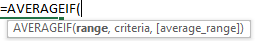
(Notice how the formula inputs appear)
AVERAGEIF Function Syntax and Arguments:
range – The range of cells to count.
criteria – The criteria that controls which cells should be counted.
average_range – [optional] The cells to average. When omitted, range is used.
What is the AVERAGEIF function?
The AVERAGEIF function is one of the older functions used in spreadsheets. It is used to scan through a range of cells checking for a specific criterion, and then giving the average (aka the mathematical mean) if the values in a range that correspond to those values. The original AVERAGEIF function was limited to just one criterion. After 2007, the AVERAGEIFS function was created which allows a multitude of criteria. Most of the general use remains the same between the two, but there are some critical differences in the syntax that we’ll discuss throughout this article.
If you haven’t already, you can review much of the similar structure and examples in the COUNTIFS article .
Basic example
Let’s consider this list of recorded sales, and we want to know the average income.
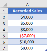
Because we had an expense, the negative value, we can’t just do a basic average. Instead, we want to average only the values that are greater than 0. The “greater than 0” is what will be our criteria in an AVERAGEIF function. Our formula to state this is
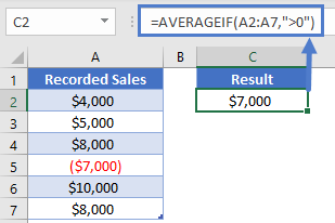
Two-column example
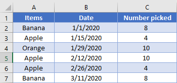
While the original AVERAGEIF function was designed to let you apply a criterion to the range of numbers you want to sum, much of the time you’ll need to apply one or more criteria to other columns. Let’s consider this table:
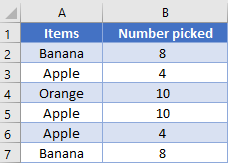
Now, if we use the original AVERAGEIF function to find out how many Bananas we have on average. We’ll put our criteria in cell D1, and we’ll need to give the range we want to average as the last argument, and so our formula would be
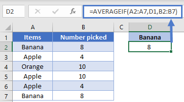
However, when programmers eventually realized that users wanted to give more than one criterion, the AVERAGEIFS function was created. In order to create one structure that would work for any number of criteria, the AVERAGEIFS requires that the sum range is listed first. In our example, this means that the formula needs to be
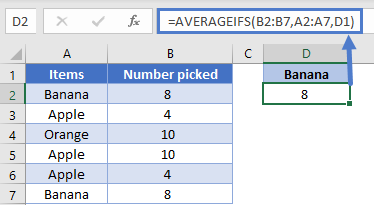
NOTE: These two formulas get the same result and can look similar, so pay close attention to which function is being used to make sure you list out all the arguments in the correct order.
Working with Dates, Multiple criteria
When working with dates in a spreadsheet, while it is possible to input the date directly into the formula, it’s best practice to have the date in a cell so that you can just reference the cell in a formula. For example, this helps the computer know that you’re wanting to use the date 5/27/2020, and not the number 5 divided by 27 divided by 2020.
Let’s look at our next table recording the number of visitors to a site every two weeks.
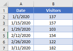
We can specify the start and end points of the range we want to look at in D2 and E2. Our formula then to find the average the number of visitors in this range could be:
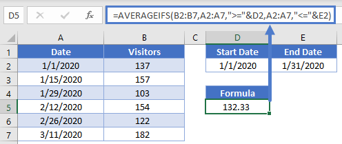
Note how we were able to concatenate the comparisons of “ =” to the cell references to create the criteria. Also, even though both criteria were being applied to the same range of cells (A2:A7), you need to write out the range twice, once per each criterion.
Multiple columns
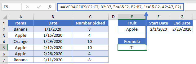
When using multiple criteria, you can apply them to the same range as we did with previous example, or you can apply them to different ranges. Let’s combine our sample data into this table:
We’ve setup some cells for the user to enter what they want to search for in cells E2 through G2. We thus need a formula that will add up the total number of apples picked in February. Our formula looks like this:
AVERAGEIFS with OR type logic
Up to this point, the examples we’ve used have all been AND based comparison, where we are looking for rows that meet all our criteria. Now, we’ll consider the case when you want to search for the possibility of a row meeting one or another criterion.
Let’s look at this list of sales:
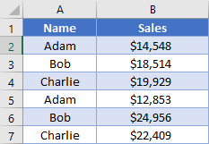
We’d like to add up the average sales for both Adam and Bob. First, a quick discussion about taking averages. If you have an uneven number of things such has 3 entries for Adam and 2 for Bob, you can’t simply take the average of each person’s sales. This is known as taking the average of averages, and you end up giving an unfair weighting to the item that has few entries. If this is the case with your data, you’d need to calculate an average the “manual” way: take the sum of all your items divided by the count of your items. To review how to do this, you can check out the articles here:
Now, if the number of entries is the same, such as in our table, then you have a couple options you can do. The simplest is to add two AVERAGEIFS together, like so, and then divide by 2 (the number of items in our list)
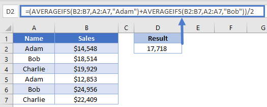
Here, we’ve had the computer calculate our individual scores, and then we add them together.
Our next option is good for when you have more criteria ranges, such that you don’t want to have to rewrite the whole formula repeatedly. In the previous formula, we manually told the computer to add two different AVERAGEIFS together. However, you can also do this by writing your criteria inside an array, like this:
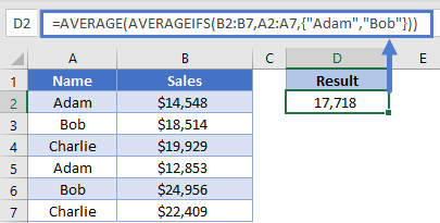
Look at how the array is constructed inside the curly brackets. When the computer evaluates this formula, it will know that we want to calculate an AVERAGEIFS function for each item in our array, thus creating an array of numbers. The outer AVERAGE function will then take that array of numbers and turn it into a single number. Stepping through the formula evaluation, it would look like this:
We get the same result, but we were able to write out the formula a bit more succinctly.
Dealing with blanks
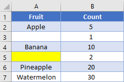
Sometimes your data set will have blank cells that you need to either find or avoid. Setting up the criteria for these can be a little tricky, so let’s look at another example.
![]()
Note that cell A3 is truly blank, while cell A5 has a formula returning a zero-length string of “”. If we want to find the total average of truly blank cells, we’d use a criterion of “=”, and our formula would look like this:
![]()
On the other hand, if we want to get the average for all cells that visually looks blank, we’ll change the criteria to be “”, and the formula looks like
![]()
Let’s flip it around: what if you want to find the average of non-blank cells? Unfortunately, the current design won’t let you avoid the zero-length string. You can use a criterion of “<>”, but as you can see in the example, it still includes the value from row 5.
![]()
If you need to not count cells containing zero length strings, you’ll want to consider using the LEN function inside a SUMPRODUCT
AVERAGEIF in Google Sheets
The AVERAGEIF Function works exactly the same in Google Sheets as in Excel:
Источник
Функция СРЗНАЧЕСЛИ (AVERAGEIF) в Excel используется для вычисления среднего арифметического по заданном диапазону данных и критерию.
Содержание
- Что возвращает функция
- Синтаксис
- Аргументы функции
- Дополнительная информация
- Примеры использования функции СРЗНАЧЕСЛИ в Excel
- Пример 1. Вычисляем среднее арифметическое по критерию
- Пример 2. Используем подстановочные знаки в функции СРЗНАЧЕСЛИ
- Пример 3. Используем операторы сравнения в функции СРЗНАЧЕСЛИ
Что возвращает функция
Возвращает число, обозначающее среднее арифметическое по заданному диапазону данных и критерию, указанному в качестве аргумента.
Синтаксис
=AVERAGEIF(range, criteria, [average_range]) — английская версия
=СРЗНАЧЕСЛИ(диапазон, условия, [диапазон_усреднения]) — русская версия
Аргументы функции
- range (диапазон) — диапазон ячеек, по которому будет осуществлена проверка на соответствие заданному критерию;
- criteria (условия) — критерий, по которому определяется какие значения из диапазона ячеек подходят для вычисления среднего арифметического;
- [average_range] ([диапазон_усреднения]) (Опционально) — диапазон ячеек, по которым функция осуществит вычисление среднего арифметического, при соответствии заданному критерию. Если этот аргумент не указан в формуле, функция производит вычисления по аргументу range(диапазон).
Дополнительная информация
- Пустые ячейки игнорируются при вычислении;
- Если в качестве критерия указана пустая ячейка, то функция воспринимает ее значение как «0»;
- Если ни одна ячейка из заданного диапазона не соответствует критерию, функция выдаст ошибку;
- Если диапазон ячеек пуст или содержит данные в текстовом формате, формула выдаст ошибку;
- Критерием может выступать число, выражение, ссылка на ячейку, текст или формула;
- Критерий, указанный в формате текста или логического/математического символа (=,+,-,/,*) следует указывать в двойных кавычках;
- Подстановочные знаки могут использоваться в качестве критерия.
Примеры использования функции СРЗНАЧЕСЛИ в Excel
Пример 1. Вычисляем среднее арифметическое по критерию

На примере выше функция проверяет список значений в диапазоне «А2:А6» на соответствие критерию «Андрей» и вычисляет по соответствующим критерию ячейкам среднее арифметическое в диапазоне ячеек «В2:В6».
Так как в диапазоне «А2:А6» указаны данные для двух ячеек «Андрей» — «62» и «19», то функция вычисляет среднее арифметическое — «40.5».
Больше лайфхаков в нашем Telegram Подписаться
Пример 2. Используем подстановочные знаки в функции СРЗНАЧЕСЛИ
Вы можете использовать подстановочные знаки в критерии функции.
В Excel существует три подстановочных знака — ?, *, ~.
- знак «?» — сопоставляет любой одиночный символ;
- знак «*» — сопоставляет любые дополнительные символы;
- знак «~» — используется, если нужно найти сам вопросительный знак или звездочку.
На примере выше, функция проверяет список данных в диапазоне «А2:А6» на соответствие критерию с подстановочными знаками «*а*», который подразумевает любые данные содержащие букву «а». Так как в диапазоне данных «А2:А6» этому критерию соответствуют все имена кроме «Олег» => среднее арифметическое будет вычислено по диапазону ячеек B2:B6 (исключая ячейку B5) = «29.5».
Пример 3. Используем операторы сравнения в функции СРЗНАЧЕСЛИ
В случаях, когда вы не указываете аргумент average_range (диапазон_усреднения), она, автоматически, производит расчеты из заданного диапазона ячеек в аргументе range (диапазон).
На примере выше, функция определяет по заданному критерию «>19» какие ячейки из диапазона «B2:B6» больше числа «19» и вычисляет по ним среднее арифметическое. Важно, любые операторы следует указывать в двойных кавычках!
Содержание
- Обзор функции СРЗНАЧЕСЛИ
- Синтаксис и аргументы функции СРЗНАЧЕСЛИ:
- Что такое функция СРЗНАЧЕСЛИ?
- AVERAGEIF в Google Таблицах
В этом руководстве показано, как использовать функции Excel AVERAGEIF и AVERAGEIFS в Excel и Google Sheets для усреднения данных, соответствующих определенным критериям.

Обзор функции СРЗНАЧЕСЛИ
Вы можете использовать функцию СРЗНАЧЕСЛИ в Excel для подсчета ячеек, содержащих определенное значение, подсчета ячеек, которые больше или равны значению и т. Д.
Чтобы использовать функцию рабочего листа Excel СРЗНАЧЕСЛИ, выберите ячейку и введите:

(Обратите внимание, как появляются входные данные формулы)
Синтаксис и аргументы функции СРЗНАЧЕСЛИ:
= СРЗНАЧЕСЛИ (диапазон; критерии; [средний_ диапазон])
диапазон — Диапазон подсчитываемых ячеек.
критерии — Критерии, определяющие, какие ячейки следует подсчитывать.
средний_ диапазон — [необязательно] Ячейки для усреднения. Если не указано, используется диапазон.
Что такое функция СРЗНАЧЕСЛИ?
Функция СРЗНАЧЕСЛИ — одна из старых функций, используемых в электронных таблицах. Он используется для сканирования диапазона ячеек, проверяя определенный критерий, а затем выдает среднее значение (также называемое математическим средним) для значений в диапазоне, которые соответствуют этим значениям. Исходная функция СРЗНАЧЕСЛИ ограничивалась только одним критерием. После 2007 года была создана функция СРЗНАЧЕСЛИМН, которая позволяет использовать множество критериев. В основном они используются одинаково, но есть некоторые важные различия в синтаксисе, которые мы обсудим в этой статье.
Если вы еще этого не сделали, вы можете просмотреть большую часть аналогичной структуры и примеры в статье СЧЁТЕСЛИМН.
Базовый пример
Давайте рассмотрим этот список зарегистрированных продаж, и мы хотим знать средний доход.

Поскольку у нас были расходы, отрицательное значение, мы не можем просто вычислить базовое среднее значение. Вместо этого мы хотим усреднить только те значения, которые больше 0. «Больше 0» — это то, что будет нашим критерием в функции СРЗНАЧЕСЛИ. Наша формула для утверждения, что это
= СРЗНАЧЕСЛИ (A2: A7; "> 0")

Пример с двумя столбцами
Хотя исходная функция СРЗНАЧЕСЛИ была разработана, чтобы позволить вам применить критерий к диапазону чисел, которые вы хотите суммировать, большую часть времени вам потребуется применить один или несколько критериев к другим столбцам. Рассмотрим эту таблицу:

Теперь, если мы воспользуемся исходной функцией СРЗНАЧЕСЛИ, чтобы узнать, сколько бананов у нас в среднем. Мы поместим наши критерии в ячейку D1, и нам нужно будет указать диапазон, который мы хотим в среднем в качестве последнего аргумента, и поэтому наша формула будет
= СРЗНАЧЕСЛИ (A2: A7; D1; B2: B7)

Однако, когда программисты в конце концов поняли, что пользователи хотят давать более одного критерия, была создана функция СРЗНАЧЕСЛИМН. Чтобы создать одну структуру, которая будет работать для любого количества критериев, для СРЕДНЕЛИН необходимо, чтобы диапазон сумм был указан первым. В нашем примере это означает, что формула должна быть
= СРЕДНЕЛИН (B2: B7; A2: A7; D1)

ПРИМЕЧАНИЕ. Эти две формулы дают одинаковый результат и могут выглядеть примерно одинаково, поэтому обратите особое внимание на то, какая функция используется, чтобы убедиться, что вы перечислили все аргументы в правильном порядке.
Работа с датами, несколько критериев
При работе с датами в электронной таблице, хотя можно ввести дату непосредственно в формулу, лучше всего иметь дату в ячейке, чтобы вы могли просто ссылаться на ячейку в формуле. Например, это помогает компьютеру понять, что вы хотите использовать дату 27.05.2020, а не число 5, разделенное на 27, разделенное на 2022 год.
Давайте посмотрим на нашу следующую таблицу, в которой регистрируется количество посетителей сайта каждые две недели.

Мы можем указать начальную и конечную точки диапазона, который мы хотим посмотреть в D2 и E2. Наша формула для определения среднего числа посетителей в этом диапазоне может быть:
= AVERAGEIFS (B2: B7, A2: A7, "> =" & D2, A2: A7, "<=" & E2)

Обратите внимание, как мы смогли объединить сравнения «=» со ссылками на ячейки для создания критериев. Кроме того, хотя оба критерия применялись к одному и тому же диапазону ячеек (A2: A7), вам необходимо записать диапазон дважды, по одному разу для каждого критерия.
Несколько столбцов
При использовании нескольких критериев вы можете применить их к тому же диапазону, что и в предыдущем примере, или вы можете применить их к разным диапазонам. Давайте объединим наши образцы данных в эту таблицу:

Мы настроили несколько ячеек, чтобы пользователь мог вводить то, что он хочет искать, в ячейках с E2 по G2. Таким образом, нам нужна формула, которая суммирует общее количество яблок, собранных в феврале. Наша формула выглядит так:
= AVERAGEIFS (C2: C7, B2: B7, "> =" & F2, B2: B7, "<=" & G2, A2: A7, E2)

AVERAGEIFS с логикой типа ИЛИ
До этого момента все примеры, которые мы использовали, основывались на сравнении на основе И, когда мы ищем строки, соответствующие всем нашим критериям. Теперь рассмотрим случай, когда вы хотите найти возможность строки, соответствующей тому или иному критерию.
Давайте посмотрим на этот список продаж:

Мы хотели бы сложить средние продажи для Адама и Боба. Во-первых, быстрое обсуждение усреднения. Если у вас нечетное количество вещей, например 3 записи для Адама и 2 для Боба, вы не можете просто взять среднее значение продаж каждого человека. Это называется усреднением средних значений, и в итоге вы придаете несправедливый вес элементу, в котором мало записей. Если это так с вашими данными, вам нужно будет вычислить среднее значение «вручную»: возьмите сумму всех ваших товаров, разделенную на количество ваших товаров. Чтобы узнать, как это сделать, вы можете ознакомиться со статьями здесь:
Теперь, если количество записей такое же, как в нашей таблице, у вас есть несколько вариантов, которые вы можете сделать. Самый простой — сложить два СРЗНАЧЕСЛИМН вместе, вот так, а затем разделить на 2 (количество элементов в нашем списке).
= (СРЕДНЕНОМН (B2: B7; A2: A7; «Адам») + СРЕДНЕМН (B2: B7; A2: A7; «Боб»)) / 2

Здесь компьютер подсчитывает наши индивидуальные баллы, а затем мы складываем их.
Наш следующий вариант подходит, когда у вас больше диапазонов критериев, так что вам не нужно повторно переписывать всю формулу. В предыдущей формуле мы вручную приказали компьютеру сложить два разных СРЕДНЕГО РАЗМНЕНИЯ. Однако вы также можете сделать это, записав свои критерии внутри массива, например:
= СРЕДНИЙ (СРЕДНЕЛИ (B2: B7; A2: A7; {"Адам"; "Боб"}))

Посмотрите, как построен массив в фигурных скобках. Когда компьютер вычисляет эту формулу, он будет знать, что мы хотим вычислить функцию СРЗНАЧЕСЛИМН для каждого элемента в нашем массиве, создав таким образом массив чисел. Затем внешняя функция AVERAGE возьмет этот массив чисел и превратит его в одно число. Пошаговая оценка формулы будет выглядеть так:
= СРЕДНИЙ (СРЕДНИЙ (B2: B7, A2: A7, {"Адам", "Боб"})) = СРЕДНИЙ (13701, 21735) = 17718
Получаем тот же результат, но формулу удалось записать более лаконично.
Работа с пробелами
Иногда в вашем наборе данных есть пустые ячейки, которые вам нужно либо найти, либо избежать. Настройка критериев для них может быть немного сложной, поэтому давайте рассмотрим другой пример.

Обратите внимание, что ячейка A3 действительно пуста, а в ячейке A5 есть формула, возвращающая строку нулевой длины «». Если мы хотим найти общее среднее значение действительно пустые ячейки, мы использовали бы критерий «=», и наша формула выглядела бы так:
= СРЗНАЧЕСЛИМН (B2: B7; A2: A7; "=")

С другой стороны, если мы хотим получить среднее значение для всех ячеек, которые визуально выглядят пустыми, мы изменим критерий на «», и формула будет выглядеть так:
= СРЗНАЧЕСЛИМН (B2: B7; A2: A7; "")

Давайте перевернем: что, если вы хотите найти среднее значение непустых ячеек? К сожалению, текущий дизайн не позволяет избежать строки нулевой длины. Вы можете использовать критерий «», но, как вы можете видеть в примере, он по-прежнему включает значение из строки 5.
= СРЗНАЧЕСЛИМН (B2: B7; A2: A7; "")

Если вам нужно не подсчитывать ячейки, содержащие строки нулевой длины, вы можете рассмотреть возможность использования функции LEN внутри СУММПРОИЗВ.
AVERAGEIF в Google Таблицах
Функция СРЗНАЧЕСЛИ работает в Google Таблицах точно так же, как и в Excel:

В AVERAGEIF функция объединяет функции IF функция и СРЕДНЯЯ функция в Excel; эта комбинация позволяет найти среднее или арифметическое среднее этих значений в выбранном диапазоне данных, который соответствует определенным критериям.
ПЧ часть функции определяет , какие данные удовлетворяют заданные критерии, в то время как СРЕДНЯЯ часть вычисляет среднее или среднее. Зачастую AVERAGEIF использует строки данных, называемые записями , в которых связаны все данные в каждой строке.
Эти инструкции относятся к Excel 2019, 2016, 2013, 2010 и Excel для Office 365.
Синтаксис функции AVERAGEIF
Синтаксис для AVERAGEIF :
= СРЕБЛИ (диапазон, критерии, диапазон_усреднение)
Аргументы функции сообщают ей, какое условие проверять, и диапазон данных для усреднения при выполнении этого условия.
- Диапазон (обязательно) — это группа ячеек, в которой функция будет выполнять поиск по заданным критериям.
- Критерии (обязательные) — это значение, сравниваемое с данными в диапазоне . Вы можете ввести фактические данные или ссылку на ячейку для этого аргумента.
- Average_range (необязательно): функция усредняет данные в этом диапазоне ячеек, когда находит совпадения между аргументами Range и Criteria . Если вы опустите аргумент Average_range , функция вместо этого усредняет данные, соответствующие аргументу Range .
В этом примере функция AVERAGEIF ищет среднегодовые продажи в восточном регионе продаж. Формула будет включать в себя:
- Диапазон ячеек С3 до С9 , который содержит имена регионов.
- Критерии является ячейка D12 (Восток).
- Диапазон_усреднении из клеток Е3 в E9, который содержит средние продажи на каждом сотрудник.
Таким образом, если данные в диапазоне C3: C12 равны Востоку , то общие продажи для этой записи усредняются функцией.
Вход в функцию AVERAGEIF
Начните с ввода образца данных, предоставленных в ячейки C1 — E11 пустой таблицы Excel, как показано на рисунке выше.
В ячейке D12 в разделе Регион продаж введите Восток .
Эти инструкции не включают этапы форматирования для рабочего листа. Ваш рабочий лист будет отличаться от показанного в примере, но функция AVERAGE IF даст вам те же результаты.
-
Нажмите на ячейку E12, чтобы сделать ее активной ячейкой , куда будет направлена функция AVERAGEIF .
-
Нажмите на вкладку Формулы на ленте .
-
Выберите « Другие функции» > « Статистика» на ленте, чтобы открыть раскрывающийся список функций.
-
Нажмите AVERAGEIF в списке, чтобы открыть диалоговое окно Function . Данные, которые попадают в три пустые строки в диалоговом окне Function, составляют аргументы функции AVERAGEIF .
-
Нажмите на линию диапазона .
-
Выделите ячейки от C3 до C9 на листе, чтобы ввести эти ссылки на ячейки в качестве диапазона, который будет искать функция.
-
Нажмите на строку критериев .
-
Нажмите на ячейку D12, чтобы ввести ссылку на эту ячейку — функция будет искать в диапазоне, выбранном на предыдущем шаге, данные, соответствующие этому критерию. Хотя для этого аргумента можно ввести фактические данные, например слово « восток» , обычно удобнее добавить данные в ячейку на рабочем листе, а затем ввести ссылку на эту ячейку в диалоговом окне.
-
Нажмите на строку Average_range .
-
Выделите ячейки от E3 до E9 в электронной таблице. Если критерии, указанные на предыдущем шаге, соответствуют каким-либо данным в первом диапазоне (от C3 до C9 ), функция будет усреднять данные в соответствующих ячейках во втором диапазоне ячеек.
-
Нажмите Готово, чтобы завершить функцию AVERAGEIF .
-
Ответ 59 641 $ должен появиться в ячейке E12 .
Если щелкнуть ячейку E12 , полная функция появится на панели формул над рабочим листом.
= AVERAGEIF (C3: C9, D12, E3: E9)
Использование ссылки на ячейку для аргумента «Критерии» позволяет легко найти необходимые критерии для изменения. В этом примере вы можете изменить содержимое ячейки D12 с востока на север или запад . Функция автоматически обновит и отобразит новый результат.
This Tutorial demonstrates how to use the Excel AVERAGEIF and AVERAGEIFS Functions in Excel and Google Sheets to average data that meet certain criteria.
AVERAGEIF Function Overview
You can use the AVERAGEIF function in Excel to count cells that contain a specific value, count cells that are greater than or equal to a value, etc.
To use the AVERAGEIF Excel Worksheet Function, select a cell and type:
![]()
(Notice how the formula inputs appear)
AVERAGEIF Function Syntax and Arguments:
=AVERAGEIF(range, criteria, [average_range])range – The range of cells to count.
criteria – The criteria that controls which cells should be counted.
average_range – [optional] The cells to average. When omitted, range is used.
What is the AVERAGEIF function?
The AVERAGEIF function is one of the older functions used in spreadsheets. It is used to scan through a range of cells checking for a specific criterion, and then giving the average (aka the mathematical mean) if the values in a range that correspond to those values. The original AVERAGEIF function was limited to just one criterion. After 2007, the AVERAGEIFS function was created which allows a multitude of criteria. Most of the general use remains the same between the two, but there are some critical differences in the syntax that we’ll discuss throughout this article.
If you haven’t already, you can review much of the similar structure and examples in the COUNTIFS article <insert link>.
Basic example
Let’s consider this list of recorded sales, and we want to know the average income.
Because we had an expense, the negative value, we can’t just do a basic average. Instead, we want to average only the values that are greater than 0. The “greater than 0” is what will be our criteria in an AVERAGEIF function. Our formula to state this is
=AVERAGEIF(A2:A7, ">0")Two-column example
While the original AVERAGEIF function was designed to let you apply a criterion to the range of numbers you want to sum, much of the time you’ll need to apply one or more criteria to other columns. Let’s consider this table:
Now, if we use the original AVERAGEIF function to find out how many Bananas we have on average. We’ll put our criteria in cell D1, and we’ll need to give the range we want to average as the last argument, and so our formula would be
=AVERAGEIF(A2:A7, D1, B2:B7)
However, when programmers eventually realized that users wanted to give more than one criterion, the AVERAGEIFS function was created. In order to create one structure that would work for any number of criteria, the AVERAGEIFS requires that the sum range is listed first. In our example, this means that the formula needs to be
=AVERAGEIFS(B2:B7, A2:A7, D1)
NOTE: These two formulas get the same result and can look similar, so pay close attention to which function is being used to make sure you list out all the arguments in the correct order.
Working with Dates, Multiple criteria
When working with dates in a spreadsheet, while it is possible to input the date directly into the formula, it’s best practice to have the date in a cell so that you can just reference the cell in a formula. For example, this helps the computer know that you’re wanting to use the date 5/27/2020, and not the number 5 divided by 27 divided by 2020.
Let’s look at our next table recording the number of visitors to a site every two weeks.
We can specify the start and end points of the range we want to look at in D2 and E2. Our formula then to find the average the number of visitors in this range could be:
=AVERAGEIFS(B2:B7, A2:A7, ">="&D2, A2:A7, "<="&E2)
Note how we were able to concatenate the comparisons of “<=” and “>=” to the cell references to create the criteria. Also, even though both criteria were being applied to the same range of cells (A2:A7), you need to write out the range twice, once per each criterion.
Multiple columns
When using multiple criteria, you can apply them to the same range as we did with previous example, or you can apply them to different ranges. Let’s combine our sample data into this table:
We’ve setup some cells for the user to enter what they want to search for in cells E2 through G2. We thus need a formula that will add up the total number of apples picked in February. Our formula looks like this:
=AVERAGEIFS(C2:C7, B2:B7, ">="&F2, B2:B7, "<="&G2, A2:A7, E2)
AVERAGEIFS with OR type logic
Up to this point, the examples we’ve used have all been AND based comparison, where we are looking for rows that meet all our criteria. Now, we’ll consider the case when you want to search for the possibility of a row meeting one or another criterion.
Let’s look at this list of sales:
We’d like to add up the average sales for both Adam and Bob. First, a quick discussion about taking averages. If you have an uneven number of things such has 3 entries for Adam and 2 for Bob, you can’t simply take the average of each person’s sales. This is known as taking the average of averages, and you end up giving an unfair weighting to the item that has few entries. If this is the case with your data, you’d need to calculate an average the “manual” way: take the sum of all your items divided by the count of your items. To review how to do this, you can check out the articles here: <link to SUMIFS and COUNTIFS>
Now, if the number of entries is the same, such as in our table, then you have a couple options you can do. The simplest is to add two AVERAGEIFS together, like so, and then divide by 2 (the number of items in our list)
=(AVERAGEIFS(B2:B7, A2:A7, "Adam")+AVERAGEIFS(B2:B7, A2:A7, "Bob"))/2
Here, we’ve had the computer calculate our individual scores, and then we add them together.
Our next option is good for when you have more criteria ranges, such that you don’t want to have to rewrite the whole formula repeatedly. In the previous formula, we manually told the computer to add two different AVERAGEIFS together. However, you can also do this by writing your criteria inside an array, like this:
=AVERAGE(AVERAGEIFS(B2:B7, A2:A7, {"Adam", "Bob"}))
Look at how the array is constructed inside the curly brackets. When the computer evaluates this formula, it will know that we want to calculate an AVERAGEIFS function for each item in our array, thus creating an array of numbers. The outer AVERAGE function will then take that array of numbers and turn it into a single number. Stepping through the formula evaluation, it would look like this:
=AVERAGE(AVERAGEIFS(B2:B7, A2:A7, {"Adam", "Bob"}))
=AVERAGE(13701, 21735)
=17718
We get the same result, but we were able to write out the formula a bit more succinctly.
Dealing with blanks
Sometimes your data set will have blank cells that you need to either find or avoid. Setting up the criteria for these can be a little tricky, so let’s look at another example.
Note that cell A3 is truly blank, while cell A5 has a formula returning a zero-length string of “”. If we want to find the total average of truly blank cells, we’d use a criterion of “=”, and our formula would look like this:
=AVERAGEIFS(B2:B7,A2:A7,"=")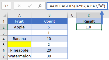
On the other hand, if we want to get the average for all cells that visually looks blank, we’ll change the criteria to be “”, and the formula looks like
=AVERAGEIFS(B2:B7,A2:A7,"")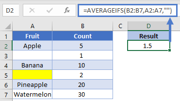
Let’s flip it around: what if you want to find the average of non-blank cells? Unfortunately, the current design won’t let you avoid the zero-length string. You can use a criterion of “<>”, but as you can see in the example, it still includes the value from row 5.
=AVERAGEIFS(B2:B7,A2:A7,"<>")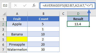
If you need to not count cells containing zero length strings, you’ll want to consider using the LEN function inside a SUMPRODUCT <link to SUMPRODUCT article).
AVERAGEIF in Google Sheets
The AVERAGEIF Function works exactly the same in Google Sheets as in Excel:
How to Use AVERAGEIF Function in Excel
Find the average for specific criteria in Excel
Updated on November 18, 2021
What to Know
- The syntax for AVERAGEIF is: =AVERAGEIF(Range,Criteria,Average_range).
- To create, select a cell, go to the Formulas tab, and select More Functions > Statistical > AVERAGEIF.
- Then enter the Range, Criteria, and Average_range in the Function dialog box and select Done.
This article explains how to use the AVERAGEIF function in Excel. Instructions apply to Excel 2019, 2016, 2013, 2010, and Excel for Microsoft 365.
What is AVERAGEIF?
The AVERAGEIF function combines the IF function and AVERAGE function in Excel; this combination allows you to find the average or arithmetic mean of those values in a selected range of data that meets specific criteria.
The IF portion of the function determines what data meets the specified criteria, while the AVERAGE part calculates the average or mean. Often, AVERAGEIF uses rows of data called records, in which all of the data in each row is related.
AVERAGEIF Function Syntax
In Excel, a function’s syntax refers to the layout of the function and includes the function’s name, brackets, and arguments.
The syntax for AVERAGEIF is:
=AVERAGEIF(Range,Criteria,Average_range)
The function’s arguments tell it what condition to test for and the range of data to average when it meets that condition.
- Range (required) is the group of cells the function will search for the specified criteria.
- Criteria (required) is the value compared against the data in the Range. You can enter actual data or the cell reference for this argument.
- Average_range (optional): The function averages the data in this range of cells when it finds matches between the Range and Criteria arguments. If you omit the Average_range argument, the function instead averages the data matched in the Range argument.
In this example, the AVERAGEIF function is looking for the average yearly sales for the East sales region. The formula will include:
- A Range of cells C3 to C9, which contains the region names.
- The Criteria is cell D12 (East).
- An Average_range of cells E3 to E9, which contains the average sales by each employee.
So if data in the range C3:C12 equals East, then the total sales for that record are averaged by the function.
Entering the AVERAGEIF Function
Although it is possible to type the AVERAGEIF function into a cell, many people find it easier to use the Function Dialog Box to add the function to a worksheet.
Begin by entering the sample data provided into cells C1 to E11 of an empty Excel worksheet as seen in the image above.
In Cell D12, under Sales Region, type East.
These instructions do not include formatting steps for the worksheet. Your worksheet will look different than the example shown, but the AVERAGE IF function will give you the same results.
-
Click on cell E12 to make it the active cell, which is where the AVERAGEIF function will go.
-
Click on the Formulas tab of the ribbon.
-
Choose More Functions > Statistical from the ribbon to open the function drop-down.
-
Click on AVERAGEIF in the list to open the Function Dialog Box. The data that goes into the three blank rows in the Function Dialog Box makes up the arguments of the AVERAGEIF function.
-
Click the Range line.
-
Highlight cells C3 to C9 in the worksheet to enter these cell references as the range to be searched by the function.
-
Click on the Criteria line.
-
Click on cell D12 to enter that cell reference — the function will search the range selected in the previous step for data that matches this criterion. Although you can input actual data – such as the word East – for this argument, it is usually more convenient to add the data to a cell in the worksheet and then input that cell reference into the dialog box.
-
Click on the Average_range line.
-
Highlight cells E3 to E9 on the spreadsheet. If the criteria specified in the previous step matches any data in the first range (C3 to C9), the function will average the data in the corresponding cells in this second range of cells.
-
Click Done to complete the AVERAGEIF function.
-
The answer $59,641 should appear in cell E12.
When you click on cell E12, the complete function appears in the formula bar above the worksheet.
= AVERAGEIF(C3:C9,D12,E3:E9)
Using a cell reference for the Criteria Argument makes it easy to find to change the criteria as needed. In this example, you can change the content of cell D12 from East to North or West. The function will automatically update and display the new result.
Thanks for letting us know!
Get the Latest Tech News Delivered Every Day
Subscribe
Answered question, solid formulas — BUT — beware of conditional averages based on numbers:
In a very similar situation I tried:
«=AVERAGE(IF(F696:F824<0;E696:E824))» (shift control enter) — In English this asked Excel to calculate an average on all numbers in column E if a result in column F was negative (a loss) — e.g. «calculate an average for all items where a loss occured». (no circular reference)
When asked to calculate an average for all items where a gain (x>0) occured, Excel got it right. However, when the conditional average was based on a loss — Excel produced a huge error (7.53 instead of 28.27).
I then opened exactly the same document in Open Office, where Calc got the (correct) answer 28,27 from the same Array formula.
Recalculating the whole thing in steps in Excel (first new column of only losses, new for only gains, new column for only E-values where a loss/gain occured, then a «clean» (unconditional) average calculation, produced the correct values.
Thus, it should be noted that Excel and Open Office produce different answers (and Excel 2007, Swedish language version, gets them wrong) in some cases of conditional averages.
(sorry for my long cautionary tale — but be a bit careful when the condition is a number would be my advice)
In this example, the goal is to calculate an average for any given group («A», «B», or «C») across all three months of data in the range C5:E16. For convenience only, data (C5:E16) and group (B5:B16) are named ranges. In the article below, we look at several approaches to this problem:
- Why the AVERAGEIFS function won’t work.
- A solution based on AVERAGE + FILTER
- A solution based on AVERAGE + IF function
- A solution based on SUMPRODUCT and Boolean algebra
In the latest version of Excel, the FILTER option (#2) is easy and intuitive. In Legacy Excel, you can use solution #3 or #4.
AVERAGEIFS won’t work
You might be tempted to solve this problem with the AVERAGEIFS function. After all, it seems to fit the bill. We simply need to calculate an average for a range of data based on one condition: we need to check if group (B5:B16) is equal to «A» or «B» or «C». In fact, we can easily use AVERAGEIFS to calculate an average for a given group on one month of data. For example, to calculate an average for group «A» in January, we can use a formula like this:
=AVERAGEIFS(C5:C16,group,"A") // returns 42However, if we try to expand average_range to include all three columns in data (C5:E16), we’ll get a #VALUE! error:
=AVERAGEIFS(data,group,"A") // returns #VALUE!Why? The reason is that AVERAGEIFS expects average_range to be the same size as criteria_range. When we try to use the 1-column range group (B5:B16) with the 3-column range data (C5:E16), AVERAGEIFS returns an error. Incidentally, if we give the older AVERAGEIF function the entire data range and the same criteria, we don’t get an error, but we do get an incorrect result:
=AVERAGEIF(group,"A",data) // returns 42This happens because AVERAGEIF makes certain assumptions about average_range, essentially resizing it to match the range argument, using the upper left cell in the range as an origin. It’s worth noting that this kind of «silent failure» is dangerous, in that the result seems reasonable but is in fact incorrect. You may not like formula errors, but at least they tell you something is wrong.
AVERAGE with FILTER
In the latest version of Excel, a good solution in this case is to use the AVERAGE function with the FILTER function. This is the approach used in the worksheet shown, where the formula in cell H5, copied down, is:
=AVERAGE(FILTER(data,group=G5))And data (C5:E16) and group (B5:B16) are named ranges. Inside the AVERAGE function, the FILTER function is configured to filter the data in C5:E16 with a simple logical expression:
FILTER(data,group=G5)Because cell G5 contains «A», and group (B5:B16) contains 12 values, the expression returns an array with 12 TRUE and FALSE values like this:
{TRUE;TRUE;TRUE;TRUE;FALSE;FALSE;FALSE;FALSE;FALSE;FALSE;FALSE;FALSE}Notice the first four values in the array are TRUE, which corresponds to the first 4 rows in the data, which are in group A. This array is returned to the FILTER function as the include argument, and FILTER uses this array to select the first 4 rows of data (C5:E16).
The result from FILTER is delivered directly to the AVERAGE function as a single array:
=AVERAGE({58,41,48;37,46,32;38,48,38;35,59,46})AVERAGE returns a final result of 43.8, the average of the 12 numbers in the array returned by FILTER. As the formula is copied down, it calculates an average for each group, using the value in column G for group.
AVERAGE with IF
The FILTER function is a newer function that does not exist in Legacy Excel. If you are using an older version of Excel, you can solve this problem with a simple array formula like this:
{=AVERAGE(IF(group=G5,data))}In this formula, we use the IF function to filter values in each group instead of FILTER. When the value in group matches the value in G5 («A»), IF returns the corresponding values in data. When a value doesn’t match, IF returns FALSE for corresponding values in data. After IF is evaluated, the array of results returned to AVERAGE looks like this:
=AVERAGE({58,41,48;37,46,32;38,48,38;35,59,46;FALSE,FALSE,FALSE;FALSE,FALSE,FALSE;FALSE,FALSE,FALSE;FALSE,FALSE,FALSE;FALSE,FALSE,FALSE;FALSE,FALSE,FALSE;FALSE,FALSE,FALSE;FALSE,FALSE,FALSE})This works because the AVERAGE function will automatically ignore the logical values TRUE and FALSE. This is an array formula and must be entered with control + shift + enter in older versions of Excel.
One thing to be aware of with this approach is that empty cells will be treated as zero, and become part of the calculated average. This happens because when the empty cells get passed through the IF function, they become zero (0). Although the AVERAGE function will ignore empty values, it will include zero (0) values in the calculated average. To avoid this problem, you can add a second IF function to test for empty values like this:
{=AVERAGE(IF(group=G5,IF(data<>"",data)))}In this formula, only values that are part of group «A» and are not empty are passed into the AVERAGE function. All other values become FALSE and are ignored by the AVERAGE function.
Both formulas above are array formulas and must be entered with control + shift + enter in older versions of Excel. In the current version of Excel, which supports array formulas natively, the formulas will «just work».
SUMPRODUCT function
As you might guess, you can also use the flexible SUMPRODUCT function to solve this problem in older versions of Excel. The formula looks like this:
=SUMPRODUCT(--(group=G5)*data)/SUMPRODUCT(--(group=G5)*(data<>""))In this formula, the first SUMPRODUCT calculates a sum of all data in group «A» (from cell G5):
=SUMPRODUCT(--(group=G5)*data) // sum (526)The second SUMPRODUCT calculates a count of all data in the same group:
SUMPRODUCT(--(group=G5)*(data<>"")) // count (12)After both SUMPRODUCT formulas are evaluated, the final step is to divide the sum by the count:
=SUMPRODUCT(--(group=G5)*data)/SUMPRODUCT(--(group=G5)*(data<>""))
=526/12
=43.8
Although slightly more complicated, the SUMPRODUCT formula does not need to be entered in a special way with control + shift + enter, since SUMPRODUCT can handle array operations natively.