
Explanation
If you want to do something specific when a cell equals a certain value, you can use the IF function to test the value, then do something if the result is TRUE, and (optionally) do something else if the result of the test is FALSE.
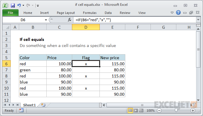
In the example shown, we want to mark rows where the color is red with an «x». In other words, we want to test cells in column B, and take a specific action when they equal the word «red». The formula in cell D6 is:
=IF(B6="red","x","")
In this formula, the logical test is this bit:
B6="red"
This will return TRUE if the value in B6 is «red» and FALSE if not. Since we want to mark or flag red items, we only need to take action when the result of the test is TRUE. In this case, we are simply adding an «x» to column D if when the color is red. If the color is not red (or blank, etc.), we simply return an empty string («»), which displays as nothing.
Note: if an empty string («») is not provided for value_if_false, the formula will return FALSE when the color is not red or green.
Increase price if color is red
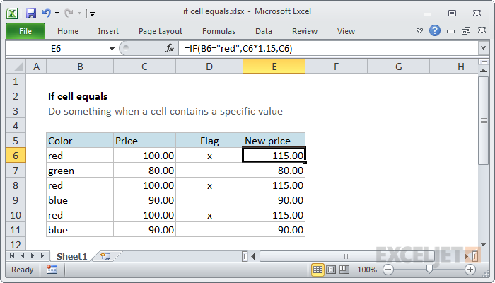
Of course, you could do something more complicated as well. For example, let’s say you want to increase the price of red items only by 15%.
In that case, you could use this formula in column E to calculate a new price:
=IF(B6="red",C6*1.15,C6)

The test is the same as before (B6=»red»). If the result is TRUE, we multiply the original price by 1.15 (increase by 15%). If the result of the test is FALSE, we simply use the original price as-is.
Содержание
- IF function
- Simple IF examples
- Common problems
- Need more help?
- How to Tell if Two Cells in Excel Contain the Same Value
- How to Check for Duplicate Cells using the Exact Function
- How to Use the Exact Excel Function to Check for Duplicates
- How to Check Excel for Duplicate Cells using the IF Function
- If cell equals
- Related functions
- Summary
- Generic formula
- Explanation
- Increase price if color is red
- Multiple cells are equal
- Related functions
- Summary
- Generic formula
- Explanation
- Case-sensitive option
- Excel: check if two cells match or multiple cells are equal
- How to check if two cells match in Excel
- If two cells equal, return TRUE
- If two cells match, return value
- If one cell equals another, then return another cell
- Case-sensitive formula to see if two cells match
- How to check if multiple cells are equal
- AND formula to see if multiple cells match
- COUNTIF formula to check if multiple columns match
- Case-sensitive formula for multiple matches
- Check if cell matches any cell in range
- Check if two ranges are equal
IF function
The IF function is one of the most popular functions in Excel, and it allows you to make logical comparisons between a value and what you expect.
So an IF statement can have two results. The first result is if your comparison is True, the second if your comparison is False.
For example, =IF(C2=”Yes”,1,2) says IF(C2 = Yes, then return a 1, otherwise return a 2).

Use the IF function, one of the logical functions, to return one value if a condition is true and another value if it’s false.
IF(logical_test, value_if_true, [value_if_false])
The condition you want to test.
The value that you want returned if the result of logical_test is TRUE.
The value that you want returned if the result of logical_test is FALSE.
Simple IF examples

In the above example, cell D2 says: IF(C2 = Yes, then return a 1, otherwise return a 2)

In this example, the formula in cell D2 says: IF(C2 = 1, then return Yes, otherwise return No)As you see, the IF function can be used to evaluate both text and values. It can also be used to evaluate errors. You are not limited to only checking if one thing is equal to another and returning a single result, you can also use mathematical operators and perform additional calculations depending on your criteria. You can also nest multiple IF functions together in order to perform multiple comparisons.
 B2,”Over Budget”,”Within Budget”)» loading=»lazy»>
=IF(C2>B2,”Over Budget”,”Within Budget”)
In the above example, the IF function in D2 is saying IF(C2 Is Greater Than B2, then return “Over Budget”, otherwise return “Within Budget”)
 B2,C2-B2,»»)» loading=»lazy»>
In the above illustration, instead of returning a text result, we are going to return a mathematical calculation. So the formula in E2 is saying IF(Actual is Greater than Budgeted, then Subtract the Budgeted amount from the Actual amount, otherwise return nothing).

In this example, the formula in F7 is saying IF(E7 = “Yes”, then calculate the Total Amount in F5 * 8.25%, otherwise no Sales Tax is due so return 0)
Note: If you are going to use text in formulas, you need to wrap the text in quotes (e.g. “Text”). The only exception to that is using TRUE or FALSE, which Excel automatically understands.
Common problems
What went wrong
There was no argument for either value_if_true or value_if_False arguments. To see the right value returned, add argument text to the two arguments, or add TRUE or FALSE to the argument.
This usually means that the formula is misspelled.
Need more help?
You can always ask an expert in the Excel Tech Community or get support in the Answers community.
Источник
How to Tell if Two Cells in Excel Contain the Same Value
Many companies still use Excel as it allows them to store different types of data, such as tax records and business contacts. Since many things are often done manually in Excel, there is a potential risk of storing duplicate information. It’s usually not an intentional act; it just happens when entering data with a typo, such as a name, account number, amount, or even an address.
Typos or misspellings often lead to new entries when existing data already exists. For instance, your records may have data for John Doe, Jon Dow, or Jon Dow, even though they are the same person.
Making these kinds of mistakes can sometimes lead to grave consequences. That’s precisely why accuracy is so important when working in spreadsheets. Thankfully, Excel includes features and tools that help everyday users check their data and correct errors.
This article shows you how to check whether two or more Excel cells have the same value.
How to Check for Duplicate Cells using the Exact Function
If you want to check whether or not two or more cells have the same value but don’t want to go through the whole table manually, you can make Excel do the work for you. Excel has a built-in function called “Exact.” This function works for both numbers and text.
How to Use the Exact Excel Function to Check for Duplicates
Let’s say you are working with the worksheet shown in the picture below. As you can see, it isn’t easy to determine whether the numbers from column A are the same as any numbers found in column B. Of course, it’s easier than comparing different cells from each column, but you get the idea.

To ensure that cells from column “A” don’t have a duplicate entry in the corresponding column “B” cells, use the “Exact” function, such as checking cells “A1” and “B1” by adding the formula to cell “C1.”
- Click on the “Formulas” tab, then select the “Text” button.

- Choose “EXACT” from the drop-down menu. The “Exact” formula works on numbers as well.
- A window called “Function Arguments” appears. You need to specify which cells you want to compare.
- To compare cells “A1” and “B1,” type “A1” in the “Text1” box and then “B1” in the “Text2” box, then click “OK.”
- Since the numbers from cells “A1” and “B1” don’t match, Excel returns a “FALSE” value and stores the result in cell “C1.”
- To check all cells, drag the “fill handle” (small square in the bottom-right corner of the cell) down the column as far as needed. This action copies and applies an adjusted formula to all other rows.
- After copying the formula down the column, you should notice that the “FALSE” value appears for non-duplicates in each row, and “TRUE” appears for identical ones.


How to Check Excel for Duplicate Cells using the IF Function
Another function that allows you to check two or more cells for duplicates is the “IF” function. It compares cells from one column, row by row. Let’s use the same two columns (A1 and B1) as in the previous example.
To use the “IF” function correctly, remember its syntax.
- In cell “C1,” type the following formula: =IF(A1=B1, “Match”, “”), and you’ll see “Match” next to the cells that have duplicate entries.
- To check for differences, you should type the following formula: =IF(A1<>B1, “No match”,” “). Again, use the fill handle by dragging it down to apply the function to all cells.
- Excel also allows you to check for duplicates and differences simultaneously by typing the following formula: =IF (A1=B1, “No Match”, “Match“) .


In closing, checking for duplicates in Excel is relatively easy when you implement formulas. The human eyes sometimes overlook identical cells, especially when there are hundreds of them to compare. Also, using formulas builds on efficiency and reduces fatigue, not to mention eye strain. These are the easiest methods to find out whether two cells have the same value in Excel.
Of course, there are times when duplicate cells are valid entries, such as dollar amounts for more than one account, two different family members with the same name, or even repeat transactions. Therefore, check the entries before taking action on them, and make a copy first to prevent data loss if something goes wrong.
Источник
If cell equals
Summary
To take one action when a cell is equal to a certain value, and another when not equal, you can use the IF function. In the example shown, the formula in cell D6 is:
Generic formula
Explanation
If you want to do something specific when a cell equals a certain value, you can use the IF function to test the value, then do something if the result is TRUE, and (optionally) do something else if the result of the test is FALSE.
In the example shown, we want to mark rows where the color is red with an «x». In other words, we want to test cells in column B, and take a specific action when they equal the word «red». The formula in cell D6 is:
In this formula, the logical test is this bit:
This will return TRUE if the value in B6 is «red» and FALSE if not. Since we want to mark or flag red items, we only need to take action when the result of the test is TRUE. In this case, we are simply adding an «x» to column D if when the color is red. If the color is not red (or blank, etc.), we simply return an empty string («»), which displays as nothing.
Note: if an empty string («») is not provided for value_if_false, the formula will return FALSE when the color is not red or green.
Increase price if color is red
Of course, you could do something more complicated as well. For example, let’s say you want to increase the price of red items only by 15%.
In that case, you could use this formula in column E to calculate a new price:
The test is the same as before (B6=»red»). If the result is TRUE, we multiply the original price by 1.15 (increase by 15%). If the result of the test is FALSE, we simply use the original price as-is.
Источник
Multiple cells are equal

Summary
To confirm two ranges of the same size contain the same values, you can use a simple array formula based on the AND function. In the example shown, the formula in C9 is:
Note: this is an array formula and must be entered with control + shift + enter.
Generic formula
Explanation
The AND function is designed to evaluate multiple logical expressions, and returns TRUE only when all expressions are TRUE.
In this case the we simply compare one range with another with a single logical expression:
The two ranges, B5:B12 and F5:H12 are the same dimensions, 5 rows x 3 columns, each containing 15 cells. The result of this operation is an array of 15 TRUE FALSE values of the same dimensions:
TRUE,TRUE,TRUE;
TRUE,TRUE,TRUE;
TRUE,TRUE,TRUE;
TRUE,TRUE,TRUE;
TRUE,TRUE,TRUE;
TRUE,TRUE,TRUE;
TRUE,TRUE,TRUE>
Each TRUE FALSE value is the result of comparing corresponding cells in the two arrays.
The AND function returns TRUE only if all values in the array are TRUE. In all other cases, AND will return FALSE.
Case-sensitive option
The formula above is not case-sensitive. To compare two ranges in a case-sensitive manner, you can use a formula like this:
Here, the EXACT function is used to make sure the test is case-sensitive. Like the formula above, this is an array formula and must be entered with control + shift + enter.
Источник
Excel: check if two cells match or multiple cells are equal
 by Alexander Frolov, updated on March 13, 2023
The tutorial will teach you how to construct the If match formula in Excel, so it returns logical values, custom text or a value from another cell.
An Excel formula to see if two cells match could be as simple as A1=B1. However, there may be different circumstances when this obvious solution won’t work or produce results different from what you expected. In this tutorial, we’ll discuss various ways to compare cells in Excel, so you can find an optimal solution for your task.
How to check if two cells match in Excel
There exist many variations of the Excel If match formula. Just review the examples below and choose the one that works best for your scenario.
If two cells equal, return TRUE
The simplest «If one cell equals another then true» Excel formula is this:
For example, to compare cells in columns A and B in each row, you enter this formula in C2, and then copy it down the column:
As the result, you’ll get TRUE if two cells are the same, FALSE otherwise:

- This formula returns two Boolean values: if two cells are equal — TRUE; if not equal — FALSE. To only return the TRUE values, use in IF statement as shown in the next example.
- This formula is case-insensitive, so it treats uppercase and lowercase letters as the same characters. If the text case matters, then use this case-sensitive formula.
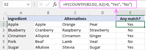
If two cells match, return value
To return your own value if two cells match, construct an IF statement using this pattern:
For example, to compare A2 and B2 and return «yes» if they contain the same values, «no» otherwise, the formula is:

If you only want to return a value if cells are equal, then supply an empty string («») for value_if_false.
If match, then yes:
If match, then TRUE:

Note. To return the logical value TRUE, don’t enclose it in double quotes. Using double quotes will convert the logical value into a regular text string.
If one cell equals another, then return another cell
And here’s a variation of the Excel if match formula that solves this specific task: compare the values in two cells and if the data match, then copy a value from another cell.
In the Excel language, it’s formulated like this:
For instance, to check the items in columns A and B and return a value from column C if text matches, the formula in D2, copied down, is:

Case-sensitive formula to see if two cells match
In situation when you are dealing with case-sensitive text values, use the EXACT function to compare the cells exactly, including the letter case:
For example, to compare the items in A2 and B2 and return «yes» if text matches exactly, «no» if any difference is found, you can use this formula:
=IF(EXACT(A2, B2), «Yes», «No»)

How to check if multiple cells are equal
As with comparing two cells, checking multiple cells for matches can also be done in a few different ways.
AND formula to see if multiple cells match
To check if multiple values match, you can use the AND function with two or more logical tests:
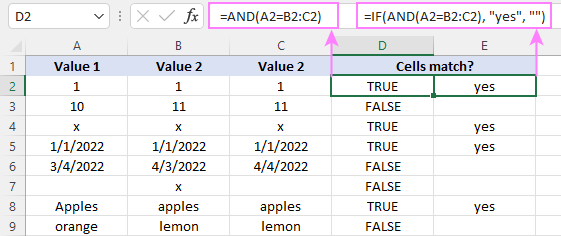
For example, to see if cells A2, B2 and C2 are equal, the formula is:
In dynamic array Excel (365 and 2021) you can also use the below syntax. In Excel 2019 and lower, this will only work as a traditional CSE array formula, completed by pressing the Ctrl + Shift + Enter keys together.
The result of both AND formulas is the logical values TRUE and FALSE.
To return your own values, wrap AND in the IF function like this:
This formula returns «yes» if all three cells are equal, a blank cell otherwise.
COUNTIF formula to check if multiple columns match
Another way to check for multiple matches is using the COUNTIF function in this form:
Where range is a range of cells to be compared against each other, cell is any single cell in the range, and n is the number of cells in the range.
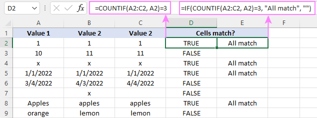
For our sample dataset, the formula can be written in this form:
If you are comparing a lot of columns, the COLUMNS function can get the cells’ count (n) for you automatically:
And the IF function will help you return anything you want as an outcome:
=IF(COUNTIF(A2:C2, A2)=3, «All match», «»)
Case-sensitive formula for multiple matches
As with checking two cells, we employ the EXACT function to perform the exact comparison, including the letter case. To handle multiple cells, EXACT is to be nested into the AND function like this:
In Excel 365 and Excel 2021, due to support for dynamic arrays, this works as a normal formula. In Excel 2019 and lower, remember to press Ctrl + Shift + Enter to make it an array formula.
For example, to check if cells A2:C2 contain the same values, a case-sensitive formula is:
In combination with IF, it takes this shape:
=IF(AND(EXACT(A2:C2, A2)), «Yes», «No»)

Check if cell matches any cell in range
To see if a cell matches any cell in a given range, utilize one of the following formulas:
It’s best to be used for checking 2 — 3 cells.
Excel 365 and Excel 2021 understand this syntax as well:
In Excel 2019 and lower, this should be entered as an array formula by pressing the Ctrl + Shift + Enter shortcut.
For instance, to check if A2 equals any cell in B2:D2, any of these formulas will do:
=OR(A2=B2, A2=C2, A2=D2)
If you are using Excel 2019 or lower, remember to press Ctrl + Shift + Enter to get the second OR formula to deliver the correct results.
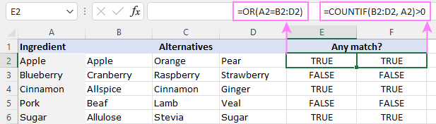
To return Yes/No or any other values you want, you know what to do — nest one of the above formulas in the logical test of the IF function. For example:
=IF(COUNTIF(B2:D2, A2)>0, «Yes», «No»)
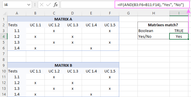
Check if two ranges are equal
To compare two ranges cell-by-cell and return the logical value TRUE if all the cells in the corresponding positions match, supply the equally sized ranges to the logical test of the AND function:
For example, to compare Matrix A in B3:F6 and Matrix B in B11:F14, the formula is:
To get Yes/No as the result, use the following IF AND combination:
=IF(AND(B3:F6=B11:F14), «Yes», «No»)
That’s how to use the If match formula in Excel. I thank you for reading and hope to see you on our blog next week!
Table of contents
Hi, I’m wanting to return a value if one cell equals another then put in say 10, otherwise leave blank. I have tried =if (d3=c3,10,””). If you leave both those cells blank it returns the 10 value which is not what I want. I want it to be blank but if those two cells are equal then I want the answer to be 10. Any help would be greatly appreciated.
To check if a cell is empty, you can use the function ISBLANK. For more information, please visit: ISBLANK function in Excel to check if cell is blank. Use the IF AND statement for multiple conditions.
If I understand your task correctly, try the following formula:
If cell 1 ,2 & 3 have values and are populated accordingly, then I want a Text string returned, for example «Matched» in a new column.
If cell 1 ,2 & 3 have no values and are not populated accordingly, then I want a Text string returned, for example «Unmatched» in a new column.
Hi!
Have you tried the ways described in this blog post? If they don’t work for you, then please describe your task in detail, explain what «populated accordingly» means.
I find a lot of this so informational! I have been scratching my head, but i’m trying to create a cell where if yes that Cell A says «Yes» based on a condition being met, and Cell B also says «Yes» on its own condition being met, that this formula will then read «Yes» indicating both conditions were met. Same if only one says YES and the other says No, this will read «no» and they must both be «YES» to end up as a yes? The issue i have is, if both cells conditions were not met and it says «no» the final cell is still indicating «true» since they match each other.
If that made sense to anyone.
Hi!
If I got you right, the formula below will help you with your task:
Wow. I am just speechless, Alexander. You are extremely skilled at this, and understand it so phenomenally! I can’t thank you enough for that!
I am comparing two columns and the individual columns have duplicated values. How can I match ? for example if one of the column have two 10,000 and the other column have three 10,000 I want to get one 10,000 as a difference.
I am working a pulling info and I was using vlookup and it work great =VLOOKUP(A2,’Employee Ben’!A$2:DE$1650,107,FALSE)
I can reference the ssn in the first column and then it searches the employee ben sheet for the number and then pulls the column that i ask for for the match. Problem is need to match 2 fields in the same row and and then pull a specified column. I cannot figure this out. Driving me Mad.
Hello!
To Vlookup multiple criteria, you can use either an INDEX MATCH combination with multiple criteria or the XLOOKUP function.
Is there a way to look at all (text) data in Column A, does it match a text value in Column B, and if ‘yes’ — enter what is in Column C into Column D.
Column B, C and D are all aligned in the same row.
hello
I want to ask if there is a possibility of compare the names in two rows where by in each row there are three for each person and the names but some of the names are not match exactly. If there is a possibility that at least two names to be match and the status became match
example
Mussa Jayden Ally vs Musa Jayden Ally
I need to see these match regardless of the difference in the name mussa vs musa
Hello!
You can split each text into 3 columns as described in this guide: How to split cells in Excel. Then compare the columns using these guidelines: Compare two columns for matches and differences.
Copyright © 2003 – 2023 Office Data Apps sp. z o.o. All rights reserved.
Microsoft and the Office logos are trademarks or registered trademarks of Microsoft Corporation. Google Chrome is a trademark of Google LLC.
Источник
This post will guide you how to check if the values of multiple cells are equal with a formula in Excel. How do I verify that multiple cellsare the same in Excel. How to compare three or more cells in Excel to see if they are the same with a formula.
Table of Contents
- Check If Multiple Cells are Equal
- Related Functions
Assuming that you have a list of data in range A1:C1, and you want to compare if these cells are equal, if so, then return True, otherwise, return False. How to achieve it.
You need to create an Excel array formula based on the AND function and the EXACT function. Just like this:
=AND(EXACT(A1:C1,A1))
Type this formula into a blank cell, and press Ctrl +Shift +Enter shortcuts in your keyboard.
There is another formula based on the COUNTIF function to achieve the same result. Like this:
=COUNTIF(A1:C1,A1)=3
- Excel AND function
The Excel AND function returns TRUE if all of arguments are TRUE, and it returns FALSE if any of arguments are FALSE.The syntax of the AND function is as below:= AND (condition1,[condition2],…) … - Excel COUNTIF function
The Excel COUNTIF function will count the number of cells in a range that meet a given criteria. This function can be used to count the different kinds of cells with number, date, text values, blank, non-blanks, or containing specific characters.etc.= COUNTIF (range, criteria)… - Excel EXACT function
The Excel EXACT function compares if two text strings are the same and returns TRUE if they are the same, Or, it will return FALSE.The syntax of the EXACT function is as below:= EXACT (text1,text2)…
Как мы все знаем, для сравнения, если две ячейки равны, мы можем использовать формулу A1 = B1. Но если вы хотите проверить, имеют ли несколько ячеек одно и то же значение, эта формула не будет работать. Сегодня я расскажу о некоторых формулах для сравнения, если несколько ячеек равны в Excel.
Сравните, если несколько ячеек равны с формулами
 Сравните, если несколько ячеек равны с формулами
Предположим, у меня есть следующий диапазон данных, теперь мне нужно знать, равны ли значения в A1: D1, для решения этой задачи вам помогут следующие формулы.
1. В пустой ячейке, помимо ваших данных, введите следующую формулу: = И (ТОЧНО (A1: D1; A1))(A1: D1 указывает ячейки, которые вы хотите сравнить, и A1 является первым значением в вашем диапазоне данных) см. снимок экрана:

2, Затем нажмите Shift + Ctrl + Enter вместе, чтобы получить результат, если значения ячеек равны, он будет отображать ИСТИНА, в противном случае будет отображаться НЕПРАВДА, см. снимок экрана:
3. И выберите ячейку, затем перетащите маркер заполнения в диапазон, который вы хотите применить к этой формуле, вы получите следующий результат:

Ноты:
1. Приведенная выше формула чувствительна к регистру.
2. Если вам нужно сравнить значения без учета регистра, вы можете применить эту формулу: = СЧЁТЕСЛИ (A1: D1; A1) = 4(A1: D1 указывает ячейки, которые вы хотите сравнить, A1 — первое значение в вашем диапазоне данных, а число 4 относится к количеству ячеек, которые вы хотите проверить), затем нажмите Enter key, и вы получите следующий результат:
Связанная статья:
Как в Excel проверить, является ли число целым?
Лучшие инструменты для работы в офисе
Kutools for Excel Решит большинство ваших проблем и повысит вашу производительность на 80%
- Снова использовать: Быстро вставить сложные формулы, диаграммы и все, что вы использовали раньше; Зашифровать ячейки с паролем; Создать список рассылки и отправлять электронные письма …
- Бар Супер Формулы (легко редактировать несколько строк текста и формул); Макет для чтения (легко читать и редактировать большое количество ячеек); Вставить в отфильтрованный диапазон…
- Объединить ячейки / строки / столбцы без потери данных; Разделить содержимое ячеек; Объединить повторяющиеся строки / столбцы… Предотвращение дублирования ячеек; Сравнить диапазоны…
- Выберите Дубликат или Уникальный Ряды; Выбрать пустые строки (все ячейки пустые); Супер находка и нечеткая находка во многих рабочих тетрадях; Случайный выбор …
- Точная копия Несколько ячеек без изменения ссылки на формулу; Автоматическое создание ссылок на несколько листов; Вставить пули, Флажки и многое другое …
- Извлечь текст, Добавить текст, Удалить по позиции, Удалить пробел; Создание и печать промежуточных итогов по страницам; Преобразование содержимого ячеек в комментарии…
- Суперфильтр (сохранять и применять схемы фильтров к другим листам); Расширенная сортировка по месяцам / неделям / дням, периодичности и др .; Специальный фильтр жирным, курсивом …
- Комбинируйте книги и рабочие листы; Объединить таблицы на основе ключевых столбцов; Разделить данные на несколько листов; Пакетное преобразование xls, xlsx и PDF…
- Более 300 мощных функций. Поддерживает Office/Excel 2007-2021 и 365. Поддерживает все языки. Простое развертывание на вашем предприятии или в организации. Полнофункциональная 30-дневная бесплатная пробная версия. 60-дневная гарантия возврата денег.
")
Вкладка Office: интерфейс с вкладками в Office и упрощение работы
- Включение редактирования и чтения с вкладками в Word, Excel, PowerPoint, Издатель, доступ, Visio и проект.
- Открывайте и создавайте несколько документов на новых вкладках одного окна, а не в новых окнах.
- Повышает вашу продуктивность на 50% и сокращает количество щелчков мышью на сотни каждый день!
")
Комментарии (40)
Оценок пока нет. Оцените первым!
Excel allows us to sum all values from a table that equal to the selected value by using the SUMIF function. This step by step tutorial will assist all levels of Excel users in summing values from the table with a certain condition.
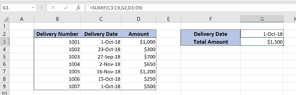 Figure 1. The final result of the SUMIF function
Syntax of the SUMIF formula
=SUMIF(range, criteria, sum_range)
The parameters of the SUMIF function are:
- range – a range of cells which we want to evaluate
- criteria – criteria for summing data
- sum_range – a range of cells that we want to sum if a condition is met
Setting up Our Data for the SUMIF Function
Our table consists of 3 columns: “Delivery Number” (column B), “Delivery Date” (column C) and “Amount” (column D). In cell G2, we specify a date for which we want to sum the amounts. In the cell G3, we want to get a sum of all amounts where a date from the column D is equal to the date in the cell G2.
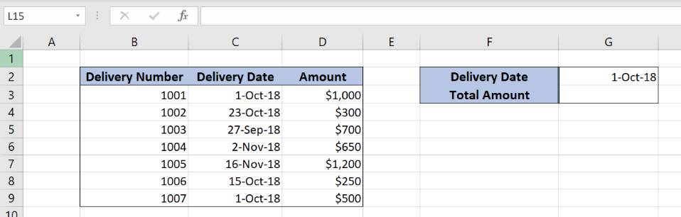 Figure 2. Data that we will use in the SUMIF example
Sum Amount if Cells are Equal to the Condition
We want to sum all amounts from column D that have appropriate date equal to 1-Oct-18.
The formula looks like:
=SUMIF(C3:C9, G2, D3:D9)
The range is C3:C9, while the criteria is G2. The sum_range is D3:D9.
To apply the SUMIFS function, we need to follow these steps:
- Select cell G3 and click on it
- Insert the formula:
=SUMIF(C3:C9,G2,D3:D9) - Press enter
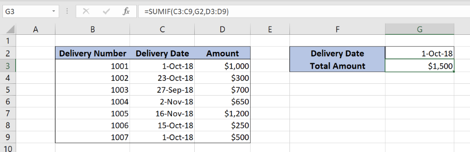 Figure 3. Using the SUMIF function to sum values greater than the limit
We see in this example that the formula sums all the amounts that have date 1-Oct-18 in the table. As you can see, rows 3($1,000) and 9($500) meet the condition, so corresponding amounts are summed. Finally, the sum in the cell G3 is $1,500.
Most of the time, the problem you will need to solve will be more complex than a simple application of a formula or function. If you want to save hours of research and frustration, try our live Excelchat service! Our Excel Experts are available 24/7 to answer any Excel question you may have. We guarantee a connection within 30 seconds and a customized solution within 20 minutes.
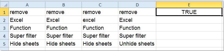
To compare the values of two or more cells there are multiple formulas that can be used. For example, MATCH, If(A=B), EXACT, COUNTIF, etc. Here we will be learning the following two functions to find the exact match or where the formula will compare the strings without considering the case of strings.
-
EXACT − To find the exact match.
-
COUNTIF − To find similar values.
Compare Multiple Cells for Equal Values
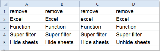
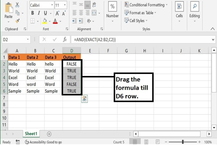
Step 1 − Following is the sample data that we have taken for comparing the strings/cell values in a datasheet.
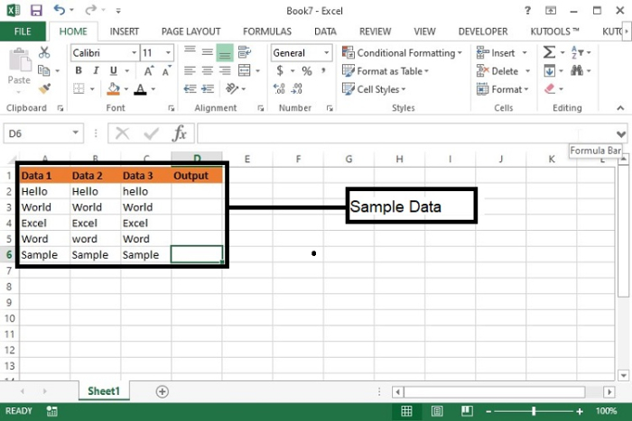
Step 2 − Here, we have taken 3 columns with some similar data and some different data. In the 4th column the output will be displayed.
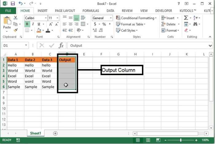
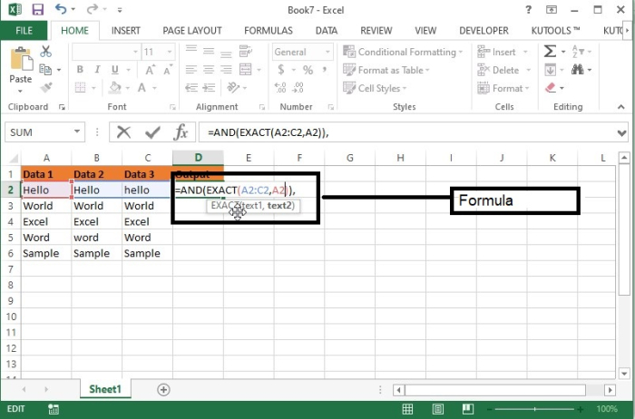
Step 3 − Enter the following formula, in D2 cell and drag the same till the row which you want to copy the formula.
=AND(EXACT(A2−C2,A2))
Here, A2−C2 indicates the range of values and A2 indicates the starting value to compare.
Formula Syntax Description
|
Argument |
Description |
|---|---|
|
IF(logical_test, {value_if_true},{value_if_false} |
|
|
Exact(Text1,Text2) |
|
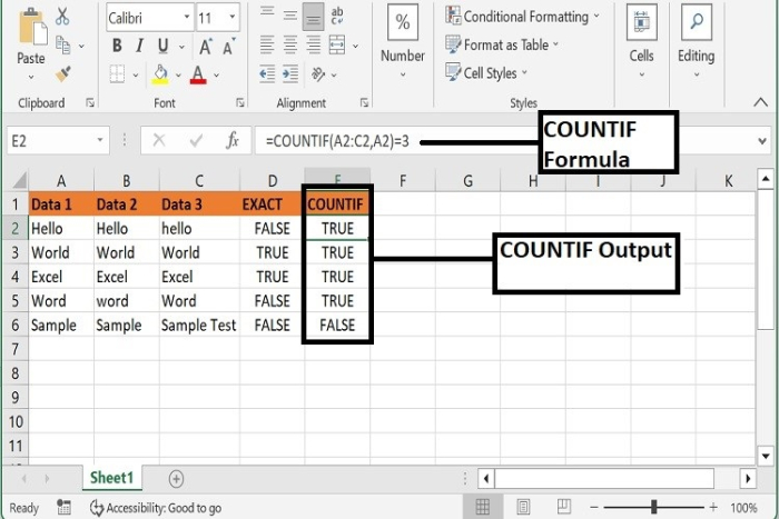
COUNTIF Formula
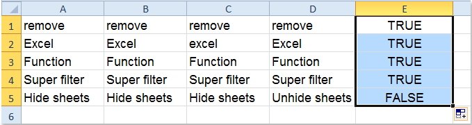
The EXACT formula return true only if the values matches exactly whereas, the COUNTIF function return TRUE if the values are similar irrespective of the case of the values. Let’s learn how to apply COUNTIF function.
Step 1 − Replace the above formula with the following function and check the output as following.
=COUNTIF(A2−C2,A2)=3
Here, A2−C2 indicates the values that need to be compared with each other and the A2 indicates the starting value. Here 3 indicates the number of values to be compared.
Conclusion
Hence, we have learned two functions to compare the multiple cell values with exact and similar value types. Keep practicing and keep learning excel.
I have three cells, any combination of which can be blank. I want to check if all non-blank cells are equal. If cells 1 and 2 have a value and cell 3 is blank, I want the formula to return TRUE if cells 1 and 2 are equal.
If there is no native formula for this then I will just write a VBA macro.
Update: It was actually quicker to just write a VBA macro. I am a .NET/c# developer and have forgotten a lot of my VBA from back in the day, so I am open for improvements on my code here (especially setting the return value and exiting the function).
Public Function NonblankValuesAreEqual(cells As Range) As Boolean

Dim lastval As String

lastval = cells(1).Value

For i = 2 To cells.Count
    If lastval <> "" Then
        If cells(i).Value <> "" Then
            If cells(i).Value <> lastval Then
                NonblankValuesAreEqual = False
                Exit Function
            End If
        End If
    End If
    lastval = cells(i).Value
Next

NonblankValuesAreEqual = True

End Function
asked Sep 30, 2015 at 13:43
![]()
oscilatingcretinoscilatingcretin
5,00325 gold badges77 silver badges115 bronze badges
2
You’ve already answered yourself with a macro, but here is a non-VBA solution. It’s an array formula, and must be confirmed with ctrl+shift+enter:
=(SUM(IFERROR(1/COUNTIF(A1:A3,A1:A3),0))=1)
This formula counts the number of unique values in your range, while ignoring blank cells. If the number of unique values is 1, then every value is the same and the formula returns TRUE. The only thing that wasn’t specified in your question is what to do if every cell is blank. Right now the formula will return TRUE, but it would be easy to add some additional logic to change that.
answered Sep 30, 2015 at 14:56
![]()
KyleKyle
2,4062 gold badges10 silver badges12 bronze badges
4
Check if each column-pair exactly equal (case-sensitive) or contain a blank.
=OR(EXACT(A2,B2),ISBLANK(A2),ISBLANK(B2))
=OR(EXACT(A2,C2),ISBLANK(A2),ISBLANK(C2))
=OR(EXACT(B2,C2),ISBLANK(B2),ISBLANK(C2))

=AND(D2:F2)
Example:
A   B   C   AB      AC      BC      AND
1   1   1   TRUE    TRUE    TRUE    TRUE
1   1       TRUE    TRUE    TRUE    TRUE
A           TRUE    TRUE    TRUE    TRUE
    A       TRUE    TRUE    TRUE    TRUE
        A   TRUE    TRUE    TRUE    TRUE
a   A   a   FALSE   TRUE    FALSE   FALSE
a   a       TRUE    TRUE    TRUE    TRUE
a       2   TRUE    FALSE   TRUE    FALSE
    A   A   TRUE    TRUE    TRUE    TRUE
A       A   TRUE    TRUE    TRUE    TRUE
    A   B   TRUE    TRUE    FALSE   FALSE
A   B   C   FALSE   FALSE   FALSE   FALSE
Note: For larger sets, the number of adjacent columns will increase greatly: n! / 2
answered Sep 30, 2015 at 13:49
![]()
StevenSteven
27.3k11 gold badges95 silver badges117 bronze badges
2
Try this small UDF():
Public Function EqualTest(r1 As Range, r2 As Range, r3 As Range) As Variant
   Dim BlankCount As Long, v1 As Variant, v2 As Variant, v3 As Variant
   v1 = r1.Value
   v2 = r2.Value
   v3 = r3.Value
   BlankCount = 0
   If v1 = "" Then BlankCount = BlankCount + 1
   If v2 = "" Then BlankCount = BlankCount + 1
   If v3 = "" Then BlankCount = BlankCount + 1

   If BlankCount > 1 Then
      EqualTest = True
      Exit Function
   End If

   If BlankCount = 0 Then
      If v1 = v2 And v1 = v3 And v2 = v3 Then
         EqualTest = True
         Exit Function
      Else
         EqualTest = False
         Exit Function
      End If
   End If

   If v1 = v2 Or v1 = v3 Or v2 = v3 Then
      EqualTest = True
   Else
      EqualTest = False
   End If
End Function

NOTE:
The cells do not have to be contiguous and the UDF() will work for both numeric cells and text cells.
answered Sep 30, 2015 at 14:16
![]()
Gary’s StudentGary’s Student
19.2k6 gold badges25 silver badges38 bronze badges
4
Try:
=COUNTA(A:A)=COUNTIF(A:A,A1)
Basically count the number of nonblank cells.
Count the number of cells matching the first cell.
If those are the same, then they must all be the same.
It doesn’t really matter who you count for the 2nd COUNTIF … since it won’t likely be equal to COUNTA if they aren’t all the same 
[edit]
if your first cell could be blank .. try this instead:
=COUNTA(A:A)=COUNTIF(A:A,VLOOKUP("*",A:A,1,FALSE))
it’ll try to find the first non-blank cell to check in the COUNTIF ..
answered Sep 30, 2015 at 14:00
![]()
DittoDitto
1902 silver badges11 bronze badges
2
I have multiple tables that use the same ID values but have different items and descriptions assigned to them. The ID order is fixed and same in all tables.
What I’d like to do is find out which table rows are the same across all tables.
     A  B  C     D  E  F     G  H  I

1    H1 H2 H3    H1 H2 H3    H1 H2 H3
     -- -- --    -- -- --    -- -- --
2    1  a  a+    1  a  a+    1  c  c+    FALSE
3    2  b  b+    2  b  b+    2  b  b+    TRUE
4    3  c  c+    3  x  x+    3  a  a+    FALSE

H1 = ID, same values and order in all tables
H2 = item; order varies by table
H3 = item description; items & descriptions come in fixed pairs
What I’ve done so far is placed them next to each other, and I’m using the following formula in the last column:
=SUMPRODUCT(ABS(COUNTIF(A2:I2; A2:I2) - 3)) = 0
-
COUNTIFreturns the array of the entire multi-table row containing the number of occurrences of each cell’s value within that same row. For the three tables in the example, that will be three dupes of each cell per row, or[3,3,3, 3,3,3, 3,3,3]. -
The
-3part zeroes out the array,[0,0,0, 0,0,0, 0,0,0], for rows with matching table values. -
ABSdrops the minuses from any potential negative numbers in the array caused by the previous step. This makes sure that, in the last step, only the sums of duped-row arrays can equal zero, while all the other arrays will result in a value >0. -
SUMPRODUCTsums the array and returns a single value that can then be compared to zero, which the second step has assured means that all the tables’ values in the current row match. (Actually, a simpleSUMis a more straightforward choice, but for some reason, unlikeSUMPRODUCT, it requires Ctrl+Shift+Enter when entering the formula).
Is there a simpler formula or layout I can use to deal with this problem?