
The IF function allows you to make a logical comparison between a value and what you expect by testing for a condition and returning a result if that condition is True or False.
-
=IF(Something is True, then do something, otherwise do something else)
But what if you need to test multiple conditions, where let’s say all conditions need to be True or False (AND), or only one condition needs to be True or False (OR), or if you want to check if a condition does NOT meet your criteria? All 3 functions can be used on their own, but it’s much more common to see them paired with IF functions.
Use the IF function along with AND, OR and NOT to perform multiple evaluations if conditions are True or False.
Syntax
-
IF(AND()) — IF(AND(logical1, [logical2], …), value_if_true, [value_if_false]))
-
IF(OR()) — IF(OR(logical1, [logical2], …), value_if_true, [value_if_false]))
-
IF(NOT()) — IF(NOT(logical1), value_if_true, [value_if_false]))
|
Argument name |
Description |
|
|
logical_test (required) |
The condition you want to test. |
|
|
value_if_true (required) |
The value that you want returned if the result of logical_test is TRUE. |
|
|
value_if_false (optional) |
The value that you want returned if the result of logical_test is FALSE. |
|
Here are overviews of how to structure AND, OR and NOT functions individually. When you combine each one of them with an IF statement, they read like this:
-
AND – =IF(AND(Something is True, Something else is True), Value if True, Value if False)
-
OR – =IF(OR(Something is True, Something else is True), Value if True, Value if False)
-
NOT – =IF(NOT(Something is True), Value if True, Value if False)
Examples
Following are examples of some common nested IF(AND()), IF(OR()) and IF(NOT()) statements. The AND and OR functions can support up to 255 individual conditions, but it’s not good practice to use more than a few because complex, nested formulas can get very difficult to build, test and maintain. The NOT function only takes one condition.

Here are the formulas spelled out according to their logic:
|
Formula |
Description |
|---|---|
|
=IF(AND(A2>0,B2<100),TRUE, FALSE) |
IF A2 (25) is greater than 0, AND B2 (75) is less than 100, then return TRUE, otherwise return FALSE. In this case both conditions are true, so TRUE is returned. |
|
=IF(AND(A3=»Red»,B3=»Green»),TRUE,FALSE) |
If A3 (“Blue”) = “Red”, AND B3 (“Green”) equals “Green” then return TRUE, otherwise return FALSE. In this case only the first condition is true, so FALSE is returned. |
|
=IF(OR(A4>0,B4<50),TRUE, FALSE) |
IF A4 (25) is greater than 0, OR B4 (75) is less than 50, then return TRUE, otherwise return FALSE. In this case, only the first condition is TRUE, but since OR only requires one argument to be true the formula returns TRUE. |
|
=IF(OR(A5=»Red»,B5=»Green»),TRUE,FALSE) |
IF A5 (“Blue”) equals “Red”, OR B5 (“Green”) equals “Green” then return TRUE, otherwise return FALSE. In this case, the second argument is True, so the formula returns TRUE. |
|
=IF(NOT(A6>50),TRUE,FALSE) |
IF A6 (25) is NOT greater than 50, then return TRUE, otherwise return FALSE. In this case 25 is not greater than 50, so the formula returns TRUE. |
|
=IF(NOT(A7=»Red»),TRUE,FALSE) |
IF A7 (“Blue”) is NOT equal to “Red”, then return TRUE, otherwise return FALSE. |
Note that all of the examples have a closing parenthesis after their respective conditions are entered. The remaining True/False arguments are then left as part of the outer IF statement. You can also substitute Text or Numeric values for the TRUE/FALSE values to be returned in the examples.
Here are some examples of using AND, OR and NOT to evaluate dates.

Here are the formulas spelled out according to their logic:
|
Formula |
Description |
|---|---|
|
=IF(A2>B2,TRUE,FALSE) |
IF A2 is greater than B2, return TRUE, otherwise return FALSE. 03/12/14 is greater than 01/01/14, so the formula returns TRUE. |
|
=IF(AND(A3>B2,A3<C2),TRUE,FALSE) |
IF A3 is greater than B2 AND A3 is less than C2, return TRUE, otherwise return FALSE. In this case both arguments are true, so the formula returns TRUE. |
|
=IF(OR(A4>B2,A4<B2+60),TRUE,FALSE) |
IF A4 is greater than B2 OR A4 is less than B2 + 60, return TRUE, otherwise return FALSE. In this case the first argument is true, but the second is false. Since OR only needs one of the arguments to be true, the formula returns TRUE. If you use the Evaluate Formula Wizard from the Formula tab you’ll see how Excel evaluates the formula. |
|
=IF(NOT(A5>B2),TRUE,FALSE) |
IF A5 is not greater than B2, then return TRUE, otherwise return FALSE. In this case, A5 is greater than B2, so the formula returns FALSE. |

Using AND, OR and NOT with Conditional Formatting
You can also use AND, OR and NOT to set Conditional Formatting criteria with the formula option. When you do this you can omit the IF function and use AND, OR and NOT on their own.
From the Home tab, click Conditional Formatting > New Rule. Next, select the “Use a formula to determine which cells to format” option, enter your formula and apply the format of your choice.

Using the earlier Dates example, here is what the formulas would be.

|
Formula |
Description |
|---|---|
|
=A2>B2 |
If A2 is greater than B2, format the cell, otherwise do nothing. |
|
=AND(A3>B2,A3<C2) |
If A3 is greater than B2 AND A3 is less than C2, format the cell, otherwise do nothing. |
|
=OR(A4>B2,A4<B2+60) |
If A4 is greater than B2 OR A4 is less than B2 plus 60 (days), then format the cell, otherwise do nothing. |
|
=NOT(A5>B2) |
If A5 is NOT greater than B2, format the cell, otherwise do nothing. In this case A5 is greater than B2, so the result will return FALSE. If you were to change the formula to =NOT(B2>A5) it would return TRUE and the cell would be formatted. |
Note: A common error is to enter your formula into Conditional Formatting without the equals sign (=). If you do this you’ll see that the Conditional Formatting dialog will add the equals sign and quotes to the formula — =»OR(A4>B2,A4<B2+60)», so you’ll need to remove the quotes before the formula will respond properly.
Need more help?

See also
You can always ask an expert in the Excel Tech Community or get support in the Answers community.
Learn how to use nested functions in a formula
IF function
AND function
OR function
NOT function
Overview of formulas in Excel
How to avoid broken formulas
Detect errors in formulas
Keyboard shortcuts in Excel
Logical functions (reference)
Excel functions (alphabetical)
Excel functions (by category)
Функция ЕСЛИ в Excel — это отличный инструмент для проверки условий на ИСТИНУ или ЛОЖЬ. Если значения ваших расчетов равны заданным параметрам функции как ИСТИНА, то она возвращает одно значение, если ЛОЖЬ, то другое.
Содержание
- Что возвращает функция
- Синтаксис
- Аргументы функции
- Дополнительная информация
- Функция Если в Excel примеры с несколькими условиями
- Пример 1. Проверяем простое числовое условие с помощью функции IF (ЕСЛИ)
- Пример 2. Использование вложенной функции IF (ЕСЛИ) для проверки условия выражения
- Пример 3. Вычисляем сумму комиссии с продаж с помощью функции IF (ЕСЛИ) в Excel
- Пример 4. Используем логические операторы (AND/OR) (И/ИЛИ) в функции IF (ЕСЛИ) в Excel
- Пример 5. Преобразуем ошибки в значения “0” с помощью функции IF (ЕСЛИ)
Что возвращает функция
Заданное вами значение при выполнении двух условий ИСТИНА или ЛОЖЬ.
Синтаксис
=IF(logical_test, [value_if_true], [value_if_false]) — английская версия
=ЕСЛИ(лог_выражение; [значение_если_истина]; [значение_если_ложь]) — русская версия
Аргументы функции
- logical_test (лог_выражение) — это условие, которое вы хотите протестировать. Этот аргумент функции должен быть логичным и определяемым как ЛОЖЬ или ИСТИНА. Аргументом может быть как статичное значение, так и результат функции, вычисления;
- [value_if_true] ([значение_если_истина]) — (не обязательно) — это то значение, которое возвращает функция. Оно будет отображено в случае, если значение которое вы тестируете соответствует условию ИСТИНА;
- [value_if_false] ([значение_если_ложь]) — (не обязательно) — это то значение, которое возвращает функция. Оно будет отображено в случае, если условие, которое вы тестируете соответствует условию ЛОЖЬ.
Дополнительная информация
- В функции ЕСЛИ может быть протестировано 64 условий за один раз;
- Если какой-либо из аргументов функции является массивом — оценивается каждый элемент массива;
- Если вы не укажете условие аргумента FALSE (ЛОЖЬ) value_if_false (значение_если_ложь) в функции, т.е. после аргумента value_if_true (значение_если_истина) есть только запятая (точка с запятой), функция вернет значение “0”, если результат вычисления функции будет равен FALSE (ЛОЖЬ).
На примере ниже, формула =IF(A1> 20,”Разрешить”) или =ЕСЛИ(A1>20;»Разрешить») , где value_if_false (значение_если_ложь) не указано, однако аргумент value_if_true (значение_если_истина) по-прежнему следует через запятую. Функция вернет “0” всякий раз, когда проверяемое условие не будет соответствовать условиям TRUE (ИСТИНА).
 |
| - Если вы не укажете условие аргумента TRUE(ИСТИНА) (value_if_true (значение_если_истина)) в функции, т.е. условие указано только для аргумента value_if_false (значение_если_ложь), то формула вернет значение “0”, если результат вычисления функции будет равен TRUE (ИСТИНА);
На примере ниже формула равна =IF (A1>20;«Отказать») или =ЕСЛИ(A1>20;»Отказать»), где аргумент value_if_true (значение_если_истина) не указан, формула будет возвращать “0” всякий раз, когда условие соответствует TRUE (ИСТИНА).

Функция Если в Excel примеры с несколькими условиями
Пример 1. Проверяем простое числовое условие с помощью функции IF (ЕСЛИ)
При использовании функции ЕСЛИ в Excel, вы можете использовать различные операторы для проверки состояния. Вот список операторов, которые вы можете использовать:
Ниже приведен простой пример использования функции при расчете оценок студентов. Если сумма баллов больше или равна «35», то формула возвращает “Сдал”, иначе возвращается “Не сдал”.
Пример 2. Использование вложенной функции IF (ЕСЛИ) для проверки условия выражения
Функция может принимать до 64 условий одновременно. Несмотря на то, что создавать длинные вложенные функции нецелесообразно, то в редких случаях вы можете создать формулу, которая множество условий последовательно.
В приведенном ниже примере мы проверяем два условия.
- Первое условие проверяет, сумму баллов не меньше ли она чем 35 баллов. Если это ИСТИНА, то функция вернет “Не сдал”;
- В случае, если первое условие — ЛОЖЬ, и сумма баллов больше 35, то функция проверяет второе условие. В случае если сумма баллов больше или равна 75. Если это правда, то функция возвращает значение “Отлично”, в других случаях функция возвращает “Сдал”.
Пример 3. Вычисляем сумму комиссии с продаж с помощью функции IF (ЕСЛИ) в Excel
Функция позволяет выполнять вычисления с числами. Хороший пример использования — расчет комиссии продаж для торгового представителя.
В приведенном ниже примере, торговый представитель по продажам:
- не получает комиссионных, если объем продаж меньше 50 тыс;
- получает комиссию в размере 2%, если продажи между 50-100 тыс
- получает 4% комиссионных, если объем продаж превышает 100 тыс.
Рассчитать размер комиссионных для торгового агента можно по следующей формуле:
=IF(B2<50,0,IF(B2<100,B2*2%,B2*4%)) — английская версия
=ЕСЛИ(B2<50;0;ЕСЛИ(B2<100;B2*2%;B2*4%)) — русская версия
В формуле, использованной в примере выше, вычисление суммы комиссионных выполняется в самой функции ЕСЛИ. Если объем продаж находится между 50-100K, то формула возвращает B2 * 2%, что составляет 2% комиссии в зависимости от объема продажи.
Больше лайфхаков в нашем Telegram Подписаться
Пример 4. Используем логические операторы (AND/OR) (И/ИЛИ) в функции IF (ЕСЛИ) в Excel
Вы можете использовать логические операторы (AND/OR) (И/ИЛИ) внутри функции для одновременного тестирования нескольких условий.
Например, предположим, что вы должны выбрать студентов для стипендий, основываясь на оценках и посещаемости. В приведенном ниже примере учащийся имеет право на участие только в том случае, если он набрал более 80 баллов и имеет посещаемость более 80%.
Вы можете использовать функцию AND (И) вместе с функцией IF (ЕСЛИ), чтобы сначала проверить, выполняются ли оба эти условия или нет. Если условия соблюдены, функция возвращает “Имеет право”, в противном случае она возвращает “Не имеет право”.
Формула для этого расчета:
=IF(AND(B2>80,C2>80%),”Да”,”Нет”) — английская версия
=ЕСЛИ(И(B2>80;C2>80%);»Да»;»Нет») — русская версия
Пример 5. Преобразуем ошибки в значения “0” с помощью функции IF (ЕСЛИ)
С помощью этой функции вы также можете убирать ячейки содержащие ошибки. Вы можете преобразовать значения ошибок в пробелы или нули или любое другое значение.
Формула для преобразования ошибок в ячейках следующая:
=IF(ISERROR(A1),0,A1) — английская версия
=ЕСЛИ(ЕОШИБКА(A1);0;A1) — русская версия
Формула возвращает “0”, в случае если в ячейке есть ошибка, иначе она возвращает значение ячейки.
ПРИМЕЧАНИЕ. Если вы используете Excel 2007 или версии после него, вы также можете использовать функцию IFERROR для этого.
Точно так же вы можете обрабатывать пустые ячейки. В случае пустых ячеек используйте функцию ISBLANK, на примере ниже:
=IF(ISBLANK(A1),0,A1) — английская версия
=ЕСЛИ(ЕПУСТО(A1);0;A1) — русская версия
The IF function runs a logical test and returns one value for a TRUE result, and another value for a FALSE result. The result from IF can be a value, a cell reference, or even another formula. By combining the IF function with other logical functions like AND and OR, you can test more than one condition at a time.
Syntax
The generic syntax for the IF function looks like this:
=IF(logical_test,[value_if_true],[value_if_false])The first argument, logical_test, is typically an expression that returns either TRUE or FALSE. The second argument, value_if_true, is the value to return when logical_test is TRUE. The last argument, value_if_false, is the value to return when logical_test is FALSE. Both value_if_true and value_if_false are optional, but you must provide one or the other. For example, if cell A1 contains 80, then:
=IF(A1>75,TRUE) // returns TRUE
=IF(A1>75,"OK") // returns "OK"
=IF(A1>85,"OK") // returns FALSE
=IF(A1>75,10,0) // returns 10
=IF(A1>85,10,0) // returns 0
=IF(A1>75,"Yes","No") // returns "Yes"
=IF(A1>85,"Yes","No") // returns "No"
Notice that text values like «OK», «Yes», «No», etc. must be enclosed in double quotes («»). However, numeric values should not be enclosed in quotes.
Logical tests
The IF function supports logical operators (>,<,<>,=) when creating logical tests. Most commonly, the logical_test in IF is a complete logical expression that will evaluate to TRUE or FALSE. The table below shows some common examples:
| Goal | Logical test |
|---|---|
| If A1 is greater than 75 | A1>75 |
| If A1 equals 100 | A1=100 |
| If A1 is less than or equal to 100 | A1<=100 |
| If A1 equals «Red» | A1=»red» |
| If A1 is not equal to «Red» | A1<>»red» |
| If A1 is less than B1 | A1<B1 |
| If A1 is empty | A1=»» |
| If A1 is not empty | A1<>»» |
| If A1 is less than current date | A1<TODAY() |
Notice text values must be enclosed in double quotes («»), but numbers do not. The IF function does not support wildcards, but you can combine IF with COUNTIF to get basic wildcard functionality. To test for substrings in a cell, you can use the IF function with the SEARCH function.
Pass or Fail example
In the worksheet shown above, we want to assign either «Pass» or «Fail» based on a test score. A passing score is 70 or higher. The formula in D6, copied down, is:
=IF(C5>=70,"Pass","Fail")
Translation: If the value in C5 is greater than or equal to 70, return «Pass». Otherwise, return «Fail».
Note that the logical flow of this formula can be reversed. This formula returns the same result:
=IF(C5<70,"Fail","Pass")
Translation: If the value in C5 is less than 70, return «Fail». Otherwise, return «Pass».
Both formulas above, when copied down, will return correct results.
Note: If you are new to the idea of formula criteria, this article explains many examples.
Assign points based on color
In the worksheet below, we want to assign points based on the color in column B. If the color is «red», the result should be 100. If the color is «blue», the result should be 125. This requires that we use a formula based on two IF functions, one nested inside the other. The formula in C5, copied down, is:
=IF(B5="red",100,IF(B5="blue",125))
Translation: IF the value in B5 is «red», return 100. Else, if the value in B5 is «blue», return 125.

There are three things to notice in this example:
- The formula will return FALSE if the value in B5 is anything except «red» or «blue»
- The text values «red» and «blue» must be enclosed in double quotes («»)
- The IF function is not case-sensitive and will match «red», «Red», «RED», or «rEd».
This is a simple example of a nested IFs formula. See below for a more complex example.
Return another formula
The IF function can return another formula as a result. For example, the formula below will return A1*5% when A1 is less than 100, and A1*7% when A1 is greater than or equal to 100:
=IF(A1<100,A1*5%,A1*7%)
Nested IF statements
The IF function can be «nested». A «nested IF» refers to a formula where at least one IF function is nested inside another in order to test for more conditions and return more possible results. Each IF statement needs to be carefully «nested» inside another so that the logic is correct. For example, the following formula can be used to assign a grade rather than a pass / fail result:
=IF(C6<70,"F",IF(C6<75,"D",IF(C6<85,"C",IF(C6<95,"B","A"))))
Up to 64 IF functions can be nested. However, in general, you should consider other functions, like VLOOKUP or XLOOKUP for more complex scenarios, because they can handle more conditions in a more streamlined fashion. For a more details see this article on nested IFs.
Note: the newer IFS function is designed to handle multiple conditions without nesting. However, a lookup function like VLOOKUP or XLOOKUP is usually a better approach unless the logic for each condition is custom.
IF with AND, OR, NOT
The IF function can be combined with the AND function and the OR function. For example, to return «OK» when A1 is between 7 and 10, you can use a formula like this:
=IF(AND(A1>7,A1<10),"OK","")
Translation: if A1 is greater than 7 and less than 10, return «OK». Otherwise, return nothing («»).
To return B1+10 when A1 is «red» or «blue» you can use the OR function like this:
=IF(OR(A1="red",A1="blue"),B1+10,B1)
Translation: if A1 is red or blue, return B1+10, otherwise return B1.
=IF(NOT(A1="red"),B1+10,B1)
Translation: if A1 is NOT red, return B1+10, otherwise return B1.
IF cell contains specific text
Because the IF function does not support wildcards, it is not obvious how to configure IF to check for a specific substring in a cell. A common approach is to combine the ISNUMBER function and the SEARCH function to create a logical test like this:
=ISNUMBER(SEARCH(substring,A1)) // returns TRUE or FALSEFor example, to check for the substring «xyz» in cell A1, you can use a formula like this:
=IF(ISNUMBER(SEARCH("xyz",A1)),"Yes","No")Read a detailed explanation here.
More information
- Read more about nested IFs
- Learn how to use VLOOKUP instead of nested IFs (video)
- 50 Examples of formula criteria
Notes
- The IF function is not case-sensitive.
- To count values conditionally, use the COUNTIF or the COUNTIFS functions.
- To sum values conditionally, use the SUMIF or the SUMIFS functions.
- If any of the arguments to IF are supplied as arrays, the IF function will evaluate every element of the array.
Содержание
- Что возвращает функция
- Формула ЕСЛИ в Excel – примеры нескольких условий
- Синтаксис функции ЕСЛИ
- Расширение функционала с помощью операторов «И» и «ИЛИ»
- Простейший пример применения.
- Применение «ЕСЛИ» с несколькими условиями
- Операторы сравнения чисел и строк
- Одновременное выполнение двух условий
- Общее определение и задачи
- Как правильно записать?
- Дополнительная информация
- Вложенные условия с математическими выражениями.
- Аргументы функции
- А если один из параметров не заполнен?
- Функция ЕПУСТО
- Функции ИСТИНА и ЛОЖЬ
- Составное условие
- Простое условие
- Пример функции с несколькими условиями
- Пример использования «ЕСЛИ»
- Проверяем простое числовое условие с помощью функции IF (ЕСЛИ)
- Заключение
Что возвращает функция
Заданное вами значение при выполнении двух условий ИСТИНА или ЛОЖЬ.
Довольно часто количество возможных условий не 2 (проверяемое и альтернативное), а 3, 4 и более. В этом случае также можно использовать функцию ЕСЛИ, но теперь ее придется вкладывать друг в друга, указывая все условия по очереди. Рассмотрим следующий пример.
Нескольким менеджерам по продажам нужно начислить премию в зависимости от выполнения плана продаж. Система мотивации следующая. Если план выполнен менее, чем на 90%, то премия не полагается, если от 90% до 95% — премия 10%, от 95% до 100% — премия 20% и если план перевыполнен, то 30%. Как видно здесь 4 варианта. Чтобы их указать в одной формуле потребуется следующая логическая структура. Если выполняется первое условие, то наступает первый вариант, в противном случае, если выполняется второе условие, то наступает второй вариант, в противном случае если… и т.д. Количество условий может быть довольно большим. В конце формулы указывается последний альтернативный вариант, для которого не выполняется ни одно из перечисленных ранее условий (как третье поле в обычной формуле ЕСЛИ). В итоге формула имеет следующий вид.

Комбинация функций ЕСЛИ работает так, что при выполнении какого-либо указанно условия следующие уже не проверяются. Поэтому важно их указать в правильной последовательности. Если бы мы начали проверку с B2<1, то условия B2<0,9 и B2<0,95 Excel бы просто «не заметил», т.к. они входят в интервал B2<1 который проверился бы первым (если значение менее 0,9, само собой, оно также меньше и 1). И тогда у нас получилось бы только два возможных варианта: менее 1 и альтернативное, т.е. 1 и более.
При написании формулы легко запутаться, поэтому рекомендуется смотреть на всплывающую подсказку.

В конце нужно обязательно закрыть все скобки, иначе эксель выдаст ошибку

Синтаксис функции ЕСЛИ
Вот как выглядит синтаксис этой функции и её аргументы:
=ЕСЛИ(логическое выражение, значение если «да», значение если «нет»)
Логическое выражение – (обязательное) условие, которое возвращает значение «истина» или «ложь» («да» или «нет»);
Значение если «да» – (обязательное) действие, которое выполняется в случае положительного ответа;
Значение если «нет» – (обязательное) действие, которое выполняется в случае отрицательного ответа;
Давайте вместе подробнее рассмотрим эти аргументы.
Первый аргумент – это логический вопрос. И ответ этот может быть только «да» или «нет», «истина» или «ложь».
Как правильно задать вопрос? Для этого можно составить логическое выражение, используя знаки “=”, “>”, “<”, “>=”, “<=”, “<>”.
Расширение функционала с помощью операторов «И» и «ИЛИ»
Когда нужно проверить несколько истинных условий, используется функция И. Суть такова: ЕСЛИ а = 1 И а = 2 ТОГДА значение в ИНАЧЕ значение с.
Функция ИЛИ проверяет условие 1 или условие 2. Как только хотя бы одно условие истинно, то результат будет истинным. Суть такова: ЕСЛИ а = 1 ИЛИ а = 2 ТОГДА значение в ИНАЧЕ значение с.
Функции И и ИЛИ могут проверить до 30 условий.
Пример использования оператора И:

Пример использования функции ИЛИ:

Простейший пример применения.
Предположим, вы работаете в компании, которая занимается продажей шоколада в нескольких регионах и работает с множеством покупателей.
Нам необходимо выделить продажи, которые произошли в нашем регионе, и те, которые были сделаны за рубежом. Для этого нужно добавить в таблицу ещё один признак для каждой продажи – страну, в которой она произошла. Мы хотим, чтобы этот признак создавался автоматически для каждой записи (то есть, строки).
В этом нам поможет функция ЕСЛИ. Добавим в таблицу данных столбец “Страна”. Регион “Запад” – это местные продажи («Местные»), а остальные регионы – это продажи за рубеж («Экспорт»).
Применение «ЕСЛИ» с несколькими условиями
Мы только что рассмотрели пример использования оператора «ЕСЛИ» с одним логическим выражением. Но в программе также имеется возможность задавать больше одного условия. При этом сначала будет проводиться проверка по первому, и в случае его успешного выполнения сразу отобразится заданное значение. И только если не будет выполнено первое логическое выражение, в силу вступит проверка по второму.
Рассмотрим наглядно на примере все той же таблицы. Но на этот раз усложним задачу. Теперь нужно проставить скидку на женскую обувь в зависимости от вида спорта.
Первое условия – это проверка пола. Если “мужской” – сразу выводится значение 0. Если же это “женский”, то начинается проверка по второму условию. Если вид спорта бег – 20%, если теннис – 10%.
Пропишем формулу для этих условий в нужной нам ячейке.
=ЕСЛИ(B2=”мужской”;0; ЕСЛИ(C2=”бег”;20%;10%))

Щелкаем Enter и получаем результат согласно заданным условиям.

Далее растягиваем формулу на все оставшиеся строки таблицы.

Операторы сравнения чисел и строк
Операторы сравнения чисел и строк представлены операторами, состоящими из одного или двух математических знаков равенства и неравенства:
- < – меньше;
- <= – меньше или равно;
- > – больше;
- >= – больше или равно;
- = – равно;
- <> – не равно.
Синтаксис:
|
Результат = Выражение1 Оператор Выражение2 |
- Результат – любая числовая переменная;
- Выражение – выражение, возвращающее число или строку;
- Оператор – любой оператор сравнения чисел и строк.
Если переменная Результат будет объявлена как Boolean (или Variant), она будет возвращать значения False и True. Числовые переменные других типов будут возвращать значения 0 (False) и -1 (True).
Операторы сравнения чисел и строк работают с двумя числами или двумя строками. При сравнении числа со строкой или строки с числом, VBA Excel сгенерирует ошибку Type Mismatch (несоответствие типов данных):
|
Sub Primer1() On Error GoTo Instr Dim myRes As Boolean ‘Сравниваем строку с числом myRes = “пять” > 3 Instr: If Err.Description <> “” Then MsgBox “Произошла ошибка: “ & Err.Description End If End Sub |

Сравнение строк начинается с их первых символов. Если они оказываются равны, сравниваются следующие символы. И так до тех пор, пока символы не окажутся разными или одна или обе строки не закончатся.
Значения буквенных символов увеличиваются в алфавитном порядке, причем сначала идут все заглавные (прописные) буквы, затем строчные. Если необходимо сравнить длины строк, используйте функцию Len.
|
myRes = “семь” > “восемь” ‘myRes = True myRes = “Семь” > “восемь” ‘myRes = False myRes = Len(“семь”) > Len(“восемь”) ‘myRes = False |
Одновременное выполнение двух условий
Также в Эксель существует возможность вывести данные по одновременному выполнению двух условий. При этом значение будет считаться ложным, если хотя бы одно из условий не выполнено. Для этой задачи применяется оператор «И».
Рассмотрим на примере нашей таблицы. Теперь скидка 30% будет проставлена только, если это женская обувь и предназначена для бега. При соблюдении этих условий одновременно значение ячейки будет равно 30%, в противном случае – 0.
Для этого используем следующую формулу:
=ЕСЛИ(И(B2=”женский”;С2=”бег”);30%;0)

Нажимаем клавишу Enter, чтобы отобразить результат в ячейке.

Аналогично примерам выше, растягиваем формулу на остальные строки.

Общее определение и задачи
«ЕСЛИ» является стандартной функцией программы Microsoft Excel. В ее задачи входит проверка выполнения конкретного условия. Когда условие выполнено (истина), то в ячейку, где использована данная функция, возвращается одно значение, а если не выполнено (ложь) – другое.

Синтаксис этой функции выглядит следующим образом: «ЕСЛИ(логическое выражение; [функция если истина]; [функция если ложь])».
Как правильно записать?
Устанавливаем курсор в ячейку G2 и вводим знак “=”. Для Excel это означает, что сейчас будет введена формула. Поэтому как только далее будет нажата буква “е”, мы получим предложение выбрать функцию, начинающуюся этой буквы. Выбираем “ЕСЛИ”.

Далее все наши действия также будут сопровождаться подсказками.
В качестве первого аргумента записываем: С2=”Запад”. Как и в других функциях Excel, адрес ячейки можно не вводить вручную, а просто кликнуть на ней мышкой. Затем ставим “,” и указываем второй аргумент.
Второй аргумент – это значение, которое примет ячейка G2, если записанное нами условие будет выполнено. Это будет слово “Местные”.
После этого снова через запятую указываем значение третьего аргумента. Это значение примет ячейка G2, если условие не будет выполнено: “Экспорт”. Не забываем закончить ввод формулы, закрыв скобку и затем нажав “Enter”.
Наша функция выглядит следующим образом:
=ЕСЛИ(C2=”Запад”,”Местные”,”Экспорт”)

Наша ячейка G2 приняла значение «Местные».
Теперь нашу функцию можно скопировать во все остальные ячейки столбца G.

Дополнительная информация
- В функции IF (ЕСЛИ) может быть протестировано 64 условий за один раз;
- Если какой-либо из аргументов функции является массивом – оценивается каждый элемент массива;
- Если вы не укажете условие аргумента FALSE (ЛОЖЬ) value_if_false (значение_если_ложь) в функции, т.е. после аргумента value_if_true (значение_если_истина) есть только запятая (точка с запятой), функция вернет значение “0”, если результат вычисления функции будет равен FALSE (ЛОЖЬ).
На примере ниже, формула =IF(A1> 20,”Разрешить”) или =ЕСЛИ(A1>20;”Разрешить”) , где value_if_false (значение_если_ложь) не указано, однако аргумент value_if_true (значение_если_истина) по-прежнему следует через запятую. Функция вернет “0” всякий раз, когда проверяемое условие не будет соответствовать условиям TRUE (ИСТИНА).| - Если вы не укажете условие аргумента TRUE(ИСТИНА) (value_if_true (значение_если_истина)) в функции, т.е. условие указано только для аргумента value_if_false (значение_если_ложь), то формула вернет значение “0”, если результат вычисления функции будет равен TRUE (ИСТИНА);
На примере ниже формула равна =IF (A1>20;«Отказать») или =ЕСЛИ(A1>20;”Отказать”), где аргумент value_if_true (значение_если_истина) не указан, формула будет возвращать “0” всякий раз, когда условие соответствует TRUE (ИСТИНА).


Вложенные условия с математическими выражениями.
Вот еще одна типичная задача: цена за единицу товара изменяется в зависимости от его количества. Ваша цель состоит в том, чтобы написать формулу, которая вычисляет цену для любого количества товаров, введенного в определенную ячейку. Другими словами, ваша формула должна проверить несколько условий и выполнить различные вычисления в зависимости от того, в какой диапазон суммы входит указанное количество товара.
Эта задача также может быть выполнена с помощью нескольких вложенных функций ЕСЛИ. Логика та же, что и в приведенном выше примере, с той лишь разницей, что вы умножаете указанное количество на значение, возвращаемое вложенными условиями (т.е. соответствующей ценой за единицу).
Предполагая, что количество записывается в B8, формула будет такая:
=B8*ЕСЛИ(B8>=101; 12; ЕСЛИ(B8>=50; 14; ЕСЛИ(B8>=20; 16; ЕСЛИ( B8>=11; 18; ЕСЛИ(B8>=1; 22; “”)))))
И вот результат:

Как вы понимаете, этот пример демонстрирует только общий подход, и вы можете легко настроить эту вложенную функцию в зависимости от вашей конкретной задачи.
Например, вместо «жесткого кодирования» цен в самой формуле можно ссылаться на ячейки, в которых они указаны (ячейки с B2 по B6). Это позволит редактировать исходные данные без необходимости обновления самой формулы:
=B8*ЕСЛИ(B8>=101; B6; ЕСЛИ(B8>=50; B5; ЕСЛИ(B8>=20; B4; ЕСЛИ( B8>=11; B3; ЕСЛИ(B8>=1; B2; “”)))))

Аргументы функции
- logical_test (лог_выражение) – это условие, которое вы хотите протестировать. Этот аргумент функции должен быть логичным и определяемым как ЛОЖЬ или ИСТИНА. Аргументом может быть как статичное значение, так и результат функции, вычисления;
- [value_if_true] ([значение_если_истина]) – (не обязательно) – это то значение, которое возвращает функция. Оно будет отображено в случае, если значение которое вы тестируете соответствует условию ИСТИНА;
- [value_if_false] ([значение_если_ложь]) – (не обязательно) – это то значение, которое возвращает функция. Оно будет отображено в случае, если условие, которое вы тестируете соответствует условию ЛОЖЬ.
А если один из параметров не заполнен?
Если вас не интересует, что будет, к примеру, если интересующее вас условие не выполняется, тогда можно не вводить второй аргумент. К примеру, мы предоставляем скидку 10% в случае, если заказано более 100 единиц товара. Не указываем никакого аргумента для случая, когда условие не выполняется.
=ЕСЛИ(E2>100,F2*0.1)
Что будет в результате?

Насколько это красиво и удобно – судить вам. Думаю, лучше все же использовать оба аргумента.
И в случае, если второе условие не выполняется, но делать при этом ничего не нужно, вставьте в ячейку пустое значение.
=ЕСЛИ(E2>100,F2*0.1,””)

Однако, такая конструкция может быть использована в том случае, если значение «Истина» или «Ложь» будут использованы другими функциями Excel в качестве логических значений.
Обратите также внимание, что полученные логические значения в ячейке всегда выравниваются по центру. Это видно и на скриншоте выше.
Более того, если вам действительно нужно только проверить какое-то условие и получить «Истина» или «Ложь» («Да» или «Нет»), то вы можете использовать следующую конструкцию –
=ЕСЛИ(E2>100,ИСТИНА,ЛОЖЬ)
Обратите внимание, что кавычки здесь использовать не нужно. Если вы заключите аргументы в кавычки, то в результате выполнения функции ЕСЛИ вы получите текстовые значения, а не логические.
Функция ЕПУСТО
Если нужно определить, является ли ячейка пустой, можно использовать функцию ЕПУСТО (ISBLANK), которая имеет следующий синтаксис:
=ЕПУСТО(значение)
Аргумент значение может быть ссылкой на ячейку или диапазон. Если значение ссылается на пустую ячейку или диапазон, функция возвращает логическое значение ИСТИНА, в противном случае ЛОЖЬ.
Функции ИСТИНА и ЛОЖЬ
Функции ИСТИНА (TRUE) и ЛОЖЬ (FALSE) предоставляют альтернативный способ записи логических значений ИСТИНА и ЛОЖЬ. Эти функции не имеют аргументов и выглядят следующим образом:
=ИСТИНА()
=ЛОЖЬ()
Например, ячейка А1 содержит логическое выражение. Тогда следующая функция возвратить значение “Проходите”, если выражение в ячейке А1 имеет значение ИСТИНА:
=ЕСЛИ(А1=ИСТИНА();”Проходите”;”Стоп”)
В противном случае формула возвратит “Стоп”.
Составное условие
Составное условие состоит из простых, связанных логическими операциями И() и ИЛИ().
И() – логическая операция, требующая одновременного выполнения всех условий, связанных ею.
ИЛИ() – логическая операция, требующая выполнения любого из перечисленных условий, связанных ею.
Простое условие
Что же делает функция ЕСЛИ()? Посмотрите на схему. Здесь приведен простой пример работы функции при определении знака числа а.

Условие а>=0 определяет два возможных варианта: неотрицательное число (ноль или положительное) и отрицательное. Ниже схемы приведена запись формулы в Excel. После условия через точку с запятой перечисляются варианты действий. В случае истинности условия, в ячейке отобразится текст “неотрицательное”, иначе – “отрицательное”. То есть запись, соответствующая ветви схемы «Да», а следом – «Нет».
Текстовые данные в формуле заключаются в кавычки, а формулы и числа записывают без них.
Если результатом должны быть данные, полученные в результате вычислений, то смотрим следующий пример. Выполним увеличение неотрицательного числа на 10, а отрицательное оставим без изменений.

На схеме видно, что при выполнении условия число увеличивается на десять, и в формуле Excel записывается расчетное выражение А1+10 (выделено зеленым цветом). В противном случае число не меняется, и здесь расчетное выражение состоит только из обозначения самого числа А1 (выделено красным цветом).
Это была краткая вводная часть для начинающих, которые только начали постигать азы Excel. А теперь давайте рассмотрим более серьезный пример с использованием условной функции.
Задание:
Процентная ставка прогрессивного налога зависит от дохода. Если доход предприятия больше определенной суммы, то ставка налога выше. Используя функцию ЕСЛИ, рассчитайте сумму налога.
Решение:
Решение данной задачи видно на рисунке ниже. Но внесем все-таки ясность в эту иллюстрацию. Основные исходные данные для решения этой задачи находятся в столбцах А и В. В ячейке А5 указано пограничное значение дохода при котором изменяется ставка налогообложения. Соответствующие ставки указаны в ячейках В5 и В6. Доход фирм указан в диапазоне ячеек В9:В14. Формула расчета налога записывается в ячейку С9: =ЕСЛИ(B9>A$5;B9*B$6;B9*B$5). Эту формулу нужно скопировать в нижние ячейки (выделено желтым цветом).

В расчетной формуле адреса ячеек записаны в виде A$5, B$6, B$5. Знак доллара делает фиксированной часть адреса, перед которой он установлен, при копировании формулы. Здесь установлен запрет на изменение номера строки в адресе ячейки.
Пример функции с несколькими условиями
В функцию «ЕСЛИ» можно также вводить несколько условий. В этой ситуации применяется вложение одного оператора «ЕСЛИ» в другой. При выполнении условия в ячейке отображается заданный результат, если же условие не выполнено, то выводимый результат зависит уже от второго оператора.
- Для примера возьмем все ту же таблицу с выплатами премии к 8 марта. Но на этот раз, согласно условиям, размер премии зависит от категории работника. Женщины, имеющие статус основного персонала, получают бонус по 1000 рублей, а вспомогательный персонал получает только 500 рублей. Естественно, что мужчинам этот вид выплат вообще не положен независимо от категории.
- Первым условием является то, что если сотрудник — мужчина, то величина получаемой премии равна нулю. Если же данное значение ложно, и сотрудник не мужчина (т.е. женщина), то начинается проверка второго условия. Если женщина относится к основному персоналу, в ячейку будет выводиться значение «1000», а в обратном случае – «500». В виде формулы это будет выглядеть следующим образом:
«=ЕСЛИ(B6="муж.";"0"; ЕСЛИ(C6="Основной персонал"; "1000";"500"))». - Вставляем это выражение в самую верхнюю ячейку столбца «Премия к 8 марта».
- Как и в прошлый раз, «протягиваем» формулу вниз.


Пример использования «ЕСЛИ»
Теперь давайте рассмотрим конкретные примеры, где используется формула с оператором «ЕСЛИ».
- Имеем таблицу заработной платы. Всем женщинам положена премия к 8 марту в 1000 рублей. В таблице есть колонка, где указан пол сотрудников. Таким образом, нам нужно вычислить женщин из предоставленного списка и в соответствующих строках колонки «Премия к 8 марта» вписать по «1000». В то же время, если пол не будет соответствовать женскому, значение таких строк должно соответствовать «0». Функция примет такой вид:
«ЕСЛИ(B6="жен."; "1000"; "0")». То есть когда результатом проверки будет «истина» (если окажется, что строку данных занимает женщина с параметром «жен.»), то выполнится первое условие — «1000», а если «ложь» (любое другое значение, кроме «жен.»), то соответственно, последнее — «0». - Вписываем это выражение в самую верхнюю ячейку, где должен выводиться результат. Перед выражением ставим знак «=».
- После этого нажимаем на клавишу Enter. Теперь, чтобы данная формула появилась и в нижних ячейках, просто наводим указатель в правый нижний угол заполненной ячейки, жмем на левую кнопку мышки и, не отпуская, проводим курсором до самого низа таблицы.
- Так мы получили таблицу со столбцом, заполненным при помощи функции «ЕСЛИ».


Проверяем простое числовое условие с помощью функции IF (ЕСЛИ)
При использовании функции IF (ЕСЛИ) в Excel, вы можете использовать различные операторы для проверки состояния. Вот список операторов, которые вы можете использовать:

Если сумма баллов больше или равна “35”, то формула возвращает “Сдал”, иначе возвращается “Не сдал”.
Заключение
Одним из самых популярных и полезных инструментов в Excel является функция ЕСЛИ, которая проверяет данные на совпадение заданным нами условиям и выдает результат в автоматическом режиме, что исключает возможность ошибок из-за человеческого фактора. Поэтому, знание и умение применять этот инструмент позволит сэкономить время не только на выполнение многих задач, но и на поиски возможных ошибок из-за “ручного” режима работы.
Источники
- https://excelhack.ru/funkciya-if-esli-v-excel/
- https://statanaliz.info/excel/funktsii-i-formuly/neskolko-uslovij-funktsii-esli-eslimn-excel/
- https://mister-office.ru/funktsii-excel/function-if-excel-primery.html
- https://exceltable.com/funkcii-excel/funkciya-esli-v-excel
- https://MicroExcel.ru/operator-esli/
- https://vremya-ne-zhdet.ru/vba-excel/operatory-sravneniya/
- https://lumpics.ru/the-function-if-in-excel/
- http://on-line-teaching.com/excel/lsn024.html
- https://tvojkomp.ru/primery-usloviy-v-excel/
This post will guide you how to use Excel IF function with syntax and examples in Microsoft excel.
- Excel IF function Description
- Excel IF function Syntax
- Nested IF statements
- Excel Logical operators
- Frequently Asked Questions
- Related Functions
- Excel IF Formula Examples
Table of Contents
- Description
- Syntax
- Nested IF statements
- Excel Logical operators
- Frequently Asked Questions
- Related Functions
- More Excel IF Formula Examples
Description
The Excel IF function perform a logical test to return one value if the condition is TRUE and return another value if the condition is FALSE.
The IF function is a build-in function in Microsoft Excel and it is categorized as a Logical Function.
The IF function is available in Excel 2016, Excel 2013, Excel 2010, Excel 2007, Excel 2003, Excel XP, Excel 2000, Excel 2011 for Mac.
Syntax
The syntax of the IF function is as below:
= IF (condition, [true_value], [false_value])
Where the IF function arguments are:
Condition -This is a required argument. A user-defined condition that is to be tested.
True_value – This is an optional argument. The value that is returned if condition evaluates to TRUE.
False_value – This is an optional argument. The value that is returned if condition evaluates to FALSE.
The below examples will show you how to use Excel IF Function to return one value if the condition is TRUE or FALSE.
=IF(B1>90, good, bad)
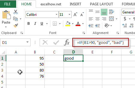
Note: the above excel formula will test a condition “b1>90”, if the condition is true, then “good” will return or “bad” will return.
Nested IF statements
The excel if function just only test one condition and if you want to deal with more than one condition and return different actions depending on the result of the tests, then you need to include several IF statements (functions) in one excel IF formula, these multiple IF statements are also called Excel Nested IF formula(Nested IFs).
For example:
=IF(A1>=80, "excellent", IF(A1>=60, "good", IF(A1>0, "bad", "no valid score")))
More reading: Excel Nexted IF Functions (Statements) Tutorial
Excel Logical operators
When you are writing an If statement, you may need to use any of the following excel logical operators:
| Operator | Meaning | Example | Description |
| = | Equal To | A1=B1 | Returns True if a value in cell A1 is equal to the values in cell B1; FALSE if they are not. |
| > | Greater Than | A1>B1 | Returns True if a value in cell A1 is greater than the values in cell B1; FALSE if they are not. |
| >= | Greater Than or Equal to | A1>=B1 | Returns True if a value in cell A1 is greater than or equal to the values in cell B1; FALSE if they are not. |
| < | Less Than | A1<B1 | Returns True if a value in cell A1 is less than the values in cell B1; FALSE if they are not. |
| <= | Less Than or Equal to | A1<=B1 | Returns True if a value in cell A1 is less than or equal to the values in cell B1; FALSE if they are not. |
| <> | Not Equal to | A1<>B1 | Returns True if a value in cell A1 is not equal to the values in cell B1; FALSE if they are not. |
Let’s see some examples for logical operators in Excel formula:
 =(A1>B1)
Output: TRUE

=(A1<B1)
Output: FALSE

=(A1>=B1)
Output: TRUE

=(A1<>8)
Output: FALSE

=(A1<>B1)
Output: TRUE

=(IF A1>3, “TRUE”, “FALSE”)
Output: TRUE
Frequently Asked Questions
Question1: I want to write an IF Formula based on the below test criteria in the Microsoft excel.
If the number in Cell B1 is greater than 30, then I want it to return A
If the number in cell B1 is between 20 and 30, then I want it to return B
If the number in Cell B1 is below 20, then I want it to return C
The below formula is what I currently write:
=IF(B1>30,"A",IF(B1<30,B1>20,"B","C"))
When I entered the above formula in the Cell C1, and it will return an Error.
Answer: You can use IF function in combination with AND function to reflect the above logic. So you can do it using the following formula:
=IF(B1>30,"A",IF(AND(B1>=20,B1<=30),"B","C"))
Or you can use another IF formula without AND function as follows:
=IF(B1>30,"A",IF(B1<20,"C","B"))
Question 2: I want to write a excel Formula for sales rep, If the sales are less than 10K, then the member will get no commission. If the sales are between 10 and 50K, then the member will get a 3% commission. If the sales are more than 50k, then the member will get 5% commission. Could you help me?
Answer: Based on the above description, we can use the following excel IF formula:
=IF(B1<10,0,IF(B1<50,B1*3%,B1*5%))
Question 3: I want to select students for the scholarship in school, and based on the student’s scores and attendance value, if the student scores more than 85 and has the attendance of more than 85%, then he/she will get the scholarship. Please help me how to write this formula based on my test criteria.
Answer: you can use the IF function with the AND function to check whether both of two conditions are met or not. If the test are met, then return “Yes”, otherwise returns “No”.
So you can use the following IF formula in Excel:
=IF(AND(B1>85, C1>85%),"Yes","No")
Question 4: I am trying to write an excel formula based on the following logic:
I want to enter a formula in Cell C1 that will Add B1, B2 and B3 or multiply B1 by 1, multiply B2 by 2, multiply B2 by 3, which action will be taken based on what you put in Cell D1.
Appreciated for any help. Thanks
Answer: Based on the above logic description, you need to use SUM function to count the sum of B1, B2 and B3. We can use the following IF formula:
=IF(D1="Add”,SUM(B1,B2,B3),IF(D1="Multiply",B1*B2*B3,"ERROR"))
Question 5: I am trying to write a formula in excel to check the employee number field and returns the relevant band of employee. I already have one IF formula, but I always return the first value of “A”. Could you help?
=IF(B1>=10,"A",IF(B1>=20,"B",IF(B1>=50,"C")))
Answer: when you write an IF nested formula, you need to start with the largest number first or start the smallest number first with less than or equal to operator.
1# start with the largest number first, we can write down the below formula:
=IF(B1>=50,"C",IF(B1>=20,"B",IF(B1>=10,"A")))
2# start with the smallest number first, you need to change the >= to <= , just see the below formula:
=IF(B1<=10,"A",IF(B1<=20,"B",IF(B1<=50,"C")))
Question 6: I want to write a Formula in excel to return “bad” if the cell B1 is either <100 or >500, otherwise, it should be returned the value of cell B1.
Answer: For the above logic test, we should use the OR function in the IF condition, so we can write down the below IF formula:
=IF(OR(B1>500,B1<100),"good",B1)
Question 7: I want to write a formula in excel using IF function to check if the cell B1 >10 and B1<20. If TRUE, returns “good”, If FALSE, returns “bad”
Answer: You can use IF function in combination with AND function to check the value of Cell B1, if cell B1 is greater than 10 and cell B1 is less than 20, then returns “good”, otherwise, it will return “bad”.
=IF(AND(B1>10,B1<20),"good","bad")
Question 8: I need to write a nested IF statement in excel 2013 to check the following logic:
If Cell B1 is less than 5, then multiply it by 5.
If Cell B1 is greater than or equal to 5 but less than 10, then multiply it by 10.
If cell B1 is greater than 10, then multiply it by 15.
Answer: This is a generic nested IF formula in excel, we can write the below nested IF statement to reflect the logic.
=IF(B1<5, B1*5, IF(B1<10, B1*10, B1*15))
Question 9: I want to write a formula to match the following logic in MS Excel 2013:
If A1*B1 <=10, then returns A
If A1*B1 >10 but A1*B1 <=20, then returns B
If A1*B1 >20 but A1*B1 <=30, then returns C
If A1*B1>30, then returns D
Answer: You can use IF function to build a Nested IF statement in combination with AND function to achieve it. Let’s write down the following IF formula:
=IF(A1*B1<=10,"A", IF(AND(A1*B1>10,A1*B1<=20),"B", IF(AND(A1*B1>20,a1*B1<=30,"C","D"))))
Question 10: I want to write an IF function to check if the value in cell B1 is blank or Text string or Numeric value, if the cell B1 is empty, then return “blank”, if the cell B1 is a text string, then return “Text”, if the value in cell B1 is a numeric value, then return “number”. Any help for this formula, thanks.
Answer: Based on the description, you need to use ISBLANK function to check if the value in cell b1 is blank or not. And need to use ISTEXT function to check if the value in cell B1 is a text string or not and need to use ISNUMBER function to check if the value in cell B1 is a number or not. So you can write a nested IF statements in combination with ISBLANK, ISTEXT and ISNUMBER functions in Excel as follows:
=IF(ISBLANK(B1),"blank", IF(ISTEXT(B1),"Text", IF(ISNUMBER(B1),"number")))
Question 11: I want to write a formula in excel to calculate the bonus for employees in company, if the employee salary is greater than or equal to $2000, then the bonus will be 10% of the salary , otherwise, the bonus will be 5% of the employee salary.
Answer: we need to check if the salary in Cell B1 (it’s the salary of the first employee) is greater than or equal to 2000. It the condition test is TRUE, then returns B1*10%, otherwise returns b1*5%. So we can write down the following IF formula in excel:
=IF(B1>=2000, B1*10%, B1*5%)
Question 12: In Microsoft Excel 2013, I want to create an IF function to check if any employee who have at least 10 years of experience and whose salary is greater than $5000, If TRUE, then the bonus will be 20% of salary.
Answer: you can use IF function in combination with AND function to check if the value in cell B1 is greater than or equal to 10 and the value in Cell C1 is greater than 5000. If both of two conditions are TRUE, then returns C1*20%, otherwise returns “No Bonus”.
Let’s write down the following IF statement as follows:
=IF(AND(B1>=10,C1>5000),C1*20%, "No Bonus")
Question 13: I want to create an IF formula in Excel 2013 to check the following text logic:
If B1<10, then multiply B1 by 1%, but the returned value is not less than 50.
If B1>10, then multiply B1 by 2%, but the returned value is not greater than 100.
Answer: To reflect the first test condition, you need to use MAX function to match the condition. To reflect the second test condition, you need to use MIN function to match that the returned value should not be greater than 100. So we can use the following excel IF formula:
=IF(B1<10, MAX(50,B1*1%), IF(B1>10, MIN(100,B1*5%)))
Question 14: I want to use IF function to check if B1 is greater than 10 and B2 is greater than 20 and B3 is less than 30, if TRUE, then returns “good”, otherwise, it should be returned “bad”. So How to create the IF formula based on the above test criteria to check three conditions at the same time.
Answer: you need to use AND function within the IF function in excel to create an IF formula as follows:
=IF(AND(B1>10,B2>20,B3<30),"good","bad")
Question 15: I have an IF formula that might cause a division by zero error, I don’t know how to avoid this kind of errors in Excel formula.
Answer: You can use ISERROR function to catch this kind of errors then use the IF function to check the returned values from ISERROR function to avoid an error. So we can write an IF function in combination with ISERROR function in excel. For example, we can use the following IF formula:
=IF(ISERROR(B1/C1),0, B1/C1)
The ISERROR function will return TRUE when trying to divide B1 by 0.
Question 16: I need to create a formula in Excel 2013 to reflect the following logic:
If B1=Excel, then return E
If B1=word, then return W
If B1=access, then return A
Answer: You can use IF function to create a nested IF statements as follows:
=IF(B1="Excel","E",IF(B1="word","W",IF(B1="access","A")))
Question 17: I have a worksheet that containing cells that are formatted as date format. I want to write an IF formula to check the first value in Cell (month part). So I am trying to create the following IF formula:
=IF(LEFT(B1,1)=8, "August","Null")
The returned results are always “Null”.
Answer: As the dates are not recognized as string, so you cannot use the LEFT function to exact the first value in the dates. At this moment, you need to use Month function to convert the date to its month number in Excel. So we can write down the below IF formula in combination with Month function:
=IF(MONTH(B1)=8, "August","Null")
Question18: I am trying to create an IF formula to check if the time value in cells are greater than 10.00h for the following date format: 08/11/2018 09:43.50. Appreciative of any help.
Answer: In excel, you can use HOUR, MINUTE, SECOND functions to compare the date or time value. so if you want to compare the value in Cell B1 if it is greater than 10h, then you can use HOUR function within IF function, just like this: HOUR(B1)>10, so we can write down the below formula:
=IF(HOUR(B1)>10, "greater","less")
Question 19: I want to create an IF function and need to combine with another RAND function. The formula just works find for the first IF_VALUE_TRUE statement, but the formula works not good for IF_VALUE_FALSE statement. Here is the IF formula I have got:
=IF(ISBLANK(B1),"","=rand()")
In the above IF function, it will return empty string when the value in cell B1 is blank. Otherwise, it should add a random function, the problem is that the cell doesn’t run the RAND function. So how can I fix it? Thanks
Answer: when you write an IF formula, if you want to enclose others function, you need not to add quotes around the RAND () function, so just remove the quotes and equal sign in your IF function. Just like the below IF formula:
=IF(ISBLANK(B1),"",RAND())
Question 20: I am trying to write an IF formula in Excel 2013 to reflect the following logic:
If B1 is greater than or equal to 50 and C1 is 0
OR
If B1 is greater than or equal to 30 and C1 is greater than or equal to 1
OR
If B1 is greater than or equal to 20 and C1 is 2
Then take the following action: D2/E2
Otherwise, return FALSE
I have wrote the following IF formula, but it doesn’t work at all.
=IF(AND(B1>=50,C1>=0),OR(AND(B1>=30,C1>=1)),OR(AND(B1>=20,C1>=2)),D2/E2,"FALSE")
Answer: you need to nest your different AND function within an OR function in the IF formula. So you can try the below IF formula:
=IF(OR(AND(B1>=50,C1>=0),AND(B1>=30,C1>=1),AND(B1>=20,C1>=2)), D2/E2,"FALSE")
Question 21: I want to create an IF function in combination with MID function in excel 2013. it need to check if the value in one specified cell is TRUE, then return the first six characters from another cell. Otherwise return empty value.
Answer: you just need to add MID function within IF function in excel, and do not add any quotes around MID function. So you can use the following IF formula to achieve your request:
=IF(B1=TRUE, MID(C1,1,5), "")
Question 22: I have a excel worksheet as below:
A B
——
20 O
30 V
10 T
50 T
I want to create an IF formula to reflect the following logic:
IF cell A1 is less than or equal to 30 and Cell B1 is equal to “O” or “V”, if TRUE, then returns 300, otherwise returns 400.
IF Cell A1 is greater than 30 and Cell B1 is equal to “O” or “V”, then returns 500, otherwise returns 600.
I have wrote the below tow IF formulas for the above two conditions as follows:
=IF(AND(A1<=30,OR(B1="O",B1="V")),300,400)
=IF(AND(A1>30,OR(B1="O",B1="V")),500,600)
I am able to check the above two IF formula and the returned results is OK… But I am not able to combine the above two IF formula into a single IF formula. So anybody can help? Many thanks
Answer: Based on the above logic, you can use the below IF formula to combine with above two IF formulas:
=IF(A1<=30,IF(OR(B1="O",B1="V"),300,400),IF(OR(B1="O",B1="V"),500,600))
Question 23: I am trying to write an IF function to prevent zero and negative values in cells. What I would like is that if the value in cell B1 is less than or equal to 0, then it should be returned “Null” otherwise, it should return the calculation of Cells value, like as:B2*(C2-D2)*E2.
The below IF formula is what I have:
=IF(B1<=0,"Null","B2*(C2-D2)*E2")
When I run the formula above, it only returns my calculation string and do not take the actual calculation.
Answer: In excel, the double quotes make any values in between be recognized as Text string. So if you want to take calculation for your IF formula, just remove the double quotes. Let’s see the modified IF formula as follows:
=IF(B1<=0,"Null",B2*(C2-D2)*E2)
Question 24: I want to create an new IF function to check if the value in cells is Saturday or Sunday, If TRUE, returns “yes”, otherwise, returns “No”. And I am using the following IF formula, but I get an error, so what’s wrong for this formula?
=IF((OR($B1="Saturday","$B1="Sunday"),"yes","no"))
Answer: you need to use the WEEKDAY function within IF function to handle the dates if they are in date format, like as: 11/8/2018.
So you can use the below IF function to achieve your logic:
=IF(WEEKDAY($B$1,2)>5,"yes","no")
You can also use TEXT function within the IF function to achieve the same results, just like the below IF formula:
=IF(LEFT(TEXT($B$1,"ddd"))="S","yes","no")
Question 25: I want to write an IF function in excel to check if the first character in one Cell is equal to 5, then the returned value should be the five rightmost characters of that cell, otherwise, the returned value should be the four rightmost characters. I wrote one IF formula as follows, but it doesn’t work.
=IF(LEFT(B1,1)=5, RIGHT(B1,5),RIGHT(B1,4))
In the above IF function, it always return the rightmost four characters even though the first character in Cell B1 starts with “S”. Please help me to fix it.
Answer: you should know the returned value of the LEFT function firstly in excel. As the LEFT function will return a Text value, so you also need to provide a string for comparison, so adding quotes to enclose it. Just like the below IF function:
=IF(LEFT(B1,1)="5", RIGHT(B1,5),RIGHT(B1,4))
There is another way to achieve the same results, you can use NUMBERVALUE function to convert the result of LEFT function to a numeric value, like the below IF function:
=IF(NUMBERVALUE(LEFT(B1,1))=5,RIGHT(B1,5),RIGHT(B1,4))
Question 26: I have 2 columns contain date and time or just only contain time. And I want to check if the times of column A is greater than the times of column B. the key issue may be that column A has the date and time. I wrote the following IF formula to run it in Cell C1, but it returned the inaccurate results.
=IF(A1>B1,"yes","no")
Any help would be appreciated… Many thanks!
Answer: the date part of the value in column A is the integer, while the time is the decimal. You can use the following IF formula:
=IF(A1-INT(A1)>B2),"yes","no")
Question 27: The below are the results that I expected, and I want cell B1 to B4 can detect the string from A1 to A4 automatically and return the same string value plus the severity level when the test match. For example, If A1 is equal to “critical”, then it should be returned “critical severity 1” in the cell B1. Etc.
And I am using the following IF formula, but it does not work at all. Please help to fix it. Thanks
=IF(A1="Critical","Critical Severity 1",""),IF(A1="High","High Severity 2",""),IF(A1="Medium","Medium Severity 3",""),IF(A1="Low","Low Severity 4","")
| A | B |
| critical | critical severity 1 |
| high | high severity 2 |
| medium | Medium severity 3 |
| low | low severity 4 |
Answer: you can try to run the following IF formula in excel:
=IF(A1="critical","critical Severity 1",IF(A1="high","high Severity 2",IF(A1="medium","medium Severity 3",IF(A1="low","low Severity 4",""))))
Question 28: I am working on an excel file and want to create a new IF formula to reflect the following logic:
If the value in Cell A1 is equal to the value in Cell A2, then check if the minus of B1 and B2 is equal to a special value, and if the condition is TRUE, returns “yes”, otherwise, returns “no”. Here is the IF formula I have:
=if(A1=A2,B1-B2=5 or B1-B2=-5 or B1-B2=20 or B1-B2=-20, "yes", "no")
Any help is appreciated…Thanks
Answer: you need to use OR function with IF function to create a nested IF statement to achieve your request. So you can try the following Excel IF formula in your excel file.
=IF(A1=A2,IF(OR(B1-B2=5,B1-B2=-5,B1-B2=20,B1-B2=-20),"yes","no"),"no")
Question 29: I want to create an IF formula to check the range of cells in excel. I have scores of different subject for a student, and want to check if any one of scores is less than 60, If TRUE, then return “BAD”. Can this logic be done with the IF statements in excel 2013?
Answer: you can use COUNTIF function within IF function to create a generic IF formula as follows:
=IF(COUNTIF(B:B,"<60")>0,"BAD","Good")
Question 30: I am trying to create a new IF statement so that when the formula is looking at Row A and Row B, the returned values should be shown in the Row C. the following logic need to be checked:
IF the value in the Row A is equal to “NA” And the value in the Row B is equal to “NA”, then return “NA” value in Row C.
IF the value in the Row A is equal to “NA”, and the value in the Row B is equal to “denied”, then return “denied” value in Row C.
IF the value in the Row A is equal to “allowed” and the value in the Row B is equal to “NA”, then return “allowed” value in Row C.
Here is my formula:
=IF(AND(A1 = "NA", B1 = "NA"),"NA",IF(OR(A1="denied",B1 ="denied"),"denied", "NA"))
I don’t know how to include “allowed” in the IF formula above, anyone can help this, many thanks.
Answer: This is a typical nested if statement, you can use OR function within IF function in excel. We can write down this nested IF formula as follows:
=IF(OR(A1="denied", B1="denied"), "denied", IF(OR(A1="allowed", B1="allowed"), "allowed", "NA"))
- Excel AND function
The Excel AND function returns TRUE if all of arguments are TRUE, and it returns FALSE if any of arguments are FALSE.The syntax of the AND function is as below:= AND (condition1,[condition2],…) … - Excel ISBLANK function
The Excel ISBLANK function returns TRUE if the value is blank or null.The syntax of the ISBLANK function is as below:= ISBLANK (value)… - Excel COUNTIF function
The Excel COUNTIF function will count the number of cells in a range that meet a given criteria.= COUNTIF (range, criteria) … - Excel ISERROR function
The Excel ISERROR function returns TRUE if the value is any error value except #N/A. The ISERROR function is a build-in function in Microsoft Excel and it is categorized as an Information Function. The syntax of the ISERROR function is as below: = ISERROR (value) … - Excel LEFT function
The Excel LEFT function returns a substring (a specified number of the characters) from a text string, starting from the leftmost character.The syntax of the LEFT function is as below:= LEFT(text,[num_chars])… - Excel MID function
The Excel MID function returns a substring from a text string at the position that you specify. The MID function is a build-in function in Microsoft Excel and it is categorized as a Text Function. The syntax of the MID function is as below: = MID (text, start_num, num_chars) … - Excel TEXT function
The Excel TEXT function converts a numeric value into text string with a specified format. The syntax of the TEXT function is as below:= TEXT (value, Format code)… - Excel RIGHT function
The Excel RIGHT function returns a substring (a specified number of the characters) from a text string, starting from the rightmost character…
More Excel IF Formula Examples
- Excel nested if function
The nested IF function is formed by multiple if statements within one Excel if function. This excel nested if statement makes it possible for a single formula to take multiple actions… - Excel IF formula with Equal to logical operators
The “Equal to” logical operator can be used to compare the below data types, such as: text string, numbers, dates, Booleans. This section will guide you how to use equal to logical operator in excel IF formula with text string value and dates value… - Excel IF formula with greater than logical operators
How to use if function with greater than, greater than or equal to, less than and less than or equal to logical operators in excel. Let’s see the below generic if formula with greater than operator: =IF(A1>10,”excelhow.net”,”google”) … - Excel IF formula with AND logical function
You can use the IF function combining with AND function to construct a condition statement. If the test is FALSE, then take another action. The syntax of AND function in excel is as follow: =AND(condition1,[condition2],…)… - Excel IF function with OR logical function
If you want to check if one of several conditions is met in your excel workbook, if the test is TRUE, then you can take certain action. You can use the IF function combining with OR function to construct a condition statement… - Excel IF function with “NOT” logical function
If you want to check several test conditions in an excel formula, then take different actions. You can use NOT function in combination with the AND or OR logical function in excel IF function… - Excel IF formula with AND & OR logical functions
If you want to test the result of cells based on several sets of multiple test conditions, you can use the IF function with the AND and OR functions at a time… - Excel IF Function With Numbers
If you want to check if a cell values is between two values or checking for the range of numbers or multiple values in cells, at this time, we need to use AND or OR logical function in combination with the logical operator and IF function… - Excel IF function with text values
If you want to write an IF formula for text values in combining with the below two logical operators in excel, such as: “equal to” or “not equal to”… - Excel IF function with Dates
If you have a list of dates and then want to compare to these dates with a specified date to check if those dates is greater than or less than that specified date. … - Excel IF function check if the cell is blank or not-blank
If you want to check the value in one cell if it is blank or empty cell, then you can use IF function in combination with ISBLANK function or logical operator (equal to) in excel… -
Excel nested if statements with ranges
Many people usually asked that how to write an excel nested if statements based on multiple ranges of cells to return different values in a cell? How to nested if statement using date ranges? How to use nested if statement between different values in excel 2013 or 2016… - Count Cells That Contain Specific Text
This post will discuss that how to count the number of cells that contain specific text or certain text in a specified cells of range in Excel. How to get the total number of cells that contain certain text.…… - Sum Values by Group
Assuming that you have a table that contain the product name and its sales result. And you have group by those values based on the product name, then you want to sum values based one each product name. You can create a new Excel formula based on the IF function and SUMIF function.… - Get nth Largest Value with Duplicates
If you want to get the largest unique value in a data set with duplicates, you can create a new excel array formula based on the MAX function and the IF function..… - Find the Largest Value Based on Multiple Criteria
Assuming that you have a list of data that you want to find the largest value based on the product “excel” and the sales region “east”. You can create a new excel formula based on the SUMPRODUCT function and the LARGE function..…… - Create a Five Star Rating System
How do I change the five points system to five star rating in excel. How to use the conditional formatting function to create a five star rating system in excel….. - Rank values in a column based a specific value in another column
Assuming that you have a list of data contains two columns and the first column is product list and another is Sales number. You want to rank the sales number of a specified product name. You can try to write a complex formula based on the IF function and the COUNTIFS function to achieve the result..… - Comparing Columns Using Conditional Formatting Icon Sets
how to compare the adjacent cells in the different columns using Conditional Formatting Icon Sets in Excel. How to compare Columns or rows using Conditional Formatting Icon Sets to show increase or decrease status in your current worksheet..… - Show Only Positive Values
You can create a formula based on the IF function, and the SUM function to sum all values in the range A1:C5 and just show only positive values… - Count Unique Values Using Pivot Table
You can insert a 3rd or helper column with a formula to check if the value is unique in the selected range of cells, and the create pivot table based on the 1st and 3rd column to count unique values..… - Compare Dates
Assuming that you have a list of data that contain date values in Excel, you can use the IF function to create a formula to achieve it. If the date is greater that the given date value, then return True. Otherwise, it returns False…. - Excel Vlookup Return True or False
you can use the VLOOKUP function to look for a value in a column in a table and then returns TRUE from a given column in that table if it finds something. If it doesn’t, it returns FALSE … - VLOOKUP Return Multiple Values Horizontally
You can create a complex array formula based on the INDEX function, the SMALL function, the IF function, the ROW function and the COLUMN function to vlookup a value and then return multiple corresponding values horizontally in Excel.… - Copy and Paste Only Non-blank Cells
If you want only copy non-blank cells in a range in Excel, you need to select the non-blank cells firstly, then press Ctrl +C keys to copy the selected cells. So how to only select all non-blank cells in the selected range in your worksheet..… - Changing Negative Number to Zero in Excel
If you want to change all negative numbers to zero value from a cell in Excel, you can use a formula based on the MAX function or IF function.… - Count Dates in Given Year/Month/Day in Excel
You can create a formula based on the SUMPRODUCT function and the YEAR function to count dates by a give year…. - Generate All Possible Combinations of Two Lists
You can use a formula based on the IF function, the ROW function, the COUNTA function, The INDEX function and the MOD function to get a list of all possible combinations from those two list…. - Find Missing Numbers in a Sequence in Excel
You can use an excel array formula based on the SMALL function, the IF function, the ISNA function, the MATCH function, and the ROW function to find missing numbers in a sequence…
What is IF Function in Excel?
IF function in Excel evaluates whether a given condition is met and returns a value depending on whether the result is “true” or “false”. It is a conditional function of Excel, which returns the result based on the fulfillment or non-fulfillment of the given criteria.
For example, the IF formula in Excel can be applied as follows:
“=IF(condition A,“value B”,“value C”)”
The IF excel function returns “value B” if condition A is met and returns “value C” if condition A is not met.
It is often used to make logical interpretations which help in decision-making.
Table of contents
- What is IF Function in Excel?
- Syntax of the IF Excel Function
- How to Use IF Function in Excel?
- Example #1
- Example #2
- Example #3
- Example #4
- Example #5
- Guidelines for the Multiple IF Statements
- Frequently Asked Question
- IF Excel Function Video
- Recommended Articles
Syntax of the IF Excel Function
The syntax of the IF function is shown in the following image:

The IF excel function accepts the following arguments:
- Logical_test: It refers to the condition to be evaluated. The condition can be a value or a logical expression.
- Value_if_true: It is the value returned as a result when the condition is “true”.
- Value_if_false: It is the value returned as a result when the condition is “false”.
In the formula, the “logical_test” is a required argument, whereas the “value_if_true” and “value_if_false” are optional arguments.
The IF formula uses logical operators to evaluate the values in a range of cells. The following table shows the different logical operatorsLogical operators in excel are also known as the comparison operators and they are used to compare two or more values, the return output given by these operators are either true or false, we get true value when the conditions match the criteria and false as a result when the conditions do not match the criteria.read more and their meaning.
| Operator | Meaning |
|---|---|
| = | Equal to |
| > | Greater than |
| >= | Greater than or equal to |
| < | Less than |
| <= | Less than or equal to |
| <> | Not equal to |
How to Use IF Function in Excel?
Let us understand the working of the IF function with the help of the following examples in Excel.
You can download this IF Function Excel Template here – IF Function Excel Template
Example #1
If there is no oxygen on a planet, life is impossible. If oxygen is available on a planet, then life is possible. The following table shows a list of planets in column A and the information on the availability of oxygen in column B. We have to find the planets where life is possible, based on the condition of oxygen availability.

Let us apply the IF formula to cell C2 to find out whether life is possible on the planets listed in the table.
The IF formula is stated as follows:
“=IF(B2=“Yes”, “Life is Possible”, “Life is Not Possible”)
The succeeding image shows the IF formula applied to cell C2.

The subsequent image shows how the IF formula is applied to the range of cells C2:C5.

Drag the cells to view the output of all the planets.

The output in the below worksheet shows life is possible on the planet Earth.
Flow Chart of Generic IF Excel Function

The IF Function Flow Chart for Mars (Example #1)

The flow of IF function flowchart for Jupiter and Venus is the same as the IF function flowchart for Mars (Example #1).
The IF Function Flow Chart for Earth

Hence, the IF excel function allows making logical comparisons between values. The modus operandi of the IF function is stated as: If something is true, then do something; otherwise, do something else.
Example #2
The following table shows a list of years. We want to find out if the given year is a leap year or not.
A leap year has 366 days; the extra day is the 29th of February. The criteria for a leap year are stated as follows:
- The year will be exactly divisible by 4 and not exactly be divisible by 100 or
- The year will be exactly divisible by 400.

In this example, we will use the IF function along with the AND, OR, and MOD functions to find the leap years.
We use the MOD function to find a remainder after a dividend is divided by a divisor.
The AND functionThe AND function in Excel is classified as a logical function; it returns TRUE if the specified conditions are met, otherwise it returns FALSE.read more evaluates both the conditions of the leap years for the value “true”. The OR functionThe OR function in Excel is used to test various conditions, allowing you to compare two values or statements in Excel. If at least one of the arguments or conditions evaluates to TRUE, it will return TRUE. Similarly, if all of the arguments or conditions are FALSE, it will return FASLE.read more evaluates either of the condition for the value “true”.
We will apply the MOD function to the conditions as follows:
If MOD(year,4)=0 and MOD(year,100)<>(is not equal to) 0, then the year is a leap year.
or
If MOD(year,400)=0, then the year is a leap year; otherwise, the year is not a leap year.
The IF formula is stated as follows:
“=IF(OR(AND((MOD(year,4)=0),(MOD(year,100)<>0)),(MOD(year,400)=0)),“Leap Year”, “Not A Leap Year”)”
The argument “year” refers to a reference value.
The following images show the output of the IF formula applied in the range of cells.


The following image shows how the IF formula is applied to the range of cells B2:B18.

The succeeding table shows the years 1960, 2028, and 2148 as leap years and the remaining as non-leap years.

The result of the IF excel formula is displayed for the range of cells B2:B18 in the following image.

Example #3
The succeeding table shows a list of drivers and the directions they undertook to reach the destination. It is preceded by an image of the road intersection explaining the turns taken by the drivers and their destinations. The right turn leads to town B, and the left turn leads to town C. Identify the driver’s destination to town B and town C.
Road Intersection Image


Let us apply the IF excel function to find the destination. Here, the condition is mentioned as follows:
- If the driver turns right, he/she reaches town B.
- If the driver turns left, he/she reaches town C.
We use the following IF formula to find the destination:
“=IF(B2=“Left”, “Town C”, “Town B”)”
The succeeding image shows the output of the IF formula applied to cell C2.

Drag the cells to use the formula in the range C2:C11. Finally, we get the destinations of each driver for their turning movements.
The below image displays the IF formula applied to the range.

The output of the IF formula and the destinations are displayed in the succeeding image.

The result shows that six drivers reached town C, and the remaining four have reached town B.
Example #4
The following table shows a list of items and their inventory levels. We want to check if the specific item is available in the inventory or not using the IF function.

Let us list the name of items in column A and the number of items in column B. The list of data to be validated for the entire items list is shown in the cell E2 of the below image.

We use the Excel IF along with the VLOOKUP functionThe VLOOKUP excel function searches for a particular value and returns a corresponding match based on a unique identifier. A unique identifier is uniquely associated with all the records of the database. For instance, employee ID, student roll number, customer contact number, seller email address, etc., are unique identifiers.
read more to check the availability of the items in the inventory.
The VLOOKUP function looks up the values referring to the number of items, and the IF function will check whether the item number is greater than zero or not.
We will apply the following IF formula in the F2 cell:
“=IF(VLOOKUP(E2,A2:B11,2,0)=0, “Item Not Available”,“Item Available”)”
If the lookup value of an item is equal to 0, then the item is not available; else, the item is available.
The succeeding image shows the result of the IF formula in the cell F2.

Select “bat” in the E2 item cell to know whether the item is available or not in the inventory (as shown in the following image).

Example #5
The following table shows the list of students and their marks. The grade criteria are provided based on the marks obtained by the students. We want to find the grade of each student in the list.

We apply the Nested IF in Excel since we have multiple criteria to find and decide each student’s grade.
The Nesting of IF function uses the IF function inside another IF formula when multiple conditions are to be fulfilled.
The syntax of Nesting of IF function is stated as follows:
“=IF( condition1, value_if_true1, IF( condition2, value_if_true2, value_if_false2 ))”
The succeeding table represents the range of scores and the grades, respectively.

Let us apply the multiple IF conditions with AND function in the below-nested formula to find out the grade of the students:
“=IF((B2>=95),“A”,IF(AND(B2>=85,B2<=94),“B”,IF(AND(B2>=75,B2<=84),“C”,IF(AND(B2>=61,B2<=74),“D”,“F”))))”
The IF function checks the logical condition as shown in the formula below:
“=IF(logical_test, [value_if_true],[value_if_false])”
We will split the above-mentioned nested formula and check the IF statements as shown below:
First Logical Test: B2>=95
If the formula returns,
- Value_if_true, execute: “A” (Grade A) else(comma) enter value_if_false
- Value_if_false, then the formula finds another IF condition and enter IF condition
Second Logical Test: B2>=85(logical expression 1) and B2<=94(logical expression 2)
(We use AND function to check the multiple logical expressions as the two given conditions are to be evaluated for “true.”)
If the formula returns,
- Value_if_true, execute: “B” (Grade B) else(comma) enter value_if_false
- Value_if_false, then the formula finds another IF condition and enter IF condition
Third Logical Test: B2>=75(logical expression 1) and B2<=84(logical expression 2)
(We use AND function to check the multiple logical expressions as the two given conditions are to be evaluated for “true.”)
If the formula returns,
- Value_if_true, execute: “C” (Grade C) else(comma) enter value_if_false
- value_if_false, then the formula finds another IF condition and enter IF condition
Fourth Logical Test: B2>=61(logical expression 1) and B2<=74(logical expression 2)
(We use AND function to check the multiple logical expressions as the two given conditions are to be evaluated for “true.”)
If the formula returns,
- Value_if_true, execute: “D” (Grade D) else(comma) enter value_if_false
- Value_if_false, execute: “F” (Grade F)
- Finally, close the parenthesis.
The below image displays the output of the IF formula applied to the range.

The succeeding image shows the IF nested formula applied to the range.

The grades of the students are listed in the following table.

Guidelines for the Multiple IF Statements
The guidelines for the multiple IF statements are listed as follows:
- Use nested IF function to a limited extent as multiple IF statements require a great deal of thought to be accurate.
- Multiple IF statementsIn Excel, multiple IF conditions are IF statements that are contained within another IF statement. They are used to test multiple conditions at the same time and return distinct values. Additional IF statements can be included in the ‘value if true’ and ‘value if false’ arguments of a standard IF formula.read more require multiple parentheses (), which is often difficult to manage. Excel provides a way to check the color of each opening and closing parenthesis to avoid this situation. The last closing parenthesis color will always be black, denoting the end of the formula statement.
- Whenever we pass a string value for the arguments “value_if_true” and “value_if_false” or test a reference against a string value, enclose the string value in double quotes. Passing a string value without quotes will result in “#NAME?” error.
Frequently Asked Question
1. What is the IF function in Excel?
The Excel IF function is a logical function that checks the given criteria and returns one value for a “true” and another value for a “false” result.
The syntax of the IF function is stated as follows:
“=IF(logical_test, [value_if_true], [value_if_false])”
The arguments are as follows:
1. Logical_test – It refers to a value or condition that is tested.
2. Value_if_true – It is the value returned when the condition logical_test is “true.”
3. Value_if_false – It is the value returned when the condition logical_test is “false.”
The “logical_test” is a required argument, whereas the “value_if_true” and “value_if_false” are optional arguments.
2. How to use the IF Excel function with multiple conditions?
The IF Excel statement for multiple conditions is created by using multiple IF functions in a single formula.
The syntax of IF function with multiple conditions is stated as follows:
“=IF (condition 1_“true”, do something, IF (condition 2_“true”, do something, IF (condition 3_ “true”, do something, else do something)))”
3. How to use the function IFERROR in Excel?
IF Excel Function Video
Recommended Articles
This has been a guide to the IF function in Excel. Here we discuss how to use the IF function along with examples and downloadable templates. You may also look at these useful functions –
- What is the Logical Test in Excel?A logical test in Excel results in an analytical output, either true or false. The equals to operator, “=,” is the most commonly used logical test.read more
- “Not Equal to” in Excel“Not Equal to” argument in excel is inserted with the expression <>. The two brackets posing away from each other command excel of the “Not Equal to” argument, and the user then makes excel checks if two values are not equal to each other.read more
- Data Validation ExcelThe data validation in excel helps control the kind of input entered by a user in the worksheet.read more
The logical IF statement in Excel is used for the recording of certain conditions. It compares the number and / or text, function, etc. of the formula when the values correspond to the set parameters, and then there is one record, when do not respond — another.
Logic functions — it is a very simple and effective tool that is often used in practice. Let us consider it in details by examples.
The syntax of the function «IF» with one condition
The operation syntax in Excel is the structure of the functions necessary for its operation data.
=IF(boolean;value_if_TRUE;value_if_FALSE)
Let us consider the function syntax:
- Boolean – what the operator checks (text or numeric data cell).
- Value_if_TRUE – what will appear in the cell when the text or numbers correspond to a predetermined condition (true).
- Value_if_FALSE – what appears in the box when the text or the number does not meet the predetermined condition (false).
Example:

Logical IF functions.
The operator checks the A1 cell and compares it to 20. This is a «Boolean». When the contents of the column is more than 20, there is a true legend «greater 20». In the other case it’s «less or equal 20».
Attention! The words in the formula need to be quoted. For Excel to understand that you want to display text values.
Here is one more example. To gain admission to the exam, a group of students must successfully pass a test. The results are listed in a table with columns: a list of students, a credit, an exam.

The statement IF should check not the digital data type but the text. Therefore, we prescribed in the formula В2= «done» We take the quotes for the program to recognize the text correctly.
The function IF in Excel with multiple conditions
Usually one condition for the logic function is not enough. If you need to consider several options for decision-making, spread operators’ IF into each other. Thus, we get several functions IF in Excel.
The syntax is as follows:
Here the operator checks the two parameters. If the first condition is true, the formula returns the first argument is the truth. False — the operator checks the second condition.
Examples of a few conditions of the function IF in Excel:

It’s a table for the analysis of the progress. The student received 5 points:
- А – excellent;
- В – above average or superior work;
- C – satisfactory;
- D – a passing grade;
- E – completely unsatisfactory.
IF statement checks two conditions: the equality of value in the cells.

In this example, we have added a third condition, which implies the presence of another report card and «twos». The principle of the operator is the same.
Enhanced functionality with the help of the operators «AND» and «OR»
When you need to check out a few of the true conditions you use the function И. The point is: IF A = 1 AND A = 2 THEN meaning в ELSE meaning с.
OR function checks the condition 1 or condition 2. As soon as at least one condition is true, the result is true. The point is: IF A = 1 OR A = 2 THEN value B ELSE value C.
Functions AND & OR can check up to 30 conditions.
An example of using the operator AND:

It’s the example of using the logical operator OR.

How to compare data in two tables
Users often need to compare the two spreadsheets in an Excel to match. Examples of the «life»: compare the prices of goods in different bringing, to compare balances (accounting reports) in a few months, the progress of pupils (students) of different classes, in different quarters, etc.
To compare the two tables in Excel, you can use the COUNTIFS statement. Consider the order of application functions.
For example, consider the two tables with the specifications of various food processors. We planned allocation of color differences. This problem in Excel solves the conditional formatting.
Baseline data (tables, which will work with):

Select the first table. Conditional Formatting — create a rule — use a formula to determine the formatted cells:

In the formula bar write: = COUNTIFS (comparable range; first cell of first table)=0. Comparing range is in the second table.
To drive the formula into the range, just select it first cell and the last. «= 0» means the search for the exact command (not approximate) values.
Choose the format and establish what changes in the cell formula in compliance. It’s better to do a color fill.
Select the second table. Conditional Formatting — create a rule — use the formula. Use the same operator (COUNTIFS). For the second table formula:
Download all examples in Excel

Now it is easy to compare the characteristics of the data in the table.