
Sometimes, Excel seems too good to be true. All I have to do is enter a formula, and pretty much anything I’d ever need to do manually can be done automatically.
Need to merge two sheets with similar data? Excel can do it.
Need to do simple math? Excel can do it.
Need to combine information in multiple cells? Excel can do it.
In this post, I’ll go over the best tips, tricks, and shortcuts you can use right now to take your Excel game to the next level. No advanced Excel knowledge required.
![Download 10 Excel Templates for Marketers [Free Kit]](https://no-cache.hubspot.com/cta/default/53/9ff7a4fe-5293-496c-acca-566bc6e73f42.png)
-
What is Excel?
-
Excel Basics
-
How to Use Excel
-
Excel Tips
-
Excel Keyboard Shortcuts
What is Excel?
Microsoft Excel is powerful data visualization and analysis software, which uses spreadsheets to store, organize, and track data sets with formulas and functions. Excel is used by marketers, accountants, data analysts, and other professionals. It’s part of the Microsoft Office suite of products. Alternatives include Google Sheets and Numbers.
Find more Excel alternatives here.
What is Excel used for?
Excel is used to store, analyze, and report on large amounts of data. It is often used by accounting teams for financial analysis, but can be used by any professional to manage long and unwieldy datasets. Examples of Excel applications include balance sheets, budgets, or editorial calendars.
Excel is primarily used for creating financial documents because of its strong computational powers. You’ll often find the software in accounting offices and teams because it allows accountants to automatically see sums, averages, and totals. With Excel, they can easily make sense of their business’ data.
While Excel is primarily known as an accounting tool, professionals in any field can use its features and formulas — especially marketers — because it can be used for tracking any type of data. It removes the need to spend hours and hours counting cells or copying and pasting performance numbers. Excel typically has a shortcut or quick fix that speeds up the process.
You can also download Excel templates below for all of your marketing needs.
After you download the templates, it’s time to start using the software. Let’s cover the basics first.
Excel Basics
If you’re just starting out with Excel, there are a few basic commands that we suggest you become familiar with. These are things like:
- Creating a new spreadsheet from scratch.
- Executing basic computations like adding, subtracting, multiplying, and dividing.
- Writing and formatting column text and titles.
- Using Excel’s auto-fill features.
- Adding or deleting single columns, rows, and spreadsheets. (Below, we’ll get into how to add things like multiple columns and rows.)
- Keeping column and row titles visible as you scroll past them in a spreadsheet, so that you know what data you’re filling as you move further down the document.
- Sorting your data in alphabetical order.
Let’s explore a few of these more in-depth.
For instance, why does auto-fill matter?
If you have any basic Excel knowledge, it’s likely you already know this quick trick. But to cover our bases, allow me to show you the glory of autofill. This lets you quickly fill adjacent cells with several types of data, including values, series, and formulas.
There are multiple ways to deploy this feature, but the fill handle is among the easiest. Select the cells you want to be the source, locate the fill handle in the lower-right corner of the cell, and either drag the fill handle to cover cells you want to fill or just double click:
 Similarly, sorting is an important feature you’ll want to know when organizing your data in Excel.
Sometimes you may have a list of data that has no organization whatsoever. Maybe you exported a list of your marketing contacts or blog posts. Whatever the case may be, Excel’s sort feature will help you alphabetize any list.
Click on the data in the column you want to sort. Then click on the «Data» tab in your toolbar and look for the «Sort» option on the left. If the «A» is on top of the «Z,» you can just click on that button once. If the «Z» is on top of the «A,» click on the button twice. When the «A» is on top of the «Z,» that means your list will be sorted in alphabetical order. However, when the «Z» is on top of the «A,» that means your list will be sorted in reverse alphabetical order.
Let’s explore more of the basics of Excel (along with advanced features) next.
To use Excel, you only need to input the data into the rows and columns. And then you’ll use formulas and functions to turn that data into insights.
We’re going to go over the best formulas and functions you need to know. But first, let’s take a look at the types of documents you can create using the software. That way, you have an overarching understanding of how you can use Excel in your day-to-day.
Documents You Can Create in Excel
Not sure how you can actually use Excel in your team? Here is a list of documents you can create:
- Income Statements: You can use an Excel spreadsheet to track a company’s sales activity and financial health.
- Balance Sheets: Balance sheets are among the most common types of documents you can create with Excel. It allows you to get a holistic view of a company’s financial standing.
- Calendar: You can easily create a spreadsheet monthly calendar to track events or other date-sensitive information.
Here are some documents you can create specifically for marketers.
- Marketing Budgets: Excel is a strong budget-keeping tool. You can create and track marketing budgets, as well as spend, using Excel. If you don’t want to create a document from scratch, download our marketing budget templates for free.
- Marketing Reports: If you don’t use a marketing tool such as Marketing Hub, you might find yourself in need of a dashboard with all of your reports. Excel is an excellent tool to create marketing reports. Download free Excel marketing reporting templates here.
- Editorial Calendars: You can create editorial calendars in Excel. The tab format makes it extremely easy to track your content creation efforts for custom time ranges. Download a free editorial content calendar template here.
- Traffic and Leads Calculator: Because of its strong computational powers, Excel is an excellent tool to create all sorts of calculators — including one for tracking leads and traffic. Click here to download a free premade lead goal calculator.
This is only a small sampling of the types of marketing and business documents you can create in Excel. We’ve created an extensive list of Excel templates you can use right now for marketing, invoicing, project management, budgeting, and more.
In the spirit of working more efficiently and avoiding tedious, manual work, here are a few Excel formulas and functions you’ll need to know.
Excel Formulas
It’s easy to get overwhelmed by the wide range of Excel formulas that you can use to make sense out of your data. If you’re just getting started using Excel, you can rely on the following formulas to carry out some complex functions — without adding to the complexity of your learning path.
- Equal sign: Before creating any formula, you’ll need to write an equal sign (=) in the cell where you want the result to appear.
- Addition: To add the values of two or more cells, use the + sign. Example: =C5+D3.
- Subtraction: To subtract the values of two or more cells, use the — sign. Example: =C5-D3.
- Multiplication: To multiply the values of two or more cells, use the * sign. Example: =C5*D3.
- Division: To divide the values of two or more cells, use the / sign. Example: =C5/D3.
Putting all of these together, you can create a formula that adds, subtracts, multiplies, and divides all in one cell. Example: =(C5-D3)/((A5+B6)*3).
For more complex formulas, you’ll need to use parentheses around the expressions to avoid accidentally using the PEMDAS order of operations. Keep in mind that you can use plain numbers in your formulas.
Excel Functions
Excel functions automate some of the tasks you would use in a typical formula. For instance, instead of using the + sign to add up a range of cells, you’d use the SUM function. Let’s look at a few more functions that will help automate calculations and tasks.
- SUM: The SUM function automatically adds up a range of cells or numbers. To complete a sum, you would input the starting cell and the final cell with a colon in between. Here’s what that looks like: SUM(Cell1:Cell2). Example: =SUM(C5:C30).
- AVERAGE: The AVERAGE function averages out the values of a range of cells. The syntax is the same as the SUM function: AVERAGE(Cell1:Cell2). Example: =AVERAGE(C5:C30).
- IF: The IF function allows you to return values based on a logical test. The syntax is as follows: IF(logical_test, value_if_true, [value_if_false]). Example: =IF(A2>B2,»Over Budget»,»OK»).
- VLOOKUP: The VLOOKUP function helps you search for anything on your sheet’s rows. The syntax is: VLOOKUP(lookup value, table array, column number, Approximate match (TRUE) or Exact match (FALSE)). Example: =VLOOKUP([@Attorney],tbl_Attorneys,4,FALSE).
- INDEX: The INDEX function returns a value from within a range. The syntax is as follows: INDEX(array, row_num, [column_num]).
- MATCH: The MATCH function looks for a certain item in a range of cells and returns the position of that item. It can be used in tandem with the INDEX function. The syntax is: MATCH(lookup_value, lookup_array, [match_type]).
- COUNTIF: The COUNTIF function returns the number of cells that meet a certain criteria or have a certain value. The syntax is: COUNTIF(range, criteria). Example: =COUNTIF(A2:A5,»London»).
Okay, ready to get into the nitty-gritty? Let’s get to it. (And to all the Harry Potter fans out there … you’re welcome in advance.)
Excel Tips
- Use Pivot tables to recognize and make sense of data.
- Add more than one row or column.
- Use filters to simplify your data.
- Remove duplicate data points or sets.
- Transpose rows into columns.
- Split up text information between columns.
- Use these formulas for simple calculations.
- Get the average of numbers in your cells.
- Use conditional formatting to make cells automatically change color based on data.
- Use IF Excel formula to automate certain Excel functions.
- Use dollar signs to keep one cell’s formula the same regardless of where it moves.
- Use the VLOOKUP function to pull data from one area of a sheet to another.
- Use INDEX and MATCH formulas to pull data from horizontal columns.
- Use the COUNTIF function to make Excel count words or numbers in any range of cells.
- Combine cells using ampersand.
- Add checkboxes.
- Hyperlink a cell to a website.
- Add drop-down menus.
- Use the format painter.
Note: The GIFs and visuals are from a previous version of Excel. When applicable, the copy has been updated to provide instruction for users of both newer and older Excel versions.
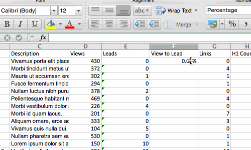
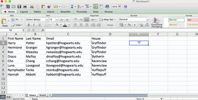
1. Use Pivot tables to recognize and make sense of data.
Pivot tables are used to reorganize data in a spreadsheet. They won’t change the data that you have, but they can sum up values and compare different information in your spreadsheet, depending on what you’d like them to do.
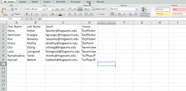
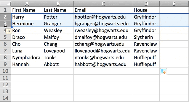
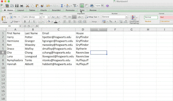
Let’s take a look at an example. Let’s say I want to take a look at how many people are in each house at Hogwarts. You may be thinking that I don’t have too much data, but for longer data sets, this will come in handy.
To create the Pivot Table, I go to Data > Pivot Table. If you’re using the most recent version of Excel, you’d go to Insert > Pivot Table. Excel will automatically populate your Pivot Table, but you can always change around the order of the data. Then, you have four options to choose from.
- Report Filter: This allows you to only look at certain rows in your dataset. For example, if I wanted to create a filter by house, I could choose to only include students in Gryffindor instead of all students.
- Column Labels: These would be your headers in the dataset.
- Row Labels: These could be your rows in the dataset. Both Row and Column labels can contain data from your columns (e.g. First Name can be dragged to either the Row or Column label — it just depends on how you want to see the data.)
- Value: This section allows you to look at your data differently. Instead of just pulling in any numeric value, you can sum, count, average, max, min, count numbers, or do a few other manipulations with your data. In fact, by default, when you drag a field to Value, it always does a count.
Since I want to count the number of students in each house, I’ll go to the Pivot table builder and drag the House column to both the Row Labels and the Values. This will sum up the number of students associated with each house.
2. Add more than one row or column.
As you play around with your data, you might find you’re constantly needing to add more rows and columns. Sometimes, you may even need to add hundreds of rows. Doing this one-by-one would be super tedious. Luckily, there’s always an easier way.
To add multiple rows or columns in a spreadsheet, highlight the same number of preexisting rows or columns that you want to add. Then, right-click and select «Insert.»
In the example below, I want to add an additional three rows. By highlighting three rows and then clicking insert, I’m able to add an additional three blank rows into my spreadsheet quickly and easily.
3. Use filters to simplify your data.
When you’re looking at very large data sets, you don’t usually need to be looking at every single row at the same time. Sometimes, you only want to look at data that fit into certain criteria.
That’s where filters come in.
Filters allow you to pare down your data to only look at certain rows at one time. In Excel, a filter can be added to each column in your data — and from there, you can then choose which cells you want to view at once.
Let’s take a look at the example below. Add a filter by clicking the Data tab and selecting «Filter.» Clicking the arrow next to the column headers and you’ll be able to choose whether you want your data to be organized in ascending or descending order, as well as which specific rows you want to show.
In my Harry Potter example, let’s say I only want to see the students in Gryffindor. By selecting the Gryffindor filter, the other rows disappear.
 Pro Tip: Copy and paste the values in the spreadsheet when a Filter is on to do additional analysis in another spreadsheet.
4. Remove duplicate data points or sets.
Larger data sets tend to have duplicate content. You may have a list of multiple contacts in a company and only want to see the number of companies you have. In situations like this, removing the duplicates comes in quite handy.
To remove your duplicates, highlight the row or column that you want to remove duplicates of. Then, go to the Data tab and select «Remove Duplicates» (which is under the Tools subheader in the older version of Excel). A pop-up will appear to confirm which data you want to work with. Select «Remove Duplicates,» and you’re good to go.
You can also use this feature to remove an entire row based on a duplicate column value. So if you have three rows with Harry Potter’s information and you only need to see one, then you can select the whole dataset and then remove duplicates based on email. Your resulting list will have only unique names without any duplicates.
5. Transpose rows into columns.
When you have rows of data in your spreadsheet, you might decide you actually want to transform the items in one of those rows into columns (or vice versa). It would take a lot of time to copy and paste each individual header — but what the transpose feature allows you to do is simply move your row data into columns, or the other way around.
Start by highlighting the column that you want to transpose into rows. Right-click it, and then select «Copy.» Next, select the cells on your spreadsheet where you want your first row or column to begin. Right-click on the cell, and then select «Paste Special.» A module will appear — at the bottom, you’ll see an option to transpose. Check that box and select OK. Your column will now be transferred to a row or vice-versa.
On newer versions of Excel, a drop-down will appear instead of a pop-up.

6. Split up text information between columns.
What if you want to split out information that’s in one cell into two different cells? For example, maybe you want to pull out someone’s company name through their email address. Or perhaps you want to separate someone’s full name into a first and last name for your email marketing templates.
Thanks to Excel, both are possible. First, highlight the column that you want to split up. Next, go to the Data tab and select «Text to Columns.» A module will appear with additional information.
First, you need to select either «Delimited» or «Fixed Width.»
- «Delimited» means you want to break up the column based on characters such as commas, spaces, or tabs.
- «Fixed Width» means you want to select the exact location on all the columns that you want the split to occur.
In the example case below, let’s select «Delimited» so we can separate the full name into first name and last name.
Then, it’s time to choose the Delimiters. This could be a tab, semi-colon, comma, space, or something else. («Something else» could be the «@» sign used in an email address, for example.) In our example, let’s choose the space. Excel will then show you a preview of what your new columns will look like.
When you’re happy with the preview, press «Next.» This page will allow you to select Advanced Formats if you choose to. When you’re done, click «Finish.»
7. Use formulas for simple calculations.
In addition to doing pretty complex calculations, Excel can help you do simple arithmetic like adding, subtracting, multiplying, or dividing any of your data.
- To add, use the + sign.
- To subtract, use the — sign.
- To multiply, use the * sign.
- To divide, use the / sign.
You can also use parentheses to ensure certain calculations are done first. In the example below (10+10*10), the second and third 10 were multiplied together before adding the additional 10. However, if we made it (10+10)*10, the first and second 10 would be added together first.
8. Get the average of numbers in your cells.
If you want the average of a set of numbers, you can use the formula =AVERAGE(Cell1:Cell2). If you want to sum up a column of numbers, you can use the formula =SUM(Cell1:Cell2).
9. Use conditional formatting to make cells automatically change color based on data.
Conditional formatting allows you to change a cell’s color based on the information within the cell. For example, if you want to flag certain numbers that are above average or in the top 10% of the data in your spreadsheet, you can do that. If you want to color code commonalities between different rows in Excel, you can do that. This will help you quickly see information that is important to you.
To get started, highlight the group of cells you want to use conditional formatting on. Then, choose «Conditional Formatting» from the Home menu and select your logic from the dropdown. (You can also create your own rule if you want something different.) A window will pop up that prompts you to provide more information about your formatting rule. Select «OK» when you’re done, and you should see your results automatically appear.
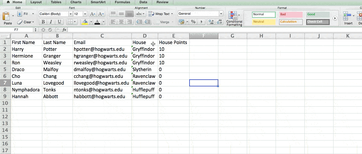
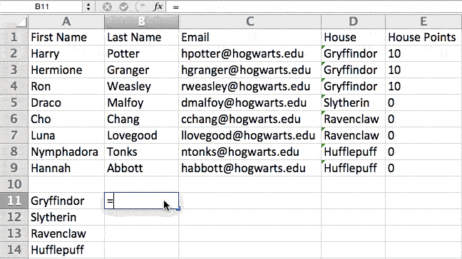
10. Use the IF Excel formula to automate certain Excel functions.
Sometimes, we don’t want to count the number of times a value appears. Instead, we want to input different information into a cell if there is a corresponding cell with that information.
For example, in the situation below, I want to award ten points to everyone who belongs in the Gryffindor house. Instead of manually typing in 10’s next to each Gryffindor student’s name, I can use the IF Excel formula to say that if the student is in Gryffindor, then they should get ten points.
The formula is: IF(logical_test, value_if_true, [value_if_false])
Example Shown Below: =IF(D2=»Gryffindor»,»10″,»0″)
In general terms, the formula would be IF(Logical Test, value of true, value of false). Let’s dig into each of these variables.
- Logical_Test: The logical test is the «IF» part of the statement. In this case, the logic is D2=»Gryffindor» because we want to make sure that the cell corresponding with the student says «Gryffindor.» Make sure to put Gryffindor in quotation marks here.
- Value_if_True: This is what we want the cell to show if the value is true. In this case, we want the cell to show «10» to indicate that the student was awarded the 10 points. Only use quotation marks if you want the result to be text instead of a number.
- Value_if_False: This is what we want the cell to show if the value is false. In this case, for any student not in Gryffindor, we want the cell to show «0». Only use quotation marks if you want the result to be text instead of a number.
Note: In the example above, I awarded 10 points to everyone in Gryffindor. If I later wanted to sum the total number of points, I wouldn’t be able to because the 10’s are in quotes, thus making them text and not a number that Excel can sum.
The real power of the IF function comes when you string multiple IF statements together, or nest them. This allows you to set multiple conditions, get more specific results, and ultimately organize your data into more manageable chunks.
Ranges are one way to segment your data for better analysis. For example, you can categorize data into values that are less than 10, 11 to 50, or 51 to 100. Here’s how that looks in practice:
=IF(B3<11,“10 or less”,IF(B3<51,“11 to 50”,IF(B3<100,“51 to 100”)))
It can take some trial-and-error, but once you have the hang of it, IF formulas will become your new Excel best friend.
11. Use dollar signs to keep one cell’s formula the same regardless of where it moves.
Have you ever seen a dollar sign in an Excel formula? When used in a formula, it isn’t representing an American dollar; instead, it makes sure that the exact column and row are held the same even if you copy the same formula in adjacent rows.
You see, a cell reference — when you refer to cell A5 from cell C5, for example — is relative by default. In that case, you’re actually referring to a cell that’s five columns to the left (C minus A) and in the same row (5). This is called a relative formula. When you copy a relative formula from one cell to another, it’ll adjust the values in the formula based on where it’s moved. But sometimes, we want those values to stay the same no matter whether they’re moved around or not — and we can do that by turning the formula into an absolute formula.
To change the relative formula (=A5+C5) into an absolute formula, we’d precede the row and column values by dollar signs, like this: (=$A$5+$C$5). (Learn more on Microsoft Office’s support page here.)
12. Use the VLOOKUP function to pull data from one area of a sheet to another.
Have you ever had two sets of data on two different spreadsheets that you want to combine into a single spreadsheet?
For example, you might have a list of people’s names next to their email addresses in one spreadsheet, and a list of those same people’s email addresses next to their company names in the other — but you want the names, email addresses, and company names of those people to appear in one place.
I have to combine data sets like this a lot — and when I do, the VLOOKUP is my go-to formula.
Before you use the formula, though, be absolutely sure that you have at least one column that appears identically in both places. Scour your data sets to make sure the column of data you’re using to combine your information is exactly the same, including no extra spaces.
The formula: =VLOOKUP(lookup value, table array, column number, Approximate match (TRUE) or Exact match (FALSE))
The formula with variables from our example below: =VLOOKUP(C2,Sheet2!A:B,2,FALSE)
In this formula, there are several variables. The following is true when you want to combine information in Sheet 1 and Sheet 2 onto Sheet 1.
- Lookup Value: This is the identical value you have in both spreadsheets. Choose the first value in your first spreadsheet. In the example that follows, this means the first email address on the list, or cell 2 (C2).
- Table Array: The table array is the range of columns on Sheet 2 you’re going to pull your data from, including the column of data identical to your lookup value (in our example, email addresses) in Sheet 1 as well as the column of data you’re trying to copy to Sheet 1. In our example, this is «Sheet2!A:B.» «A» means Column A in Sheet 2, which is the column in Sheet 2 where the data identical to our lookup value (email) in Sheet 1 is listed. The «B» means Column B, which contains the information that’s only available in Sheet 2 that you want to translate to Sheet 1.
- Column Number: This tells Excel which column the new data you want to copy to Sheet 1 is located in. In our example, this would be the column that «House» is located in. «House» is the second column in our range of columns (table array), so our column number is 2. [Note: Your range can be more than two columns. For example, if there are three columns on Sheet 2 — Email, Age, and House — and you still want to bring House onto Sheet 1, you can still use a VLOOKUP. You just need to change the «2» to a «3» so it pulls back the value in the third column: =VLOOKUP(C2:Sheet2!A:C,3,false).]
- Approximate Match (TRUE) or Exact Match (FALSE): Use FALSE to ensure you pull in only exact value matches. If you use TRUE, the function will pull in approximate matches.
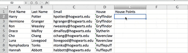
In the example below, Sheet 1 and Sheet 2 contain lists describing different information about the same people, and the common thread between the two is their email addresses. Let’s say we want to combine both datasets so that all the house information from Sheet 2 translates over to Sheet 1.
So when we type in the formula =VLOOKUP(C2,Sheet2!A:B,2,FALSE), we bring all the house data into Sheet 1.
Keep in mind that VLOOKUP will only pull back values from the second sheet that are to the right of the column containing your identical data. This can lead to some limitations, which is why some people prefer to use the INDEX and MATCH functions instead.
13. Use INDEX and MATCH formulas to pull data from horizontal columns.
Like VLOOKUP, the INDEX and MATCH functions pull in data from another dataset into one central location. Here are the main differences:
- VLOOKUP is a much simpler formula. If you’re working with large data sets that would require thousands of lookups, using the INDEX and MATCH function will significantly decrease load time in Excel.
- The INDEX and MATCH formulas work right-to-left, whereas VLOOKUP formulas only work as a left-to-right lookup. In other words, if you need to do a lookup that has a lookup column to the right of the results column, then you’d have to rearrange those columns in order to do a VLOOKUP. This can be tedious with large datasets and/or lead to errors.
So if I want to combine information in Sheet 1 and Sheet 2 onto Sheet 1, but the column values in Sheets 1 and 2 aren’t the same, then to do a VLOOKUP, I would need to switch around my columns. In this case, I’d choose to do an INDEX and MATCH instead.
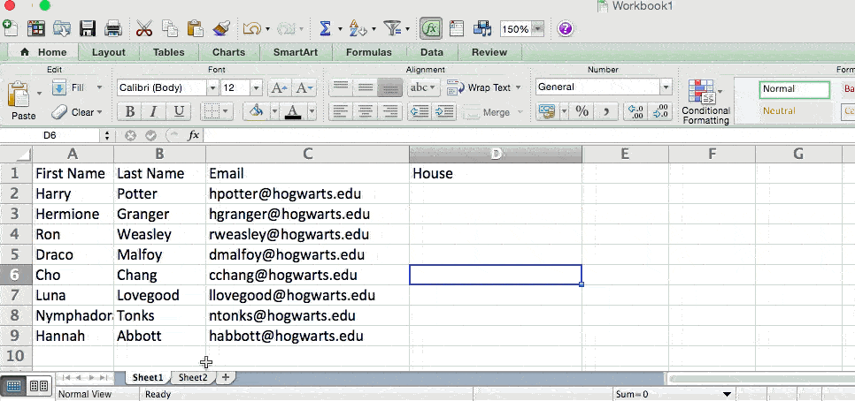
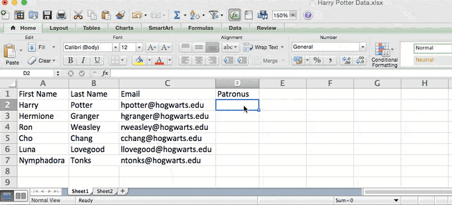
Let’s look at an example. Let’s say Sheet 1 contains a list of people’s names and their Hogwarts email addresses, and Sheet 2 contains a list of people’s email addresses and the Patronus that each student has. (For the non-Harry Potter fans out there, every witch or wizard has an animal guardian called a «Patronus» associated with him or her.) The information that lives in both sheets is the column containing email addresses, but this email address column is in different column numbers on each sheet. I’d use the INDEX and MATCH formulas instead of VLOOKUP so I wouldn’t have to switch any columns around.
So what’s the formula, then? The formula is actually the MATCH formula nested inside the INDEX formula. You’ll see I differentiated the MATCH formula using a different color here.
The formula: =INDEX(table array, MATCH formula)
This becomes: =INDEX(table array, MATCH (lookup_value, lookup_array))
The formula with variables from our example below: =INDEX(Sheet2!A:A,(MATCH(Sheet1!C:C,Sheet2!C:C,0)))
Here are the variables:
- Table Array: The range of columns on Sheet 2 containing the new data you want to bring over to Sheet 1. In our example, «A» means Column A, which contains the «Patronus» information for each person.
- Lookup Value: This is the column in Sheet 1 that contains identical values in both spreadsheets. In the example that follows, this means the «email» column on Sheet 1, which is Column C. So: Sheet1!C:C.
- Lookup Array: This is the column in Sheet 2 that contains identical values in both spreadsheets. In the example that follows, this refers to the «email» column on Sheet 2, which happens to also be Column C. So: Sheet2!C:C.
Once you have your variables straight, type in the INDEX and MATCH formulas in the top-most cell of the blank Patronus column on Sheet 1, where you want the combined information to live.
14. Use the COUNTIF function to make Excel count words or numbers in any range of cells.
Instead of manually counting how often a certain value or number appears, let Excel do the work for you. With the COUNTIF function, Excel can count the number of times a word or number appears in any range of cells.
For example, let’s say I want to count the number of times the word «Gryffindor» appears in my data set.
The formula: =COUNTIF(range, criteria)
The formula with variables from our example below: =COUNTIF(D:D,»Gryffindor»)
In this formula, there are several variables:
- Range: The range that we want the formula to cover. In this case, since we’re only focusing on one column, we use «D:D» to indicate that the first and last column are both D. If I were looking at columns C and D, I would use «C:D.»
- Criteria: Whatever number or piece of text you want Excel to count. Only use quotation marks if you want the result to be text instead of a number. In our example, the criteria is «Gryffindor.»
Simply typing in the COUNTIF formula in any cell and pressing «Enter» will show me how many times the word «Gryffindor» appears in the dataset.
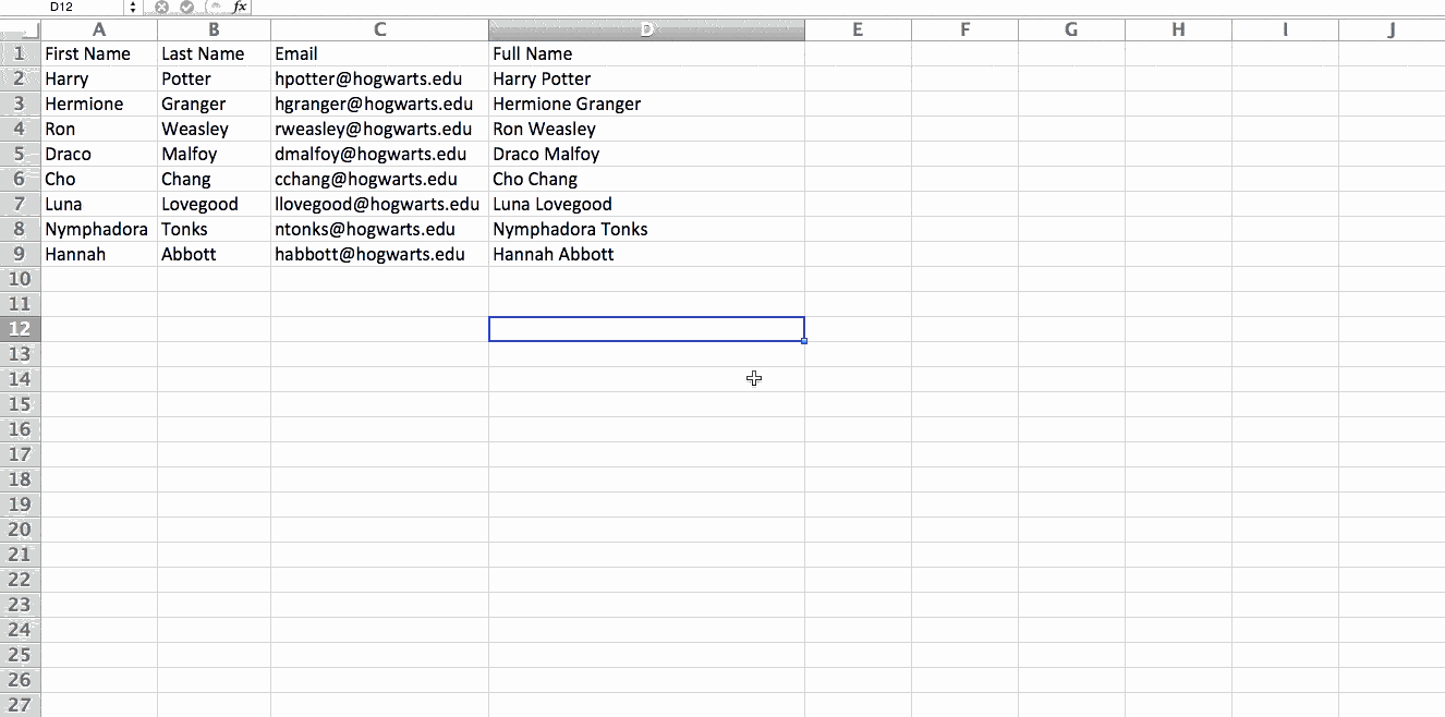
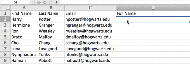
15. Combine cells using &.
Databases tend to split out data to make it as exact as possible. For example, instead of having a column that shows a person’s full name, a database might have the data as a first name and then a last name in separate columns. Or, it may have a person’s location separated by city, state, and zip code. In Excel, you can combine cells with different data into one cell by using the «&» sign in your function.
The formula with variables from our example below: =A2&» «&B2
Let’s go through the formula together using an example. Pretend we want to combine first names and last names into full names in a single column. To do this, we’d first put our cursor in the blank cell where we want the full name to appear. Next, we’d highlight one cell that contains a first name, type in an «&» sign, and then highlight a cell with the corresponding last name.
But you’re not finished — if all you type in is =A2&B2, then there will not be a space between the person’s first name and last name. To add that necessary space, use the function =A2&» «&B2. The quotation marks around the space tell Excel to put a space in between the first and last name.
To make this true for multiple rows, simply drag the corner of that first cell downward as shown in the example.
16. Add checkboxes.
If you’re using an Excel sheet to track customer data and want to oversee something that isn’t quantifiable, you could insert checkboxes into a column.
For example, if you’re using an Excel sheet to manage your sales prospects and want to track whether you called them in the last quarter, you could have a «Called this quarter?» column and check off the cells in it when you’ve called the respective client.
Here’s how to do it.
Highlight a cell you’d like to add checkboxes to in your spreadsheet. Then, click DEVELOPER. Then, under FORM CONTROLS, click the checkbox or the selection circle highlighted in the image below.
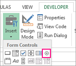
Once the box appears in the cell, copy it, highlight the cells you also want it to appear in, and then paste it.
17. Hyperlink a cell to a website.
If you’re using your sheet to track social media or website metrics, it can be helpful to have a reference column with the links each row is tracking. If you add a URL directly into Excel, it should automatically be clickable. But, if you have to hyperlink words, such as a page title or the headline of a post you’re tracking, here’s how.
Highlight the words you want to hyperlink, then press Shift K. From there a box will pop up allowing you to place the hyperlink URL. Copy and paste the URL into this box and hit or click Enter.
If the key shortcut isn’t working for any reason, you can also do this manually by highlighting the cell and clicking Insert > Hyperlink.
18. Add drop-down menus.
Sometimes, you’ll be using your spreadsheet to track processes or other qualitative things. Rather than writing words into your sheet repetitively, such as «Yes», «No», «Customer Stage», «Sales Lead», or «Prospect», you can use dropdown menus to quickly mark descriptive things about your contacts or whatever you’re tracking.
Here’s how to add drop-downs to your cells.
Highlight the cells you want the drop-downs to be in, then click the Data menu in the top navigation and press Validation.
From there, you’ll see a Data Validation Settings box open. Look at the Allow options, then click Lists and select Drop-down List. Check the In-Cell dropdown button, then press OK.
19. Use the format painter.
As you’ve probably noticed, Excel has a lot of features to make crunching numbers and analyzing your data quick and easy. But if you ever spent some time formatting a sheet to your liking, you know it can get a bit tedious.
Don’t waste time repeating the same formatting commands over and over again. Use the format painter to easily copy the formatting from one area of the worksheet to another. To do so, choose the cell you’d like to replicate, then select the format painter option (paintbrush icon) from the top toolbar.
Excel Keyboard Shortcuts
Creating reports in Excel is time-consuming enough. How can we spend less time navigating, formatting, and selecting items in our spreadsheet? Glad you asked. There are a ton of Excel shortcuts out there, including some of our favorites listed below.
Create a New Workbook
PC: Ctrl-N | Mac: Command-N
Select Entire Row
PC: Shift-Space | Mac: Shift-Space
Select Entire Column
PC: Ctrl-Space | Mac: Control-Space
Select Rest of Column
PC: Ctrl-Shift-Down/Up | Mac: Command-Shift-Down/Up
Select Rest of Row
PC: Ctrl-Shift-Right/Left | Mac: Command-Shift-Right/Left
Add Hyperlink
PC: Ctrl-K | Mac: Command-K
Open Format Cells Window
PC: Ctrl-1 | Mac: Command-1
Autosum Selected Cells
PC: Alt-= | Mac: Command-Shift-T
Other Excel Help Resources
- How to Make a Chart or Graph in Excel [With Video Tutorial]
- Design Tips to Create Beautiful Excel Charts and Graphs
- Totally Free Microsoft Excel Templates That Make Marketing Easier
- How to Learn Excel Online: Free and Paid Resources for Excel Training
Use Excel to Automate Processes in Your Team
Even if you’re not an accountant, you can still use Excel to automate tasks and processes in your team. With the tips and tricks we shared in this post, you’ll be sure to use Excel to its fullest extent and get the most out of the software to grow your business.
Editor’s Note: This post was originally published in August 2017 but has been updated for comprehensiveness.

As a topmost spreadsheet application on this planet, Microsoft Excel has a lot of benefits for anyone who knows how to use it.
And if you are one of those people who want to learn it and wondering how this can help you in your work, when I have listed the top ten benefits of Microsoft Excel here.
- Best way to store data
- You can perform calculations
- All the tools for data analysis
- Easy to data visualizations with charts
- You can print reports easily
- So many free templates to use
- You can code to automate
- Transform and clean data
- Store data with millions of rows
- You can work with Excel online + mobile app
Don’t forget to download this EXCEL PRODUCTIVITY BUNDLE (E-BOOKS) from here to level up your EXCEL SKILLS this year.
1. The Best Way to Store Data
Even if you don’t use any of the options or any tool which Excel offers you, it is the best way to store data. Why I’m saying this because Excel is a kind of application that is used by millions of people.

So when you store data in Excel and then share it with others, they can access it easily.
2. You can perform calculations
What makes Excel the best spreadsheet application on the planet is its ability to perform calculations. In Excel, you have a complete list of functions that you can use for the calculations.

Basically, an Excel function is a predefined formula that returns a specific result based on the values you specify.
But apart from that, you can also create your own formulas by combining two or more functions or just by performing calculations using operators.
- 100+ Excel Formulas List
- 100+ Excel Functions List
Quick Formulas: Calculate Time Difference – Compound Interest – Count Cells with Text – Count Unique Values – Quarter Formula
3. All the tools for data analysis
The core motive of having data is to analyze and get insights out of it. The good news is Excel has some of the most powerful tools to analyze data.
Imagine you have data with thousands of rows, you can insert a pivot table out of that data and create a summary table.

Some of the things you can do with pivot tables to analyze data: Grouping Dates in a Pivot Table – Conditional Formatting in a Pivot Table – Rank Column in a Pivot Table – Add a Date Timeline in a Pivot Table – Running Total Column in a Pivot Table
4. Easy to Create Data Visualizations with Charts
In Excel, you have all those options to create charts and present your data in a visual way.
All those major types of charts that you need to use to present your data are already there and you can insert them with a single click.
If you go to the Insert Tab, in the charts group, you can find all the charts which you can insert.

Not just that, there’s also a button called recommended charts that you can use to let Microsoft Excel recommend you the best possible chart to use for the data you have in your worksheet.

And if you think that you need something other than the default charts you have the option to create advanced charts using some specific methods.
Here we have a list of the top 10 ADVANCED EXCEL CHARTS that you can use in Excel. And you can also create in-cell charts to make your data easily understandable for anyone.
5. You can Print Reports Easily
Even if you are a person who likes to save trees but there could be a point where you need to print reports to share with others or present them to someone.
Well, Excel allows you to print with a lot of customization where you can change the margin, paper size, orientation, etc.

There are a whole bunch of options that you can use for page setup before printing a report.
6. So many free templates to use
One of the most popular things about Excel is you can create dashboards and templates.

There are a whole bunch of free templates that you can download and use.
Free Excel Templates to Start with
- Excel Inventory Template with Formulas
- Sales Template
- Expense Tracker
7. You can code to automate
Microsoft Office has its own coding language which is called VBA (visual basic for applications) and it allows you to write code for almost all the activities that you perform manually in Excel.

You can automate all kinds of activities from simple (make a text bold) to complex (insert a pivot table) using a VBA code.
Start Learning VBA
- Excel VBA Tutorial (Chapter-by-Chapter Guide)
- Macro Examples + Free PDF
- VBA IF
- VBA Message Box
- Personal Macro Workbook
- VBA Functions
Once you learn the basics of VBA, you can also create a custom function by writing code.
8. Transform and clean data
If you are one of those people who work with data a lot or you know someone who works, there are a lot of situations where you need to deal with messy data which you need to clean before you use it.
The process of cleaning and transforming data takes a big chunk of your time and it can be a tedious process.
For this, Microsoft has introduced the power query which is a data transformation and cleaning engine well you can load data from multiple sources, transform it, and then load it back to the worksheet.
What makes power query such a powerful tool? Check out this complete POWER QUERY guide to understand.
9. Store data with millions of rows
Well, there is no limit to data, but Excel has a limit in terms of rows and columns. So that’s why Microsoft came up with Power Pivot where you can store data with millions of rows and then you can perform calculations within Power Pivot.

See this (Power Pivot – Overview and Learning)
10. You can work with Excel online + mobile app
As most companies these days are moving to the cloud and Microsoft Excel has its own web version. It has so many features, like functions, pivot tables, and pivot charts just like the desktop app.

And recently Microsoft has launched its all-in-one office app that you can use to work on spreadsheets and mobile as well.

Start your Excel Learning.
![]()
Download Article
![]()
Download Article
Are you new to Microsoft Excel and need to work on a spreadsheet? Excel is so overrun with useful and complicated features that it might seem impossible for a beginner to learn. But don’t worry—once you learn a few basic tricks, you’ll be entering, manipulating, calculating, and graphing data in no time! This wikiHow tutorial will introduce you to the most important features and functions you’ll need to know when starting out with Excel, from entering and sorting basic data to writing your first formulas.
Things You Should Know
- Use Quick Analysis in Excel to perform quick calculations and create helpful graphs without any prior Excel knowledge.
- Adding your data to a table makes it easy to sort and filter data by your preferred criteria.
- Even if you’re not a math person, you can use basic Excel math functions to add, subtract, find averages and more in seconds.
-

1
Create or open a workbook. When people refer to «Excel files,» they are referring to workbooks, which are files that contain one or more sheets of data on individual tabs. Each tab is called a worksheet or spreadsheet, both of which are used interchangeably. When you open Excel, you’ll be prompted to open or create a workbook.
- To start from scratch, click Blank workbook. Otherwise, you can open an existing workbook or create a new one from one of Excel’s helpful templates, such as those designed for budgeting.
-
2
Explore the worksheet. When you create a new blank workbook, you’ll have a single worksheet called Sheet1 (you’ll see that on the tab at the bottom) that contains a grid for your data. Worksheets are made of individual cells that are organized into columns and rows.
- Columns are vertical and labeled with letters, which appear above each column.
- Rows are horizontal and are labeled by numbers, which you’ll see running along the left side of the worksheet.
- Every cell has an address which contains its column letter and row number. For example, the top-left cell in your worksheet’s address is A1 because it’s in column A, row 1.
- A workbook can have multiple worksheets, all containing different sets of data. Each worksheet in your workbook has a name—you can rename a worksheet by right-clicking its tab and selecting Rename.
- To add another worksheet, just click the + next to the worksheet tab(s).
Advertisement
-
3
Save your workbook. Once you save your workbook once, Excel will automatically save any changes you make by default.[1]
This prevents you from accidentally losing data.- Click the File menu and select Save As.
- Choose a location to save the file, such as on your computer or in OneDrive.
- Type a name for your workbook. All workbooks will automatically inherit the the .XLSX file extension.
- Click Save.


Advertisement
-
1
Click a cell to select it. When you click a cell, it will highlight to indicate that it’s selected.
- When you type something into a cell, the input text is called a value. Entering data into Excel is as simple as typing values into each cell.
- When entering data, the first row of your worksheet (e.g., A1, B1, C1) is typically used as headers for each column. This is helpful when creating graphs or tables which require labels.
- For example, if you’re adding a list of dates in column A, you might click cell A1 and type Date into the cell as the column header.
-
2
Type a word or number into the cell. As you’re typing, you’ll see the letters and/or numbers appear in the cell, as well as in the formula bar at the top of the worksheet.
- When you start practicing more advanced Excel features like creating formulas, this bar will come in handy.
- You can also copy and paste text from other applications into your worksheet, tables from PDFs and the web.
-
3
Press ↵ Enter or ⏎ Return. This enters the data into the cell and moves to the next cell in the column.
-
4
Automatically fill columns based on existing data. Let’s say you want to make a list of consecutive dates or numbers. Or what if you want to fill a column with many of the same values that follow a pattern? As long as Excel can recognize some sort of pattern in your data, such as a particular order, you can use Autofill to automatically populate data into the rest of your column. Here’s a trick to see it in action.
- In a blank column, type 1 into the first cell, 2 into the second cell, and then 3 into the third cell.
- Hover your mouse cursor over the bottom-right corner of the last cell in your series—it will turn to a crosshair.
- Click and drag the crosshair down the column, then release the mouse button once you’ve gone down as far as you like. By default, this will fill the remaining cells with the value of the selected cell—at this point, you’ll probably have something like 1, 2, 3, 3, 3, 3, 3, 3.
- Click the small icon at the bottom-right corner of the filled data to open AutoFill options, and select Fill Series to automatically detect the series or pattern. Now you’ll have a list of consecutive numbers. Try this cool feature out with different patterns!
- Once you get the hang of AutoFill, you’ll have to try flash fill, which you can use to join two columns of data into a single merged column.
-
5
Adjust the column sizes so you can see all of the values. Sometimes typing long values into a cell hides the value and displays hash symbols ### instead of what you’ve typed. If you want to be able to see everything, you can snap the cell contents to the width of the widest cell. For example, let’s say we have some long values in column B:
- To expand the contents of column B, hover the cursor over the dividing line between the B and C at the top of the worksheet—once your cursor is right on the line, it will turn to two arrows pointing in either direction.[2]
- Click and drag the separator until the column is wide enough to accommodate your data, or just double-click the separator to instantly snap the column to the size of the widest value.
- To expand the contents of column B, hover the cursor over the dividing line between the B and C at the top of the worksheet—once your cursor is right on the line, it will turn to two arrows pointing in either direction.[2]
-
6
Wrap text in a cell. If your longer values are now awkwardly long, you can enable text wrapping in one or more cells. Just click a cell (or drag the mouse to select multiple cells), click the Home tab, and then click Wrap Text on the toolbar.
-
7
Edit a cell value. If you need to make a change to a cell, you can double-click the cell to activate the cursor, and then make any changes you need. When you’re finished, just press Enter or Return again.
- To delete the contents of a cell, click the cell once and press delete on your keyboard.
-
8
Apply styles to your data. Whether you want to highlight certain values with color so they stand out or just want to make your data look pretty, changing the colors of cells and their containing values is easy—especially if you’re used to Microsoft Word:
- Select a cell, column, row, or multiple cells at once.
- On the Home tab, click Cell Styles if you’d like to quickly apply quick color styles.
- If you’d rather use more custom options, right-click the selected cell(s) and select Format Cells. Then, use the colors on the Fill tab to customize the cell’s background, or the colors on the Font tab for value colors.
-
9
Apply number formatting to cells containing numbers. If you have data that contains numbers such as prices, measurements, dates, or times, you can apply number formatting to the data so it will display consistently.[3]
By default, the number format is General, which means numbers display exactly as you type them.- Select the cell you want to format. If you’re working with an entire column or row, you can just click the column letter or row number to select the whole thing.
- On the Home tab, click the drop-down menu at the top-center—it’ll say General by default, unless you selected cells that Excel recognizes as a different type of number like Currency or Time.
- Choose one of the formatting options in the list, such as Short Date or Percentage, or click More Number Formats at the bottom to expand all options (we recommend this!).
- If you selected More Number Formats, the Format Cells dialog will expand to the Number tab, where you’ll see several categories for number types.
- Select a category, such as Currency if working with money, or Date if working with dates. Then, choose your preferences, such as a currency symbol and/or decimal places.
- Click OK to apply your formatting.


Advertisement
-
1
Select all of the data you’ve entered so far. Adding your data to a table is the easiest way to work with and analyze data.[4]
Start by highlighting the values you’ve entered so far, including your column headers. Tables also make it easy to sort and filter your data based on values.- Tables traditionally apply different or alternating colors to every other row for easy viewing. Many table options also add borders between cells and/or columns and rows.
-
2
Click Format as Table. You’ll see this at the top-center part of the Home tab.[5]
-
3
Select a table style. Choose any of Excel’s default table styles to get started. You’ll see a small window titled «Create Table» once selected.
- Once you get the hang of tables, you can return here to customize your table further by selecting New Table Style.
-
4
Make sure «My table has headers» is selected and click OK. This tells Excel to turn your column headers into drop-down menus that you can easily sort and filter. Once you click OK, you’ll see that your data now has a color scheme and drop-down menus.
-
5
Click the drop-down menu at the top of a column. Now you’ll see options for sorting that column, as well as several options for filtering all of your data based on its values.
-
6
Choose which data to display based on values in this column. The simplest way to do this is to uncheck the values you don’t want to display—if you uncheck a particular date, for example, you’ll prevent rows that contain the selected date in from appearing in your data. You can also use Text Filters or Number Filters, depending on the type of data in the column:
- If you chose a numerical column, select Number Filters, then choose an option like Greater Than… or Does Not Equal to be extra specific about which values to hide.
- For text columns, you can choose Text Filters, where you can specify things like Begins with or Contains.
- You can also filter by cell color.
-
7
Click OK. Your data is now filtered based on your selections. You’ll also see a small funnel icon in the drop-down menu, which indicates that the data is filtering out certain values.
- To unfilter your data, click the funnel icon, click Clear filter from (column name), and then click OK.
- You can also filter columns that aren’t in tables. Just select a column and click Filter on the Data tab to add a drop-down to that column.
-
8
Sort your data in ascending or descending order. Click the drop-down arrow at the top of a column to view sorting options—these allow you to sort all of your data in order based on the current column.
- If you’re working with numbers, click Smallest to Largest to sort in ascending order, or Largest to Smallest for descending order.[6]
- If you’re working with text values, Sort A to Z will sort in ascending order, while Sort Z to A will sort in reverse.
- When it comes to sorting dates and times, Sort Oldest to Newest will sort with the earliest date at the top and the oldest date at the bottom, and Newest to Oldest displays the dates in descending order.
- When you sort a column, all other columns in the table adjust based on the sort.
- If you’re working with numbers, click Smallest to Largest to sort in ascending order, or Largest to Smallest for descending order.[6]


Advertisement
-
1
Select the data in your worksheet. Excel’s Quick Analysis feature is the easiest way to perform basic calculations (including totals, averages, and counts) and create meaningful tables or graphs without the need for advanced Excel knowledge.[7]
Use your mouse to select your data (including your column headers) to get started. -
2
Click the Quick Analysis icon. This is the small icon that pops up at the bottom-right corner of your selection. It looks like a window with some colored lines.
-
3
Select an analysis type. You’ll see several tabs running along the top of the window, each of which gives you different option for visualizing your data:
- For math calculations, click the Totals tab, where you can select Sum, Average, Count, %Total, or Running Total. You’ll be able to choose whether to display the results at the bottom of each column or to the right.
- To create a chart, click the Charts tab, then select a chart to visualize your data. Before you settle on a chart, just hover the cursor over each option to see a preview.
- To add quick chart data to individual cells, click the Sparklines tab and choose a format. Again, you can hover the cursor over each option to see a preview.
- To instantly apply conditional formatting (which is usually a little more complex in Excel) based on your data, use the Formatting tab. Here you can choose an option like Color or Data Bars, which apply colors to your data based on trends.


Advertisement
-
1
Quickly add data with AutoSum. AutoSum is a built-in Excel function that makes it easy to find the total of one or more columns in a few clicks. Functions or formulas that perform calculations and other tasks based on the values of cells. When you use a function to get something done, you’re creating a formula, which is like a math equation. If you have a column or row of numbers you want to add:
- Click the cell below the numbers you want to add (if a column) or to the right (if a row).[8]
- On the Home tab, click AutoSum toward the upper-right corner of the app. A formula beginning with =SUM(cell+cell) will appear in the field, and a dotted line will surround the numbers you’re adding.
- Press Enter or Return. You should now see the total of the numbers in the selected field. This is here because you created your first formula—which you didn’t have to write by hand!
- If you change any numbers in your data after using AutoSum, the AutoSum value will update automatically.
- Click the cell below the numbers you want to add (if a column) or to the right (if a row).[8]
-
2
Write a simple math formula. AutoSum is just the beginning—Excel is famous for its ability to do all sorts of simple and complex math calculations on data. Fortunately, you don’t have to be a math whiz to create simple formulas to create everyday math formulas, like adding, subtracting, and multiplying. Here’s some basic formulas to get you started:
-
Add: — Type =SUM(cell+cell) (e.g.,
=SUM(A3+B3)) to add two cells’ values together, or type =SUM(cell,cell,cell) (e.g.,=SUM(A2,B2,C2)) to add a series of cell values together.- If you want to add all of the numbers in a whole column (or in a section of a column), type =SUM(cell:cell) (e.g.,
=SUM(A1:A12)) into the cell you want to use to display the result.
- If you want to add all of the numbers in a whole column (or in a section of a column), type =SUM(cell:cell) (e.g.,
-
Subtract: Type =SUM(cell-cell) (e.g.,
=SUM(A3-B3)) to subtract one cell value from another cell’s value. -
Divide: Type =SUM(cell/cell) (e.g.,
=SUM(A6/C5)) to divide one cell’s value by another cell’s value. -
Multiply: Type =SUM(cell*cell) (e.g.,
=SUM(A2*A7)) to multiply two cell values together.
-
Add: — Type =SUM(cell+cell) (e.g.,


Advertisement
-
1
Select a cell for an advanced formula. What if you need to do something more complicated than just adding numbers? Even if you don’t know how to write formulas by hand, you can still create useful formulas that work with your data in various ways. Start by clicking the cell in which you want to display your formula.
-
2
Click the Formulas tab. It’s a tab at the top of the Excel window.
-
3
Explore the Function Library. Several function categories appear in the toolbar, such as Financial, Text, and Math & Trig. Click the options to check out the types of functions available, though they might not make a whole lot of sense just yet.
-
4
Click Insert Function. This option is in the far-left side of the Formulas toolbar. This opens the Insert Function window, which gives you a more detailed breakdown of each function.
-
5
Click a function to learn about it. You can type what you want to do (such as round), or choose a category to filter the list of functions. Then, click any function to read a description of how it works and view its syntax.
- For example, to select the formula for finding the tangent of an angle, you would scroll down and click the TAN option.
-
6
Select a function and click OK. This creates a formula based on the selected function.
-
7
Fill out the function’s formula. When prompted, type in the number or select a cell for which you want to use the formula.
- For example, if you select the TAN function, you’ll type in the number for which you want to find the tangent, or select the cell that contains that number.
- Depending on your selected function, you may need to click through a couple of on-screen prompts.
-
8
Press ↵ Enter or ⏎ Return to run the formula. Doing so applies your function and displays it in your selected cell.


Advertisement
-
1
Set up the chart’s data. If you’re creating a line graph or a bar graph, for example, you’ll want to use one column of cells for the horizontal axis and one column of cells for the vertical axis. The best way to do this is to place your data in a table.
- Typically speaking, the left column is used for the horizontal axis and the column immediately to the right of it represents the vertical axis.
-
2
Select the data in your table. Click and drag your mouse from the top-left cell of the data down to the bottom-right cell of the data.
-
3
Click the Insert tab. It’s a tab at the top of the Excel window.
-
4
Click Recommended Charts. You’ll find this option in the «Charts» section of the Insert toolbar. A window with different chart templates will appear.
-
5
Select a chart template. Click the chart template you want to use based on the type of data you’re working with. If you don’t see a chart type you like, click the All Charts tab to explore by category, such as Pie, Bar, and X Y Scatter.
-
6
Click OK. It’s at the bottom of the window. This creates your chart.
-
7
Use the Chart Design tab to customize your chart. Any time you click your chart, the Chart Design tab will appear at the top of Excel. You can adjust the chart style here, change colors, and add additional elements.
-
8
Double-click a chart element to manage it in the Format panel. When you double-click something on your chart, such as a value, line, or bar, you’ll see options you can edit in the panel on the right side of excel. Here you can change the axis labels, alignment, and legend data.


Advertisement
Add New Question
-
Question
How do you add a check mark or an X mark to a cell?

You can go into Insert, then Symbol, and choose the symbol you want. After that, you can just copy and paste the symbol from one cell to another.
-
Question
Can I add work sheets on Excel?
Yes. At the bottom left of the Excel you will see the list of sheets. To the left of those sheets you will find a «+» sign. Click on it.
-
Question
How do I move cell contents to another cell?
Highlight the cell, right-click, and click Copy. Click destination cell, right-click and Paste.
See more answers
Ask a Question
200 characters left
Include your email address to get a message when this question is answered.
Submit
Advertisement
Video
Thanks for submitting a tip for review!
References
About This Article
Article SummaryX
1. Purchase and install Microsoft Office.
2. Enter data into individual cells.
3. Format cells based on certain criteria.
4. Organize data into rows and columns.
5. Perform math operations using formulas.
6. Use the Formulas tab to find additional formulas.
7. Use data to create charts.
8. Import data from other sources.
Did this summary help you?
Thanks to all authors for creating a page that has been read 646,263 times.
Reader Success Stories
-

«I am applying for a job that requires comprehensive knowledge of Excel. Well, I don’t have it, but this article…» more
Is this article up to date?
Before I get into the Google Sheet vs Excel debate, there is something you need to know.
I love Excel spreadsheets, and I have been an active user for 12+ years, and I use it every day. But at the same time, I am also a massive fan of Google Sheets. I run my online business using Google Sheets and Google Drive, so I have been using them more and more lately.
So, I believe that I can be objective in my comparison of Google Sheets and Excel. I see both these are Excellent spreadsheet tools, and I am excited to see how these develop in the coming years.
Also, this article is not about judging a winner. Both are great tools with pros and cons. Based on what you want to get done, you need to analyze the functionalities and choose what suits you best.
Enough of disclaimers, let’s get started with our Google Sheets vs Excel comparison!
Pros and Cons of Google Sheets vs Excel
|
Pros |
Cons |
|
|
Google Sheets |
Free |
Limited data visualization |
|
Collaborative by design |
Formulas are less customizable |
|
|
Realtime chat and revision history |
Slow load times on large spreadsheets |
|
|
Microsoft Excel |
Advanced functions |
More difficult to use |
|
Fast |
Collaboration is harder |
|
|
Superior charting options |
Costs money |
Key Differences Between Excel and Google Sheets
Is Google spreadsheet the same as Excel? No, not really. They are both spreadsheet software, but there is a lot of difference between Excel and Google Sheets. Here are the key differences between Excel and Google Sheets:
- Google Sheets is a purely online spreadsheet while Microsoft Excel is a desktop spreadsheet—although it does have an internet version.
- Google Sheets is a free spreadsheet and you can use all its features for free. It also has a business subscription for $5. On the other hand, Microsoft Excel is not free since it is a licensed product but comes in the Microsoft Office 365 package
- Another key difference between Excel and Google spreadsheets is that Google Sheets has simultaneous collaboration, which Excel does not have. In Google Sheets, you can share files and edit them in real-time with other people, while in Excel you can only track changes.
- Google Sheets automatically saves your files in your drive while Microsoft Excel automatically saves your spreadsheets to one drive or share point. For Microsoft Excel, however, you will need to set this up otherwise you will have to save your Excel files manually.
- Excel formulas and Google Sheets formulas also differ. They share the main functions but Excel has some advanced functions like XLOOKUP, while Google Sheets also has its own special functions like Google functions.
- The scripting language for Google Sheets is the Google Apps Script, while Microsoft Excel uses VBE.
- Excel can work with a large volume of data in millions while Google Sheets can only work with low volumes of data
Easy Comparison Tools for Microsoft Excel Vs Google Sheets
We’ve gone out of our way to build easy-to-understand diagrams to compare Google spreadsheets vs Excel. You can use this flow chart and table to identify the difference between Google Sheets and Excel and pick which suits you best.
Google Sheets Vs Microsoft Excel Flowchart

Google Sheets Vs Excel Comparison Table
|
Comparison Area |
Google Sheets |
Excel |
|
Cost of the Spreadsheet Tool |
✅ |
|
|
Features and Functionalities |
✅ |
|
|
Collaboration |
✅ |
|
|
Formulas |
✅ |
✅ |
|
Keyboard Shortcuts (and Mouse Shortcuts) |
✅ |
|
|
Data Analysis |
✅ |
|
|
Charting |
✅ |
✅ |
|
Automation (Visual Basic in Excel and Scripts in Google Sheets) |
✅ |
✅ |
|
Advanced Functionalities (Add-ins) |
✅ |
|
|
Releasing Updates |
✅ |
Google Spreadsheet vs Excel – Cost
Winner: Google Sheets
Why: It’s Free!
Cost is often one of the first determinants (and sometimes the most important) when selecting a spreadsheet program.
Microsoft Excel has a cost associated with it, and you can buy only Excel as a standalone tool or buy the Microsoft 365 subscription. But in any case, you will be charged monthly or yearly for it.
At the time of writing this article, Microsoft 365 subscription would cost you $70 a year. And if you only want Excel, it will be $159.99 (one time). Excel does now offer a free online version too, but lacks the features of the 365 subscription version.
On the contrary, Google Sheets is absolutely free to use. If you have a Google account (which many of us have because of using Gmail), then you already have access to Google Sheets.
While Google offers paid G-suite services, you can get the same Google Sheets functionality even if you are using the free version.
This is why many freelancers and small companies prefer using Google Sheets.
This is also a great strategy by Google as many students, teachers, and small companies, who cannot afford to pay for Microsoft Excel, start with Google Sheets and other Google products.
And once you are used to a specific spreadsheet program, you would try and stick to it in most cases.
So if the cost is the criteria, Google Sheets is the clear winner
The Difference Between Excel and Google Sheets Features and Functionalities
Winner: Excel
Why: It comes loaded with more functions and works a little faster
Because Excel is a tool that you can download and use on your own system, it can afford to have a lot more features than Google Sheets (which is web-based).
Excel uses the processing power of your laptop or desktop, while Google Sheets has to use the Internet connection and the servers on Google to get the same thing done (which makes it a bit slower).
This means that Excel can have better functionalities in the tool while Google Sheets would be slightly slower and would not have so many functionalities (unless, of course, they decide to come up with their own desktop app version)
Excel has also been around for a lot longer compared to Google Sheets. As a result, it has benefited from all the feedback from its users.
To give you some examples, Excel has a lot better functionalities for stuff such as Conditional Formatting or Pivot tables, or Data Analysis.
Collaboration
Winner: Google Sheets
Why: Most collaborative workplaces already use Google Sheets, and as it’s solely online, it’s easy to share spreadsheets.
If being a web-based tool is a drawback for Google Sheets when it comes to features and functionalities, it’s a huge plus when it comes to collaboration.
The level of collaboration that you can do with Google Sheets is way ahead of Excel.
While Excel has been making progress in enabling collaboration and making it easier for people to use it, it’s still not as smooth (or friction-less as they call it) as Google Sheets.
For example, if you need to collaborate with someone using Excel, these Excel files need to be saved on OneDrive or SharePoint.
While these tools may be used by big enterprise clients, most of the people are used to Google Drive, which is where you save your Google Sheets.
Collaboration in Google Sheets works seamlessly where you can have multiple users editing the same sheet from multiple devices (be it a desktop, laptop, tablet, or mobile).
You also don’t need to worry about saving your Google Sheets files as it is saved in real-time. You also get this with Excel in Microsoft 365, but it’s not something you would have if you were using the older versions.
All in all, Google Sheets has an upper hand when it comes to collaboration.
Formulas
Winner: Tie
Why: Both programs use lots of formulas and while one may be ahead at any one time, it doesn’t take long for the other to catch up.
When it comes to formulas, I find Excel and Google Sheets are neck to neck.
But if you force me to choose the winner, I would go with Google Sheets. To begin with, Google Sheets has more formulas as compared with Excel. Also, because it’s made as a web-based tool, it has some formulas that can work with the web.
For example, there is a formula called IMAGE in Google Sheets that you can directly insert an image in a cell using its URL.
Also, Google Sheets came up with dynamic arrays formulas such as SORT, FILTER, and UNIQUE a lot earlier than Excel did.
And while Excel in Microsoft 365 has these new formulas, these are not available to people who are not using Microsoft 365 (Excel 2016 or 2013 or prior versions).
But in the case of Google Sheets, everyone has access to these new formulas (and everyone gets access to all the new functionalities as soon as it’s released).
While Excel has been playing catch up in the formulas areas, they have recently started working on newer formulas that are not there in Google Sheets. For example, there is a new lookup formula called XLOOKUP, and they also added a new formula called LET, which is quite useful.
I believe both Google Sheets and Excel will continue to work on the formulas and at the same time continue to copy each other.
Keyboard Shortcuts (and Mouse Shortcuts)
Winner: Excel
Why: Sometimes, the browser shortcuts get in the way of Sheets shortcuts
Excel is a clear winner when it comes to keyboard shortcuts. This is one of those areas where having a stand-alone application helps.
When you use Google Sheets in a Chrome tab or any other browser such as Firefox or Brave, you can only use keyboard shortcuts specific to Google Sheets. They cannot have a keyboard shortcut that would conflict with the browser or other popular web applications, which limits their options.
Excel, on the other hand, has no such issues.
Excel also has a lot many keyboard shortcuts there are quite useful that Google Sheets completely lacks. For example, there is no keyboard shortcut in Google Sheets for pasting data as values or applying or removing filters.
Google Sheets does allow some keyboard shortcuts to become available that are also there in Excel; it’s just not the same.
So if you’re making a switch from Excel to Spreadsheet and you are used to keyboard shortcuts, be prepared to be a bit frustrated.
Related: How to Convert Google Sheets to Excel
Data Analysis
Winner: Excel
Why: Google Sheets was not designed for powerful analysis as it has features more friendly for beginner and intermediate users instead.
To be honest, Google Sheets is not made for data analysis. Sure, you can have a few hundred or even a few thousand data points that you can work within Google Sheets, but anything more than that, and you will be miserable.
When you open a Google Sheets document, it only has 1000 rows to begin with. And if you need to add more rows, you need to go and add it manually.
This makes sense for their target audience, who mostly use Google Sheets as a data entry tool to record student scores or project timelines or basic transactions at best.
If you have thousands of rows of data, you need to get a better tool (read Excel).
On the contrary, Excel is built to work with big data.
While it has been infamous for crashing or getting too slow when you have more than a few 1000 data points, it’s gotten better and better with each version.
New tools have been released that work well with big data – such as Power Query, Power Pivot, and Power BI.
Millions of rows of data, no problem – Excel can handle it!
So if you work with a huge amount of data and need to analyze it, it’s a no-brainer – choose Excel.
Differences Between Excel and Google Sheets Charting
Winner: Tie
Why: Excel is more user friendly for charting but has less options
Both Excel and Google Sheets have similar inbuilt chart types.
While Google Sheets has more chart types (only a few extras such as Guage Chart or Timeline Chart), I find that Excel charts are easier to customize.
Also, Excel and Google Sheets have multiple interactive control options (such as dropdowns and checkboxes), which you can combine with the charts to create powerful interactivity.
All in all, there is no clear winner when it comes to charts in Excel in Google Sheets.
Automation (Visual Basic in Excel and Scripts in Google Sheets)
Winner: Excel
Why: Although Sheets can be more user-friendly for those that already understand Javascript, Excel’s native automation language is a little easier to understand.
Automation is one area where there are huge differences in Google Sheets in Excel. While Excel uses VBA (Visual Basic for Applications) as the backend programming and automation language, Google Sheets uses Google Apps script (similar to JavaScript).
While VBA is a lot easier to learn and use, it’s limited to Microsoft applications such as Excel, Word, and PowerPoint.
So, if you need to automate only using these applications, then VBA is perfect for you. But in case you want to automate things that also need to interact with other applications (such as databases and web applications), you will find VBA to be a bit restrictive.
On the other hand, Google App Script can work with many different applications, but it’s harder to learn (if you already don’t know JavaScript).
Lately, Excel has been working on its backend, trying to Include JavaScript. As one of the programming languages. As of now, you can test it out in Excel online.
Since JavaScript is a lot more robust and versatile as compared with VBA. Google Sheets has a slight edge when it comes to automation.
However, keep in mind that the target segment that uses Google Sheets is mostly freelancers, teachers, students, and small businesses, so they are not overly reliant on automation compared to people who use Excel.
A lot of automation in Google Sheets is actually done using third-party tools such as Zapier.
Advanced Functionalities (Add-ins)
Winner: Excel
Why: Excel has more Microsoft-supported add-ons while Google Sheets relies on third-party apps
Excel has been working hard on adding new advanced functionalities in Excel. They have launched advanced add-ins such as Power Query, Power Pivot, and Power BI in the past few years.
As of writing this article, Power Query has already been made an inbuilt part of Excel (it’s called Get & Transform now).
This allows Excel to extract a large amount of data (millions of rows), clean and transform it, and load it back into Excel.
With Power BI, you can connect it to multiple databases and create advanced dashboards users can host online. This has made it easy for Excel to compete with tools such as Tableau.
On the other hand, Google Sheets is not working on adding these kinds of advanced data analysis functionalities into the tool. And it makes sense as the target market does not need it.
While Google Sheets does support a lot of third-party add-ins, these are not as powerful as the ones that Excel has.
So, if you are looking for advanced functionalities and add-ins, you’re better off using Excel.
Releasing Updates
Winner: Google Sheets
Why: Free immediate updates for all users
This is not about the tool’s current functionalities but how it releases new functions and functionalities to the existing customers.
If you use Excel 2016 or prior versions, the only way to get new functionalities is by upgrading to the next version, which would mean that you would have to pay for another Excel version.
But with Microsoft 365, Excel has gone the Google Sheets way.
Now, just like Google Sheets, Excel would also be releasing real-time updates. This means that as soon as the functionality is released, all the people using Excel would have that in their current version.
This is an extremely seamless process with Google Sheets, and I’m sure it will be the same with Excel in a few months.
But if you are using an older version of Excel, unfortunately, there is no way to get new functionalities unless you pay for the shiny new Microsoft 365.
Is Google Sheets the Same as Excel? Can Google Sheets Do Everything Excel Can?
Both of these programs function similarly, and for the bulk of users, you won’t find anything that Sheets can’t do that Excel can. However, once you start moving up into more complex functions and more extensive datasets, Excel is a little better in the long run. Most skills will transfer between programs, so don’t let that impact your decision of which to use too much.
Using Excel and Google Sheets Together
There’s no reason you can’t opt to use both of these programs. It is relatively easy to import files from one to the other. In fact, we have an easy guide for importing Excel to Google Sheets.
Just remember that some functions aren’t compatible and sometimes conditional formatting can get warped when transferring over. So make sure you check over your spreadsheets when converting either way.
Which is Better?
Here at Spreadsheetpoint, we love Google Sheets. It’s constantly being updated and in our opinion will one day supersede Excel in functionality too. But, Excel is still an extremely powerful program and its own right. Truth be told, you will be fine no matter if you decide to go with Excel or Google Sheets.
Who Should Use Google Sheets and Who Should Use Excel?
So which one should you use, Google Sheets or Excel? If you are someone who is heavy on calculations whether it’s for business or any other intense job then Excel is probably the right fit for you. However, if you like to seamlessly integrate your documents across platforms then you should definitely go with Google Sheets.
Google Sheets is also more user-friendly therefore definitely better for beginners to spreadsheets. We recommend Google Sheets for the casual spreadsheet user since Excel might be a bit overkill for smaller tasks. If this article may have changed your mind and you want to transfer your documents to either one of these spreadsheets then here’s an article on how to convert Excel to Google Sheets.
Google Sheets vs Excel FAQ
Is Google Sheets Better Than Excel?
Google Sheets is better for collaboration but Excel is currently a more powerful program for complex functions.
Which Is Easier to Use Excel or Google Sheets?
Generally speaking, Google Sheets is easier to use than Excel. But, if you have a lot of experience in the Microsoft suite, you may still prefer Excel.
Will Google Sheets Replace Excel?
It may not ever fully replace Excel but it is constantly encroaching on Excel’s market share.
What Can Google Sheets Do That Excel Can’t?
The main advantages are:
- Collaboration
- Ease of use
- Real-time chat and commenting
Can Google Sheets Do Everything Excel Can?
Unfortunately, there are still some Excel functions that don’t work in Sheets, but since Google is constantly updating its software suite, it’s only a matter of time before they catch up.
Do Google Sheets and Excel Use the Same Formulas? / Does Google Sheets work like Excel?
They mostly do use the same formulas but there are a few exceptions. You can check them out in this article.
Conclusion
In this article, we have compared Google Sheets and Excel, focussing on things that matter to the users.
If you are looking for a good enough spreadsheet program to start with (without a lot of bells and whistles and advanced functionalities), you can start with Google Sheets.
And if you’re ready to invest some money to get more power and data analysis functionalities, you should go for Excel in Microsoft 365.
Note that this comparison is based on my experience in using these tools for more than ten years now. I don’t claim to know everything about these tools, and I still learn new things about Google Sheets versus Excel every day.
Related:
- Airtable vs Google Sheets: The Ultimate Comparison
- Smartsheet vs Google Sheets: Which Should You Use?
What are the uses of Microsoft Excel in the workplace? The list of ways that businesses use the spreadsheet program is long. But we’ve broken it down to a top 10 list after analyzing data on 800 job ads (using Excel by the way).
The most common business uses of MS Excel are business analysis, managing lists of people, operations management, and performance reporting. The software is also handy for office administration, project management, and managing programs, contracts and accounts.
At a basic level, Excel is using for storing information, analysing and sorting, and reporting. The platform is popular in business because an Excel spreadsheet is highly visual and fairly ease to use.
1. Business Analysis
The number 1 use of Microsoft Excel in the workplace is to improve business performance through analysis. This is essentially using collected data to inform decision making.
Businesses naturally gather data in their day-to-day activities, which may be data on product sales, website traffic, spending on supplies, insurance claims, etc. Analysis is the activity of converting data into something useful to the people who run the business.
For example, you could run a profitability report by day of the week. If the business always loses money on a Sunday, that information management could be used to make a decision to not open on Sundays.
Job examples: business analyst, business planning analyst, business solutions analyst, claims analyst, collections analyst, credit officer, data analyst, data and audience analyst, finance business analyst, investment operations portfolio analyst, junior data analyst, regional finance analyst, senior data analyst, senior finance analyst, senior portfolio analyst.
2. People Management
You may be surprised to learn that one of the top uses of Microsoft Excel in business is to manage people. An Excel spreadsheet is a powerful way to organise information about people, whether they are employees, customers, supporters, or training attendees.
Using Excel, information about an individual person can be stored and retrieved efficiently. A spreadsheet row or column can be used for an individual record that may include information like name, email address, start date, items purchased, subscription status, and last contact.
Job examples: client growth coordinator, client management and administration, client relationship manager, client service manager, client service specialist, employer service consultant, HR administrator, human resources administrative assistant, human resources administrator, human resources adviser, human resources officer, junior HR analyst, reconciliation and payments officer, relationship manager.
3. Managing Operations
Excel is relied on heavily to manage the day-to-day operations of many businesses.
While Amazon uses sophisticated custom software for operations management, Microsoft Excel is an important tool for many smaller businesses (or parts of larger businesses). An advantage of Excel is that it’s relatively low tech, allowing it to be used by many people and without the risk of programming bugs.
Business activities can often involve quite complicated logistics. Inventory flows need to be controlled so that you can keep operations running smoothly – and without overstocking on particular items. That means keeping track of supplier and client transactions, listing critical dates, and managing times and schedules.
Job examples: business operations analyst, data operations manager, graduate program – supply chain and operations, in market supply chain analyst, operational business analyst, operational enablement associate, operational knowledge management specialist, supply chain associate, supply chain specialist.
4. Performance Reporting
Performance monitoring and reporting is a specialised type of company analysis that can be done effectively using Microsoft Excel. For example, many accountants still use Excel (partly because it’s compatible with cloud-based accounting software).
A common way to convert data into a performance report in Excel is to create a pivot table. By inserting a pivot table and linking it to data, you can extra useful information from the dataset quickly. Pivot tables have numerous in-built functions that allow for tasks such as counting and summing certain types of data within the dataset.
Job examples: financial accountant, forecast analyst / sales support, performance analyst, performance analyst – procurement, professional services operations analyst, reporting analyst, reporting development analyst, sales coordinator, sales operations analyst.
5. Office Administration
Underlining the importance of Microsoft Excel, office administrators use Excel to enter and store key administrative data. The same data may be subsequently used for accounting and financial reporting, as well as operations analysis and performance reporting.
Apart from recordkeeping, Excel is useful in office administration for supporting day-to-day tasks such as invoicing, paying bills, and contacting suppliers and clients. It’s an all-purpose tool for keeping track of and managing office activities.
Job examples: administration assistant, administration officer, administration supervisor, administrative assistant, business operations and office manager, junior clerical and administrative officer, office admin manager, office support – maintenance / general duties.
6. Strategic Analysis
With respect to uses of Excel, strategic analysis is where business decisions are closely connected to the data and formulas on spreadsheets. You apply Excel to guide actions such as investments and asset allocations.
As an example, based on an Excel model, you may decide to take out currency insurance. Spreadsheet analysis is designed to inform business decisions in a specific way.
Job examples: asset manager – realty management division, mergers and acquisitions valuations – analyst, membership and campaigns strategist, portfolio administration associate, portfolio analyst, portfolio associate – wealth management, portfolio management officer – asset finance.
7. Project Management
Although project managers have access to purpose-built project management (PM) software, an Excel workbook is often an effective alternative.
Projects are business activities that typically have a budget and start and end dates. Project plans can be placed into a workbook, which can then be used to track progress and keep the project on schedule. In an Excel sheet, you can create a Gantt chart to map out tasks in terms of durations and key dates.
An advantage of using Excel is that you can easily share the project workbook to others, including to people who are unfamiliar with, or lack access to, custom PM software.
Job examples: project analyst, project assistant / officer (IT), project business analyst.
8. Managing Programs
Microsoft Excel is a good platform for managing programs. It can be adapted to handle the specific characteristics of a given program. And, because MS Excel is widely known, program records can easily be managed by multiple people and, when the time comes, handed over to a new manager.
A program is like a project, but may be ongoing and can depend on participation by users. Excel helps managers allocate resources, keep track of progress, and maintain participant records. Pivot tables are useful here because you can quickly create a pivot table to summarize large amounts of data in a simple cross-tabular format.
Job examples: event coordinator, learning and development officer, learning and development coordinator, manager – internships, programs and office coordinator, records and results coordinator, training administrator.
9. Contract Administration
Contract administrators like to use Microsoft Excel because it provides a no-fuss means of recording contract details, including dates, milestones, deliverables and payments.
Many different contract management templates are available, and these can be adapted to suit the particular contract type or stage of the contract lifecycle.
Job examples: building contract administrator, contracts administrator, estimator / contracts administrator, graduate contracts administrator, lease administrator, quote and tender administrator.
10. Account Management
Account managers are generally required to be competent Excel workbook users since they receive and need to maintain customer records. Excel is commonly used in account management since it provides a simple way to share and maintain client files.
The job of an account manager is to nurture relationships with existing clients of the business. Key goals are to achieve customer loyalty and repeat sales. It’s a marketing kind of role and a popular career for MBA graduates.
Job examples: account coordinator, advertising manager, design studio account manager, digital account manager, junior account manager.
Why You Need Excel Skills in Business
If this list hasn’t convinced you already, Excel spreadsheet skills are very useful in the workplace. Your skills can also be easily adapted to other spreadsheets programs such as Google Sheets.
Not all jobs use Excel and those that do are often considered ‘middle skill‘ jobs. However, Excel is widely used. Having good spreadsheet skills gives you the ability to work on all sorts of different tasks. And you can more easily get value out of information that’s being shared in workbooks.
Once you know how to use Excel, you’ll find yourself using it more and more. You can also quickly expand from doing basic tasks such as sorting lists through to writing formulas and creating nice-looking charts and pivot tables. It’s an accessible platform that can be used to do both simple and highly sophisticated business tasks.
If you’re a complete beginner when it comes to Microsoft Excel, then you’ve come to the right place to get started and learn how to use it. This free beginner’s guide will help you to understand the basics of Excel and provide you with practical examples and tips. If you don’t know what a VLOOKUP is or what a SUMIF does, don’t worry, by the end of this guide, you’ll have a clearer idea of what they are and what they can do for you.
Keep in mind that this guide can also be applied to Google Sheets, which is a very similar spreadsheet program that is available to anyone with a Google account.
You may be thinking that Excel looks complicated, boring and perhaps unnecessary. But it can be less complicated if you focus on certain tasks and understand how Excel can help you. As for being boring and unnecessary, well we won’t lie. Unless you’re working on something you love or find interesting, it is likely that spreadsheets relating to that work aren’t going to be the highlight of your day, so yes it can be boring to use Excel.
Being unnecessary is something that depends on your judgement, however. Excel can be used for many things, but that doesn’t mean it has to be. If there is a more efficient way of doing things without using Excel, then it’s probably best you don’t use it. But in most cases, especially when lots of information is involved, it’s best to use Excel to calculate and present data and results.

This guide will start by explaining some of the benefits and value you can gain from using Excel, particularly as a job hunter or business owner. It will then cover some of the fundamentals of Excel that will get you started with using it.
This guide covers the following contents:
- How Can Excel Benefit My Career or Business?
- Excel for job hunters – communication, decision making, and multi-tasking and organisation.
- Excel for new business owners – talks and negotiations with suppliers, budgets and finances, and customer ledger.
- How Can I Use Excel?
- Cells
- Columns
- Rows
- Worksheets/tabs
- Formulas
- VLOOKUP
- SUMIF
- COUNTIF
- Charts and graphs
- Using Excel to create a budget sheet
Use the links above if you’d like to navigate to a certain section of the guide.
How Can Excel Benefit My Career or Business?
Excel has a lot of potential to develop your skills in more ways than it may appear. It can lend itself to your credentials by showing that you’re capable of handling, interpreting, and communicating data and ideas effectively. It can also be an immensely helpful tool when you’re a budding business owner, saving you the time and effort on trying to track data on paper.
Let’s look at how Excel can help you as a prospective employee or entrepreneur:
Excel For Job Hunters
Excel skills are a valued attribute on your CV or resume. Many employers will expect you to already have a decent understanding of how to use it and often during the interview process for a new job, employers will ask you to complete practical tests to assess your relevant knowledge and skills. Excel tests are commonly used as part of this process.
If you’re currently looking to update your CV or resume and are trying to identify what skills are in demand, it’s a good idea to check leading job sites like Indeed, Reed and LinkedIn to see what skills and qualifications they say employers are looking for. For example, Indeed produced an article which talks about the top 10 job skills for any industry.
“Having competitive job skills is an important part of developing your career. There are many qualities that are universally desired by employers regardless of their field. Especially if you are unsure about the career path you would like to pursue, it is important to develop skills that can transfer from one industry to another. This allows you to explore your job options freely while still creating a strong resume and performing well at work.”
“10 Top Job Skills for Any Industry: Transferable Skills You Need” – Indeed, 2020
More often than not, you will see certain skills repeatedly mentioned by most job sites and in many job adverts. Those skills are usually: Communication, Decision-Making, Multitasking and Organisation. Excel can help with all of these skills.
Communication
Whether you’re talking to customers or holding a meeting with colleagues, you need to be confident in what you’re saying. Excel can help by giving you the ability to record and monitor information, which can assist you when you’re advising customers. For example, Excel could tell you how many items are in stock and when the next delivery of a certain item is due. It can also help you when in meetings with colleagues, such as by providing you with accurate graphs and tables to clearly demonstrate how sales are performing that month.
Having information and data to back up what you are communicating is not to be underestimated and is certainly a good thing.
Decision-Making
Making a decision could be easy or it could be hard. It may be easy because you’ve been in the situation before and you made the right decision last time, or hard because the situation is new and complex. You can’t make a good decision without first understanding what is going on. In some cases, there isn’t the time or the data to sit down and work things out in Excel.
However, where there is time and where there is data available, Excel can play a big role in your decision making. Everyone has to base their decisions on something, be that past experience or information and data. Excel can be used to help you identify patterns and trends which can then form part of your decision-making process. Referencing accurate data and relevant evidence provides you with a solid argument when explaining the logic behind your decisions.
Multitasking and Organisation
We’ve grouped multitasking and organisation together here as they are similar in many ways. If you’re multitasking, you’re probably going to need to prioritise in what order your many tasks should be done and which of those tasks can be completed at the same time.
Organisation is not so different. Excel can help by giving you the ability to plan out and coordinate tasks, whilst also allowing you to assign each task attributes like value and time. Once all the tasks are detailed in your spreadsheet, you can easily order them by the tasks that are most or least valuable or by the tasks that will take the longest or shortest time to complete.

Back to Top
Excel For New Business Owners
The entrepreneurs amongst us who are starting their own business will definitely have a use for Excel in some way, shape or form. Working out your startup budget? Excel can help with that. Forecasting your sales figures for the coming months? Excel can help with that. Making a cup of coffee? Excel cannot help with that, sorry.
When running your own business, there are a lot of things to consider and keep track of. There are suppliers to negotiate with, schedules to maintain, customers to meet, rent and taxes and assorted bills to pay – all this and more is whirling around in the head of a business owner. Excel can assist with many of these.
Talks and negotiations with suppliers
If you’re talking with a lot of suppliers, Excel can be used to list what products a supplier offers and at what prices. Once you’ve met with all the suppliers, you can simply review the details you’ve kept in Excel to determine who offers what you need at the best price.
Budgets and finances
You can also use Excel to calculate budgets and keep track of income and expenses, to ensure your finances are in good shape. This will come in very handy when you have to submit quarterly and annual details to HMRC and Companies House, such as VAT returns, corporation tax, income tax self-assessment and confirmation statement.

Even if you plan to use an accountant, having a clear, up to date and accurate record of your company finances will certainly help you and them.
Customer ledger
As long as you’re operating legally and in accordance with data protection regulations – note that you’re highly likely to be storing personally identifiable information (PII) for this – you could use Excel to keep a customer ledger, so you can monitor which clients have paid you in full, which have paid a deposit and which are yet to make a payment.
Whatever your needs may be, Excel is sure to have a feature or two that enhance your business skills and make your life a little, or a lot, easier if used well.
Back to Top
How Can I Use Excel?
Think of Excel as a clever record keeper and calculator rolled into one.
First, let’s get you introduced to the basics of Excel: Cells, Columns, Rows, Worksheets/Tabs, Formulas and Charts/Graphs.
Cells
A Cell in Excel is an individual box within a Worksheet/Tab and is usually used to input and hold numeric or text data. Each Cell has a name, that name comes from the Column and Row the Cell sits on. If you’ve ever played the game Battleship, used grid references on a map or had allocated seat tickets for a train/aeroplane/venue, you’ll easily understand Cell names.
Here is an example: Columns run left to right along the top of the Worksheet/Tab and are labelled according to the alphabet. Rows run down along the left side of the Worksheet/Tab and are labelled numerically. So if you’re looking at a Cell which sits on Column A, Row 1, the Cell’s name will be A1.
Back to Top
Columns
Columns run left to right along the top of the Worksheet/Tab and are labelled according to the alphabet. Each Column is a vertical series of Cells.
Back to Top
Rows
Rows are labelled along the left side of the Worksheet/Tab numerically and run down from top to bottom. Each Row is a horizontal series of Cells.
Back to Top
Worksheets/Tabs
Worksheets/Tabs are made up of Columns, Rows and Cells and are essentially pages of your Excel workbook. You can have multiple Worksheets/Tabs within your Excel workbook and they are a useful way to separate different types of data and information.
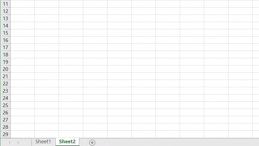
Unlike Columns, Rows and Cells, you can rename Worksheets/Tabs. By default, Worksheets/Tabs are named ‘Sheet1’, ‘Sheet2’ etc, but you can rename them and even colour code them if you wish by right-clicking on the Worksheet/Tab and selecting either ‘Rename’ or ‘Tab Color’.
Back to Top
Formulas
Excel Formulas can be used to either calculate the value of a single Cell or multiple Cells, as well as use Functions to calculate values or retrieve data.
Simple Formulas can calculate by adding, dividing, multiplying or subtracting values from other Cells. To add, you use the + symbol, to divide you use the / symbol, to multiply you use the * symbol and for subtracting you use the – symbol. For example, if you wanted to add together the values of three Cells to work out the total value, you could do this:
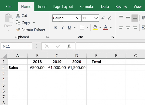
=B2+C2+D2
Here, you would select the first Cell and type the + symbol, then select the second Cell and type the + symbol again, and finally select the third Cell to create a Formula that adds together all three Cells and calculates their total value. This is not a problem if you are working with a handful of Cells, but if you’re dealing with a lot of them, it is much easier to use the SUM Function and highlight the Cells to achieve the same calculation of adding them all together, like this:
=SUM(B2:D2)
Using the SUM function to create a Formula can be a real timesaver when you’re working with a lot of data. In the example above, it shows how you can highlight multiple Cells in a Row; this also works if you need to highlight multiple Cells in a Column.
If you need to bring together data from multiple sources or from different parts of your spreadsheet, you can use Functions like a VLOOKUP, a SUMIF or a COUNTIF to retrieve certain information and/or give you an overall picture of the data you have.
Back to Top
VLOOKUP
For example, imagine you own a restaurant and you’ve got a long list of table reservations. The list contains customer contact details, party size, date the table is booked for and allergy/dietary requirements. However, you’ve forgotten to ask what time they will be arriving! Luckily, you’ve got email addresses for all of the customers, so one of your colleagues sends an email to each of them and makes another list that just has the customers’ email addresses and time of arrival. You can then quickly retrieve the times from your colleague’s list and store them alongside the correct customer in your original list by using a VLOOKUP, like this:
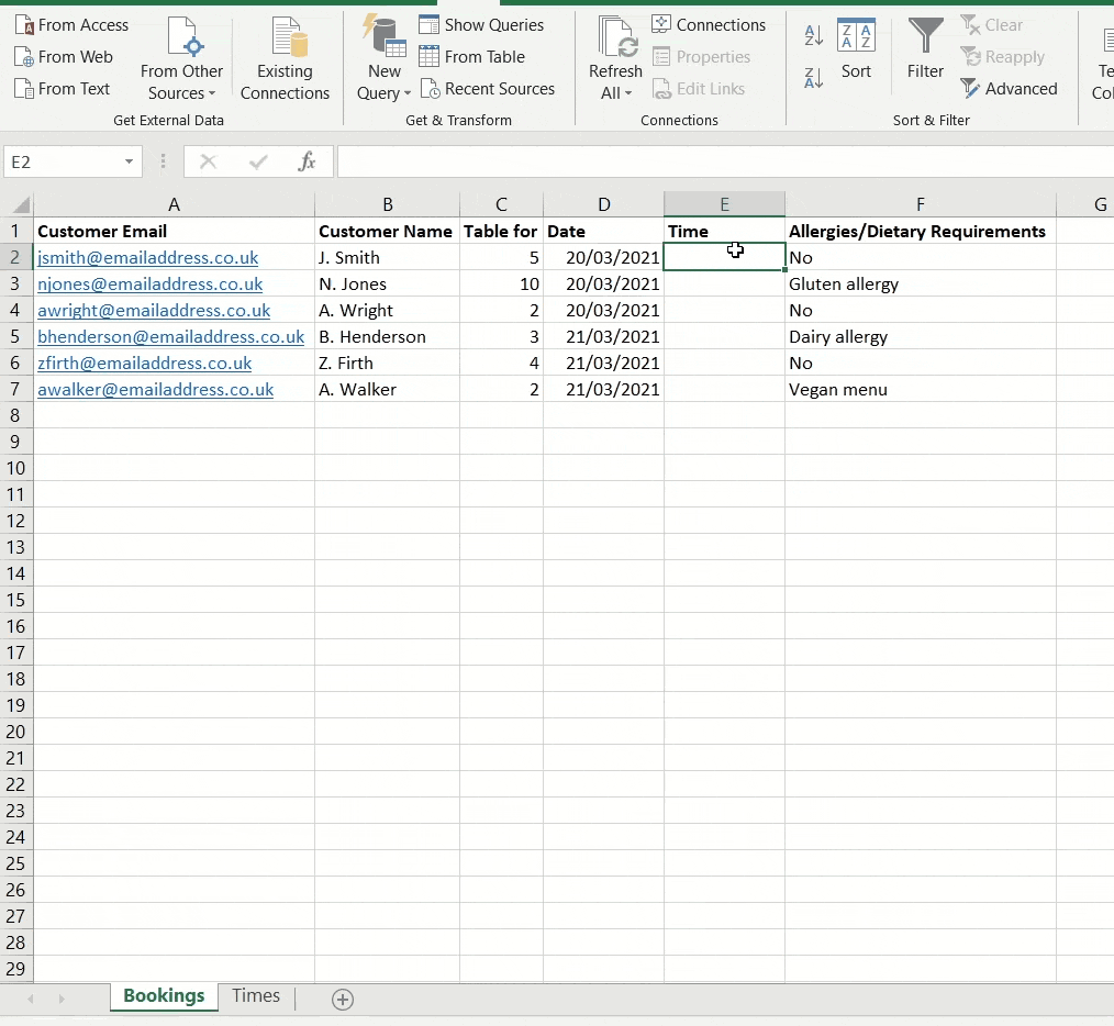
=VLOOKUP(A2,Times!A:B,2,FALSE)
So, what is this VLOOKUP doing? First, you have to ensure that there is a common identifier in both your lists. The common identifier must be identical in each list – in this case the common identifier is customer email addresses. The Column containing the common identifier needs to be located to the left of the data you want to retrieve.
So, we start off by writing =VLOOKUP( then select the ‘lookup_value’, which in this example will be the first email address in Cell A2, then type in a comma.
Your Formula should now look like this: =VLOOKUP(A2,
Next, you’ll need to go to the Worksheet/Tab that contains the other list (in this example, the Worksheet/Tab has been named ‘Times’) and select the ‘table_array’, which means highlighting the range of Columns starting with the Column containing the ‘lookup_value’ and continuing until you reach the Column containing the data you want to retrieve, then type in a comma. So for this example, in the ‘Times’ Worksheet/Tab, we’re selecting Columns A and B, Column A contains the ‘lookup_value’ and Column B contains the table reservation times.
Your Formula should now look like this: =VLOOKUP(A2,Times!A:B,
We’re almost finished…
Next, we need to type in the ‘col_index_num’ which just needs you to count along from the first Column in your ‘table_array’ until you get to the Column which contains the data you want to retrieve. In this example, the data we want is in the second Column in the ‘table_array’ so we just need to type 2, then a comma.
Your Formula should now look like this: =VLOOKUP(A2,Times!A:B,2,
Finally, we need to choose a ‘range_lookup’. There are two choices here: ‘TRUE’ or ‘FALSE’. ‘FALSE’ is usually the best option to choose as it means that the VLOOKUP will find the exact match to the ‘lookup_value’ you selected at the beginning of this Formula. Once you’ve selected or typed in ‘FALSE’, you can just hit Enter on your keyboard and the VLOOKUP will use the details you’ve selected and input, then go and find the data you wanted. Once it finds this, it’ll place it in your original Bookings list.
Your finished Formula should now look like this: =VLOOKUP(A2,Times!A:B,2,FALSE)
As shown in the image above, once you’ve written this VLOOKUP you can locate the Fill Handle in the bottom right corner of the Cell (in this example, the Cell is E2) and drag the handle down to the bottom of your list. The VLOOKUP Formula will change for each Cell and retrieve relevant data based on each customer email address.
This is just one example of how to use a VLOOKUP. There are many other applications and they don’t all need to be focused on email addresses. You might want to use order/invoice reference numbers or customer usernames instead.
Back to Top
SUMIF
There may come a time when you need to add up values in a particular Column, Row or specific Cells based on certain criteria. For example, imagine you own a restaurant and you have a list of all your bookings, the list contains customer contact details, party size, date and time the table is booked for and allergy/dietary requirements. Now, if you wanted to add up how many people are going to attend your restaurant on a certain day, you can use a SUMIF like this:
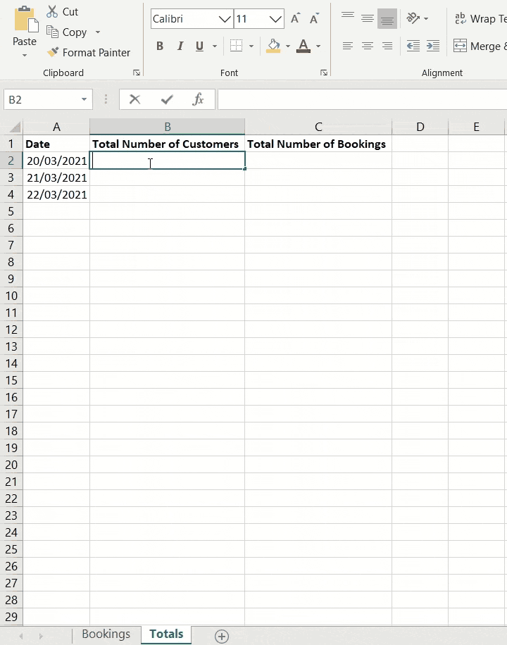
=SUMIF(Bookings!D:D,Totals!A2,Bookings!C:C)
Let’s look at what this SUMIF is doing. We’re trying to add up the total number of customers arriving on certain days and the SUMIF allows us to do that. First, we need to write =SUMIF( in Cell B2, just under the appropriate heading ‘Total Number of Customers’, then go to the Worksheet/Tab that contains the list of all your bookings (in this example, the Worksheet/Tab has been named ‘Bookings’) and select the ‘range’, which means highlighting a single Column, a single Row, or a specific range of Cells that contains the information you want to search and match, then type a comma. So, for this example, in the ‘Bookings’ Worksheet/Tab we’re selecting Column D as it contains all the date information for each booking.
Your Formula should now look like this: =SUMIF(Bookings!D:D,
Next you’ll select the ‘criteria’, which in this example will be the first date in Cell A2 of the ‘Totals’ Worksheet/Tab, then type a comma.
Your Formula should now look like this: =SUMIF(Bookings!D:D,Totals!A2,
Finally, we need to go to the Worksheet/Tab that contains the list of all your bookings and select the ‘sum_range’, which means highlighting a single Column, a single Row, or a specific range of Cells containing numeric data that you want to add up and calculate a total value for. So for this example, in the ‘Bookings’ Worksheet/Tab we’re selecting Column C as it contains all the party size information for each booking. Once you’ve selected the ‘sum_range’ you can just hit Enter on your keyboard. The SUMIF will then use the details you’ve selected and input to go and find the data you wanted and calculate the total value.
Your finished Formula should now look like this: =SUMIF(Bookings!D:D,Totals!A2,Bookings!C:C)
As shown in the image above, once you’ve written this SUMIF you can locate the Fill Handle in the bottom right corner of the Cell (in this example, the Cell is B2) and drag the handle down to the bottom of your list. The SUMIF Formula will change for each Cell and calculate the total number of customers due to arrive for each date.
Back to Top
COUNTIF
You may find that you need to count how many times a certain value appears in a Column, Row or specific Cells. For example, imagine you own a restaurant and you have a list of all your bookings. Each row of the list relates to a booking and contains customer contact details, party size, date and time the table is booked for, and allergy/dietary requirements. Now, if you wanted to count how many bookings have been made for certain days you can use a COUNTIF like this:
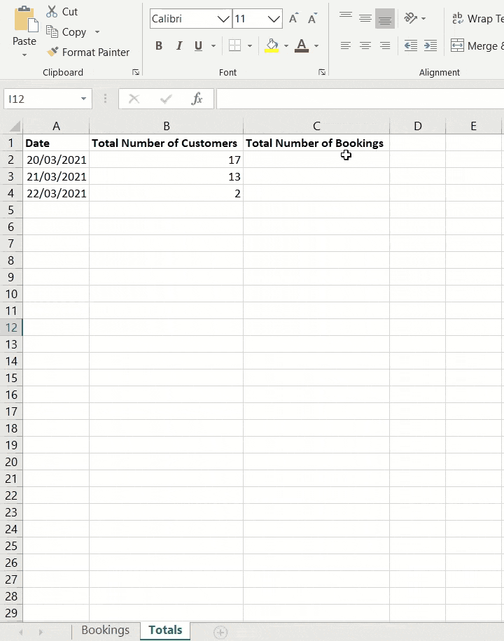
=COUNTIF(Bookings!D:D,Totals!A2)
Let’s look at what this COUNTIF is doing. We’re trying to count how many bookings have been made for certain days and the COUNTIF will work that out for us. First, we need to write =COUNTIF( in Cell C2, under the heading ‘Total Number of Bookings’, then go to the Worksheet/Tab that contains the list of all your bookings (in this example, the Worksheet/Tab has been named ‘Bookings’) and select the ‘range’, which means highlighting a single Column, a single Row, or a specific range of Cells that contains information you want to search and match, then type a comma.
So, for this example, in the ‘Bookings’ Worksheet/Tab we’re selecting Column D as it contains all the date information for each booking.
Your Formula should now look like this: =COUNTIF(Bookings!D:D,
Finally, you’ll select the ‘criteria’ which in this example will be the first date in Cell A2 of the ‘Totals’ Worksheet/Tab. Once you’ve selected the ‘criteria’ you can just hit Enter on your keyboard and the COUNTIF will use the details you’ve selected and input to go and find the data you wanted and count how many times the data can be found.
Your finished Formula should now look like this: =COUNTIF(Bookings!D:D,Totals!A2)
As shown in the image above, once you’ve written this COUNTIF you can locate the Fill Handle in the bottom right corner of the Cell (in this example, the Cell is C2) and drag the handle down to the bottom of your list. The COUNTIF Formula will then change for each Cell and count the total number of bookings due to arrive for each date.
Back to Top
Charts and Graphs
Excel Charts and Graphs can be really useful to visualise data and give a clearer picture of what the data can tell you.
Looking at numerous Columns and Rows full of various information can be a bit hard on your eyes and in some cases it just looks meaningless. This is where Charts and Graphs can help by showing the data in a different way, which may result in you spotting some sort of trend or pattern.
To create a Chart or Graph in Excel you’ll first need some data. Following on from the examples above, we have some data relating to restaurant customer numbers and booking numbers for certain dates.
Excel is smart, so if you highlight cells which contain things like a series of dates, headings and data you can go to the ‘Insert’ section, which is located towards the top-left of your screen, and select ‘Recommended Charts’. This will then present you with some appropriate charts and graphs, like so:
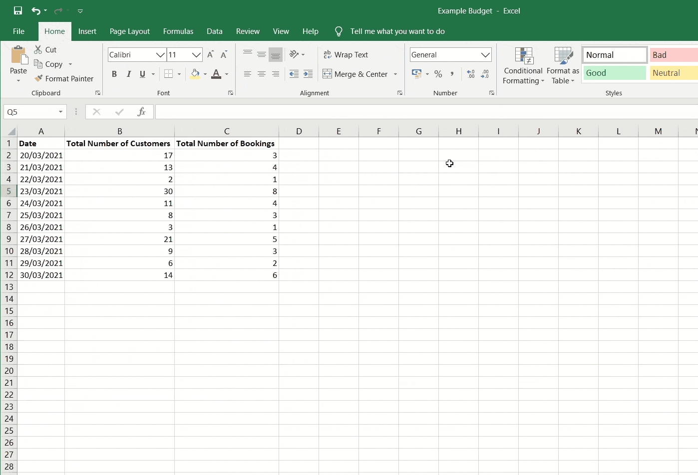
Before we end, let’s give you another practical example of how Excel could be used based on what we’ve already covered.
Back to Top
Using Excel to Create a Budget Sheet
We’ve mentioned budgets earlier in the guide, but now let’s look at how Excel can be used to create a budget. We’ll start by opening a blank workbook in Excel and then begin writing some appropriate headings (e.g. Outgoings, Name, Category, Months).

A first tip to make a note of is if you’re entering information like dates or months into Excel, it is smart enough to recognise what you’re trying to do. If you locate the Fill Handle in the bottom right corner of the Cell that you entered the first date/month in and drag up/down/sideways as demonstrated below, it will automatically input the next dates/months into the Cells you drag the handle over.
For example, here we’ve entered ‘Jan’ into Cell D2 and then dragged the Fill Handle across to the right all the way to Cell O2. Once we’ve finished dragging the handle across, the month names appear in the Cells.
Continue to enter appropriate headings both across Columns and Rows, then enter the names and categories for each item of your budget into the relevant Cells. For example, imagine you own a restaurant and you’re trying to create a budget which details outgoing spend and incoming revenue. The names and categories for each budget item might look something like this:
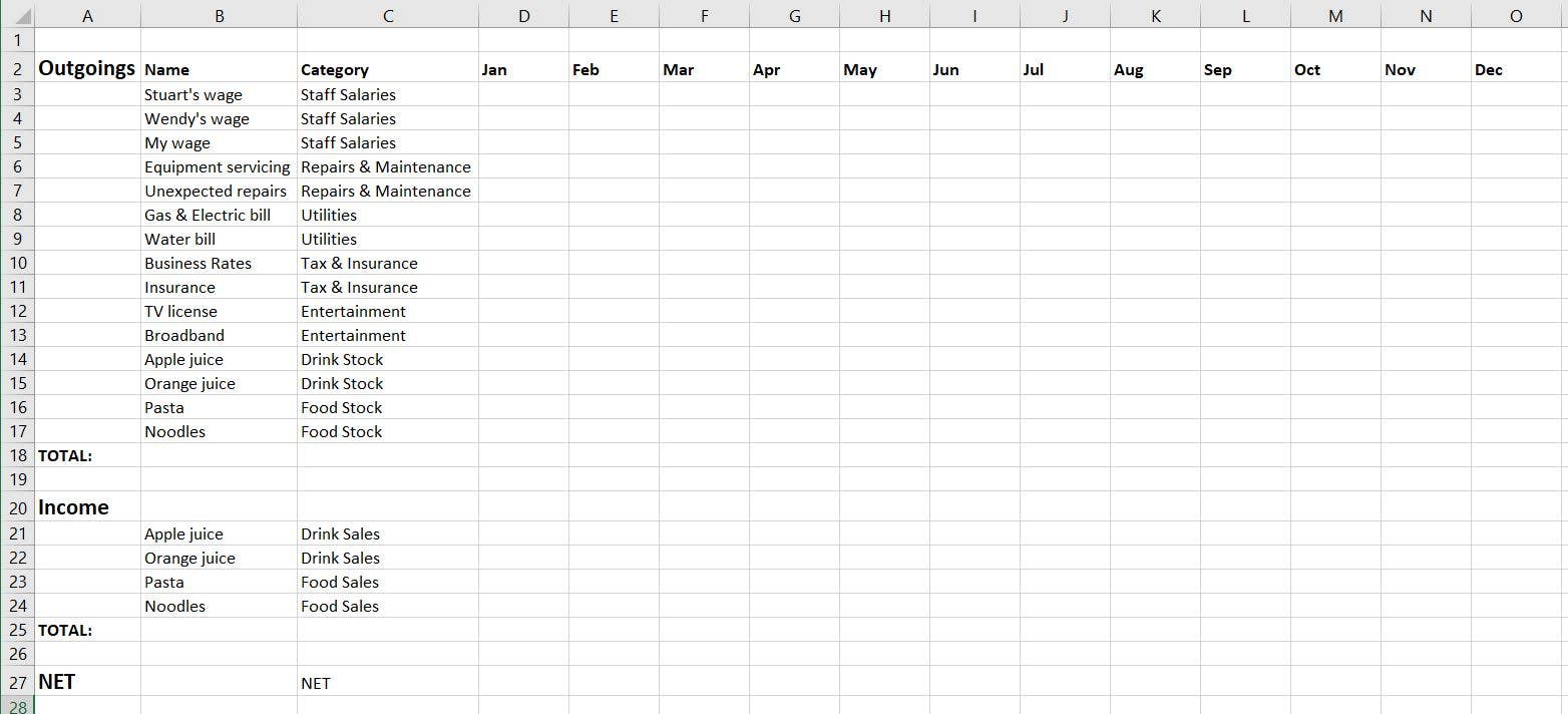
This details outgoings such as staff salaries, repair costs, utility bills and food/drink stock, as well as listing income such as food/drink sales.
Next, we can start entering financial values for each budget item and month. These figures may be based on previous accounts you’ve kept or they may be based on your best guess and available information. Now that you’ve entered those figures, it is best to format them so they are presented as currency.
To do this, simply highlight all the Cells you’ll be using to store or calculate financial values and then right-click. A menu of options will appear and here you need to select ‘Format Cells’. Another set of options will then appear and in here you just need to select ‘Currency’. If the ‘Symbol’ is not set to the currency you need, you can click on it and choose from a list of different currencies. Finally if you want to display negative numbers differently, there are a few options available.
Once you’re happy with your selections, click OK and the numeric values in the Cells you highlighted will change to present as currency, like so:
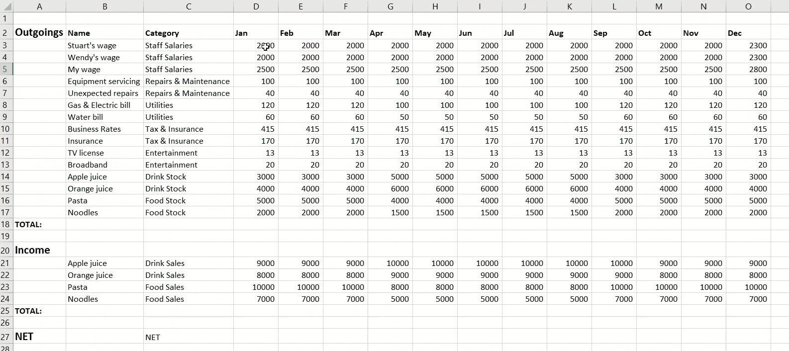
Now that you’ve entered and formatted the financial details for all your budget items, you can use the SUM Function to create a Formula that will calculate the monthly total for all your outgoings, like so:
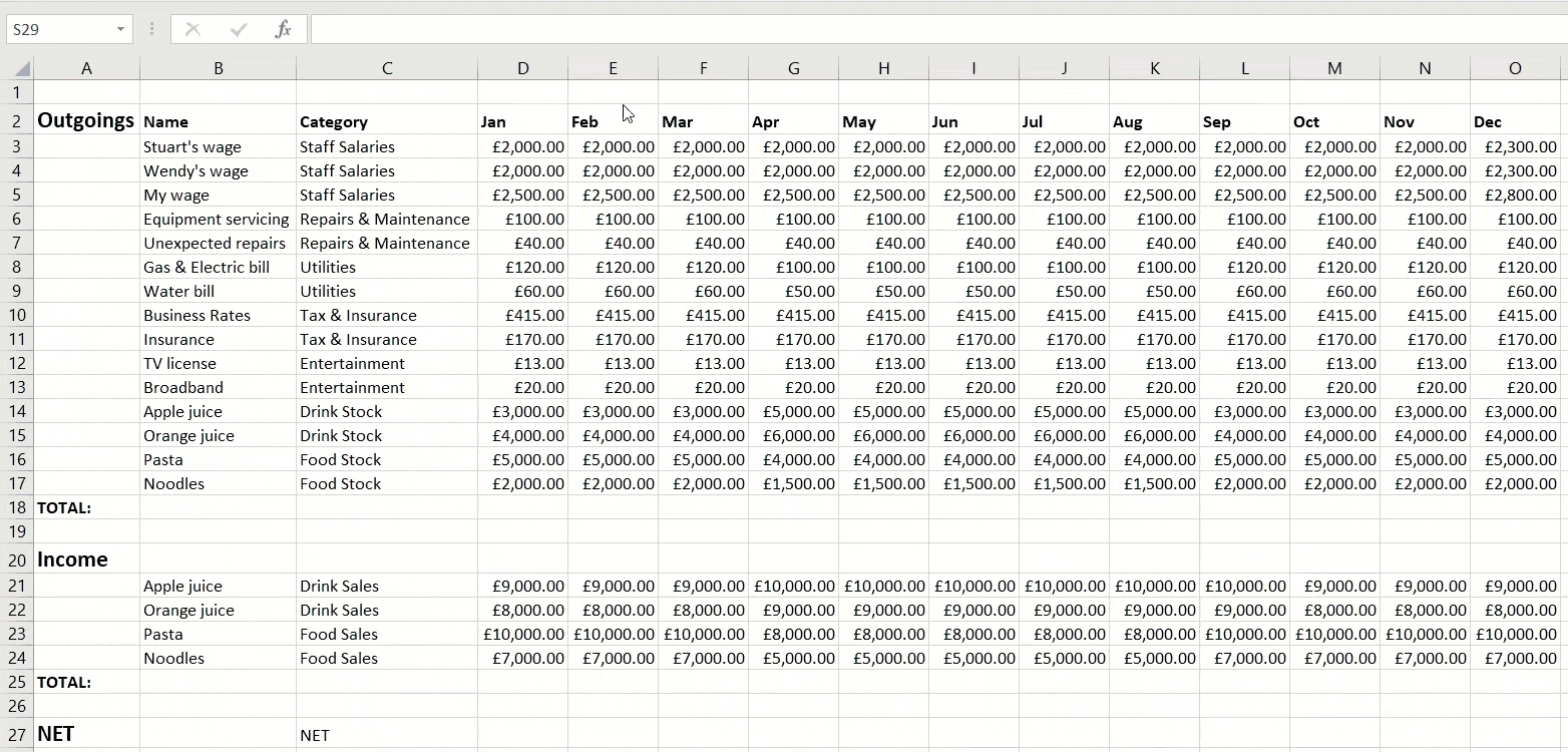
Here you can see that instead of selecting a whole Column, the SUM is being calculated for certain Cells, and then by using the Fill Handle the Formula is repeated and used to work out the total outgoing for each month. You can then create a similar calculation to work out the total income for each month.
Finally, we can work out the Net amount for each month by writing a simple Formula to subtract the monthly outgoings total from the monthly income total, like this:
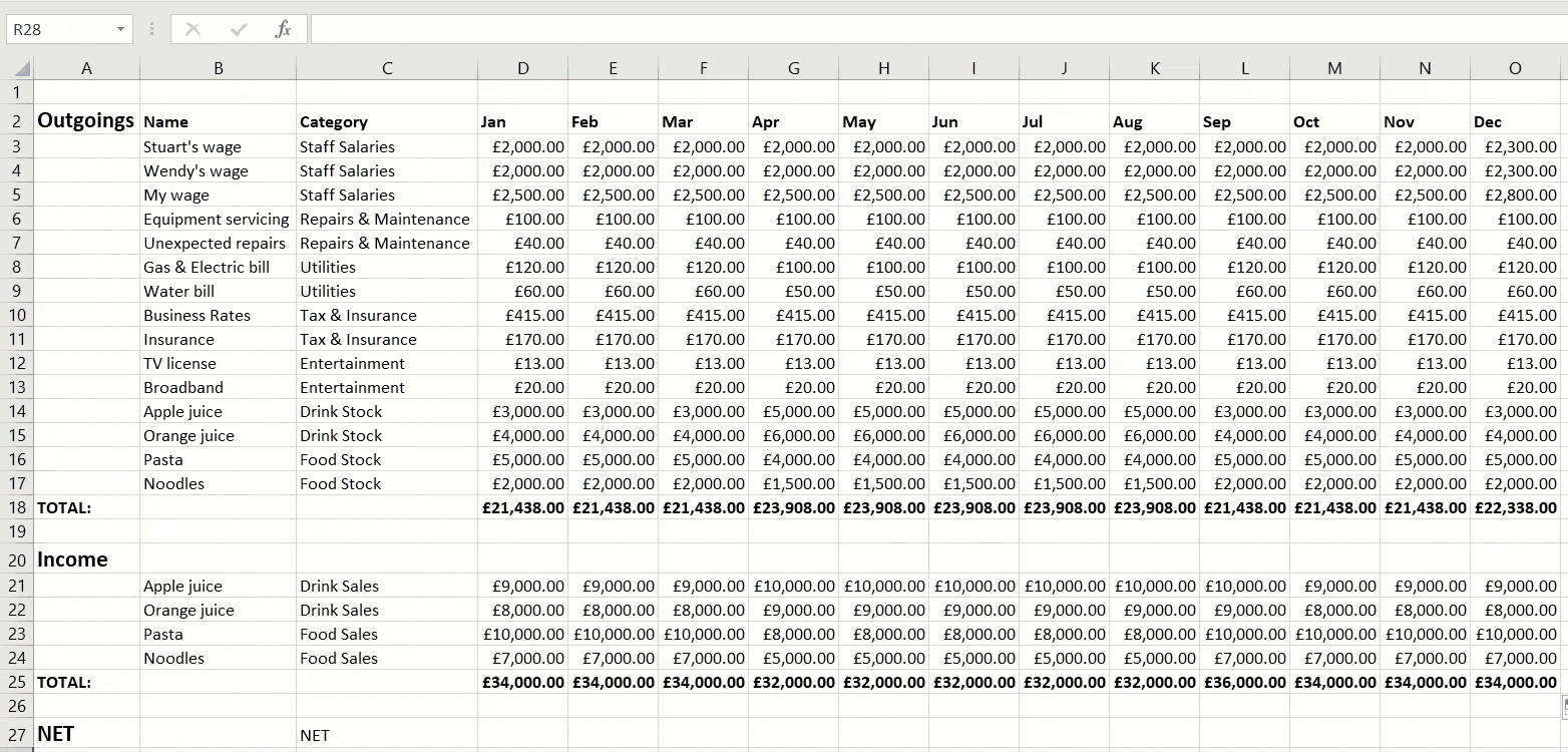
And there you have it – a simple budget using a combination of SUM and basic Formulas. You could take this further and apply what you’ve learned about SUMIF to work out which category of your budget costs the most in December and which category of your budget generates the most income in December. You could even make a Chart or Graph of your findings. Give it a try and good luck.
Back to Top
What’s next?
Once you fully understand these Excel basics, the next step would be to grow your Excel knowledge further by researching Pivot Tables, Data Validation and Functions like IF, SUMIFS and COUNTIFS. You can find all sorts of guides online by searching on Google or YouTube. Watch this space too, as we’re always releasing new guides on all sorts of topics to help you with your personal and professional growth.
Further Resources:
- Writing A Professional Development Plan – Example & Template
- Writing a Job Description: Free Template
- How to Upskill Yourself
- Microsoft Excel and Google Sheets Training for Beginners


- Meet our Expert: Stephanie Jones
- What is Excel?
- Pros & Cons of Excel in Data Analysis
- Most important functions of Excel for data analysis
- Data Jobs that Use Excel
- Can You Learn Excel at a Data Analytics Bootcamp?
- The Future of Excel
Table of Contents

Since 1987, Microsoft Excel has been used in virtually every office by employees with various job titles. But how is Excel used in data analysis today and can it be learned at a bootcamp? Thinkful Data Analytics Instructor Stephanie Jones explains the pros and cons of using Excel for data analysis, the top Excel functions that every data analyst needs to know, and Stephanie’s favorite free resources (and datasets) to start learning Excel!
Meet our Expert: Stephanie Jones
-
Stephanie received a BS in Math from the University of Denver and a Master’s in Statistics from the University of South Carolina.
-
Stephanie has plenty of real-world experience in data too, working as a Revenue and Data Science Analyst and as a consultant for a natural language processing company that focused on AI solutions. Stephanie also helped develop a statistics curriculum for the University of South Carolina!
-
Her passion for teaching adult career-changers led Stephanie to become an instructor at Thinkful, where she loves the one-on-one aspect of the program and giving personalized instruction: “I was excited about the opportunity to jump into the bootcamp world because it is an adult learning space that addresses all learning types,” says Stephanie, “We support those who have test anxiety or have life situations that prevent them from turning in a homework assignment everyday. I love that and that’s why I chose Thinkful.”
What is Excel?
Excel is a spreadsheet software. Excel is a convenient go-to software that is both comprehensible and familiar, and a key part of Excel is how it can be used for ad hoc analysis. Many people are familiar with Excel and that level of comfort is where much of its power stems from.
How do Data Analysts use Excel?
Data analysts use Excel in much the same way that you might use the calculator app on your iPhone. When you aren’t sure what is going on with a dataset, putting it into Excel can bring clarity to the project.
You don’t have to be a Data Analyst by title to start using Excel, though. If you can type and hit enter, then you can start using Excel. That’s the beauty of it – you can self-study and continue to learn. And with Thinkful, you have someone like me who will help you when you are stuck!
What types of data can be entered into an Excel spreadsheet?
Everyone thinks of financial data with Excel, but it can apply to any industry data – I’ve even worked on FDA approval cases and human resources datasets! All types of data are appropriate!
The only exception would be the size of the datasets. Small to medium-size datasets are best for Excel. If a dataset becomes too large, it’s cumbersome in Excel. Many times, data analysts will take a look at the underlying data using Excel before they use a heavier application like Python or SQL.
Give us an example of a problem that a data analyst could solve with Excel!
A scheduling manager could use Excel to record their employee’s schedules. When Joe, your employee, complains about being scheduled on Friday afternoons, you can sit down with Joe and breakdown the data to see if he was being disproportionately scheduled. Using the dataset, you can offer him a straight answer with no emotion attached. That’s the best part about data analytics! You receive a final answer at the end that is logical and impossible to deny.
Pros & Cons of Excel in Data Analysis
What are the pros and cons of using Excel for data analysis?
Excel is powerful because it’s quick and easy to use, but the downside is that it isn’t scalable. As data sizes become larger, we hit limits in our notebook and time limits on our computer. Excel also lacks the ability to automate processes.
Are there alternatives to Excel?
Google Sheets is a free alternative to Excel. The collaborative aspect in Google Sheets is great, but it also makes it harder to protect your data from other parts of the company. It is awesome software but Google Sheets isn’t quite as advanced as Excel is and I doubt they will ever catch up. Excel is continuously improving and expanding.
As a Business Analyst, I am typically sharing data with Tableau or Excel. If I needed someone on my team to change something, though, I would never share with Tableau. I would only be comfortable sharing with Excel, because I know my team will be comfortable working with it.
Most important functions of Excel for data analysis
Any function that can break down data is useful for data analysts.We often hear about the Excel VLOOKUP function, which has actually been replaced by XLOOKUP within the newest version of Excel. At Thinkful, we teach students about all three of those important Excel functions, plus Index Match which is a little more difficult to master, but provides a more robust solution. Other Excel functions to break down your data include pivot tables, VLOOKUP, sorting, and filtering.
PIVOT TABLES
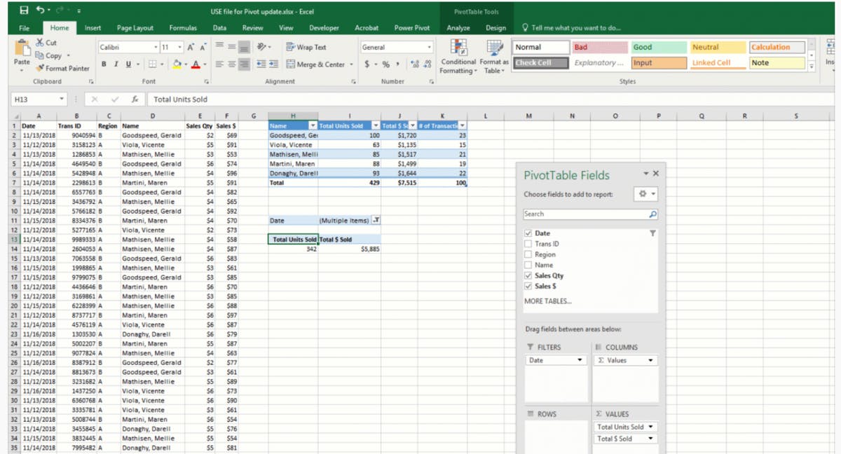
Pivot tables are a way to aggregate data to look at smaller subsets without using manual filters. Without it, you would use the manual filters on every column, check to see if they work, and then use [SUM] functions. All of that is built for you with a pivot table and pivot chart. The best part is that pivot tables are quick and easy to change. If you are in a meeting and someone wants to see 2019 instead of 2020 data, in just one click you can change the filter and all of your visualizations and pivot charts will change.
VLOOKUP
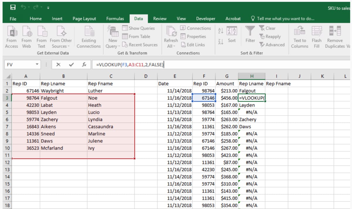
VLOOKUP is the most popular function in Excel to bring together two datasets. For instance, if you have employee numbers in one table and names in a separate table, but want to bring them together, VLOOKUP can help you do that. VLOOKUP is more accessible and logical to use when looking up a small piece of information in a dataset. If you have a larger dataset, you should use alternative methods, like XLOOKUP or Index Match. Unfortunately, Index Match is difficult for someone to learn on their own. In contrast, VLOOKUP has many detailed tutorials that can be found on the web, so you can easily teach yourself.
XLOOKUP

XLOOKUP came out in early 2020, and it was created as the solution to VLOOKUP and Index Match’s problems. XLOOKUP doesn’t work with past versions of Excel, but it is faster and much more user friendly. It will eventually be the industry standard, but because many people have old versions of Excel, VLOOKUP is still important to learn.
What is the Analysis ToolPak in Excel?

The Analysis ToolPak is a free add-on for Excel feature intended for the intermediate user. It allows users to do different statistical testing within their Excel notebook. With the Analysis ToolPak, you don’t need to know the underlying functions for standard deviation. You can run it one time, and it will put out all of those statistics at once.
Data Jobs that Use Excel
Any position with the word «analyst» at the end of it requires Excel! That includes Data Analyst, Business Analyst, Business Operations Analyst, and Reporting Analyst.
What types of projects have your Thinkful students built using Excel?
For one of our projects, students can use a dataset with housing prices for a certain neighborhood. We had just finished our Tableau section where students learned to make geographic heat maps, which is when you fill parts of the map based on frequency or quantity. One of my students wanted to learn how to use Power Maps in Excel, and together we figured out how to set that up for her.
Can You Learn Excel at a Data Analytics Bootcamp?
Since you took a traditional path into data, do you think it’s possible to learn data analytics at a bootcamp?
Bootcamps are the best way to learn data analysis. I took an expensive and long education path, but my Thinkful graduates are just as qualified as me when it comes to data analytics! At the end of the day, it’s about the result-based skills. Thinkful covers the theory enough to use it, but doesn’t force its students to memorize the formulas like I had to in a university. Students learn where to find the information and how to use the resources they will have on a job, such as the Thinkful resources on their dashboard (which they will have access to forever). I had to learn these skills on the job with my boss breathing down my neck and a coworker doing the other half of the project. It was stressful, made me feel like an imposter, and created self-doubt. In contrast, Thinkful students receive hands-on work experience throughout the bootcamp. They can be comfortable asking questions and finding solutions in a positive environment. At Thinkful, there is pressure on students to cover the material, but never to learn anything on their own. I tell my students that struggling for more than 20 minutes is not a good use of their time. They need to ask for help.
How does Thinkful’s data analytics bootcamp incorporate Excel into the curriculum?
Excel is taught throughout the entire data analytics curriculum. Any skill that we build, we build first in Excel, and then we discuss other features and ways to access data outside of Excel. We always relate it back. For example, I teach the Python section of the curriculum. As soon as we hit the Pandas section, I ask students what the Pandas dataframe looks like. The answer is, it’s a spreadsheet, which means we are right back to Excel again! Everything connects back to Excel because of the comfort-level. It doesn’t mean that it is the easiest, best, or scaleable way, but it’s a good place to start.
Can you teach yourself Excel?
Excel has official and unofficial documentation plus tutorials everywhere online. Excel and information about the software is so ubiquitous because it’s been around for so long. It’s very easy to find the answer for anything you want to do in Excel because there is always someone who has done it before and documented it.
For Excel newbies, what resources do you recommend?
-
Check out Microsoft Excel’s support page for great documentation.
-
Thinkful offers a Data Analytics prep course that our students may take before the bootcamp begins. It fully prepares the student to begin the Data Analytics immersive program. When a student doesn’t go through the free prep course work, they ask many questions the pre-work explains and that slows down the class.
-
If you’re looking for data, head to Kaggle. You can also review on people’s projects on there, too!
To practice with Excel, you need data! Where do you recommend finding sample Excel data?
-
Data.gov has a ton of datasets to play with.
-
As a statistician, I recommend Nate Silver FiveThirtyEight who publishes their datasets and some of the code. You can read the article and then review the dataset and code to run it yourself. It’s helpful if you want to learn some of the techniques they use.
-
The best place to find data is within your everyday life, such as finances, credit card statements, and work schedules. Your home and work life has familiar and comfortable data to work with, so you’ll quickly know if something in your dataset isn’t correct!
The Future of Excel
Microsoft Excel has been for a very long time. Do you see Excel retaining its importance in the future of the tech workforce?
We will always have Excel in data analysis, but it’s role is already changing. Websites like Amazon collect the data of every click, which means huge datasets. As we get bigger datasets, it won’t be feasible to apply them to Excel. Microsoft will ultimately adapt with better software to handle larger loads, but Excel will not change much. It also won’t go away because we teach it to students as early as middle school. Everyone has a basic understanding of its processes and uses it at a basic level in the workplace. Analysts will utilize Jupyter Notebook or Python code for big data projects, but the majority of the workforce will still be reading Excel spreadsheets.
Find out more and read Thinkful reviews on Course Report. This article was produced by the Course Report team in partnership with Thinkful.

We all have atleast one story of how that one time the boss / co-worker / classmate / cat ruined the carefully crafted excel spreadsheet by mucking up the formulas or disturbing the formatting. There are 3 very easy solutions to prevent this problem,
- Write an unleash_a_pack_of_wild_cats_when_someone_messes_with_the_file () macro: It is not an elegant solution, and cats are not very consistent, but it can work.
- Move to marketing department, you dont need to send excel files any more, just ppts. 😛
- Or, read this post and learn 10 awesome tips on how to boss proof your excel files.
So here is the list of 10 tips to make better excel spreadsheets. I suggest using all these tips for a perfect boss proof workbook.
Restrict The Work Area Few Columns and Rows
Not all spreadsheets have 256 columns and 65000 rows of data. So why show the entire grid when you can, say, just show the 44 rows and 23 columns in which the sales report is presented.
To restrict the work area,
- Select the first column you dont want to see (24th column) and press CTRL+SHIFT+RIGHT ARROW. Now Right click and select “Hide” option.
- Select the first row you dont want to see (45th row) and press CTRL+SHIFT+DOWN ARROW. Now right click and select “Hide” option.
Lock Formula Cells And Protect The Worksheet
Formulas are the most vulnerable part of an excel sheet. You accidentally edit something, say in payroll sparesheet, and you just gave 3200% bonus to someone in the organization. That is alright if that someone is a CEO of a bailed-out bank, but in all other cases, you end up spending a sweet afternoon trying to figure out what went wrong.

So, it is better to lock the workbook formulas and protect the worksheet so that no one accidentally erase the formulas or mess with them. To do this follow the steps in the illustration above.
You can use the same trick to lock the charts and other worksheet objects.
Freeze Panes So that Your boss Knows what she is Reading

Freeze panes is a very useful feature. It locks the important items on the top so even when you scroll down you still see them. (You can do the same for columns, thus seeing the first few column even when scrolling left).
Bonus tip: Use excel tables (new feature in Excel 2007) so that you dont need to freeze panes. Learn more.
Hide Un-necessary / Calculation Sheets
It is fairly common for excel workbooks to have tens worksheets, some with data, some with calculations, some with intermediate stuff and only one or two sheets with actual outcome (like a dashboard or a report).

There is no reason to think that all these worksheets should be visible all the time to the boss. While it makes sense to have the data and calculations visible so that someone can audit the worksheet, I am sure you dont want your boss to waster her time doing that. So here is a handy tip:
- Select all the worksheets other than the output sheets and hide them.
Hide Rows / Columns
If for some reason, hiding worksheets is not possible, you can still try hiding rows and columns. This is a very good way to prevent someone from accidentally messing a with a row of “really big and complicated formulas”.

Just select the rows / columns you want to hide and right click and select the “hide” option.
Include Cell – Comments / Help Messages
We all know bosses have a busy mind. They dont have time to remember (or know) every little thing. Heck, sometimes they dont even know what somethings are.

I suggest using cell comments and help messages to give right information / guidelines to the spreadsheet end user, like “enter your age in this cell”. They are easy to implement and totally non-intrusive.
- To include a cell comment, select the cell and press SHIFT+F2 and write the comment.
To include a cell message, select the cell, go to data validation, go to “input message” tab and type what you want.
Data Validations, Error Messages
Spreadsheets are complicated things that are carefully crafted with umpteen pre-conditions and assumptions. I am sure there is at least one excel file out there that will only work if a cat enters the input. But we are not talking about cats, the point is, it is important that right data is fed to the worksheet before the formulas (or charts or payroll macro etc.) can work. That is where data validation can help.

It is very easy to set up data validation in excel. Just select the cell and go to data validation (in Data ribbon / menu). There are several ways in which you can set up data validations,
- You can show an incell drop down box and ask users to pick from a list
- You can specify the type of data allowed (dates, times, numbers, text)
- You can specify the length of data
- You can specify the conditions on data (like between 2 numbers, less than a given date etc.)
- You can even use formulas to make your own data validations [example]
There are several examples of using data validation in this site. Go check.
Use Consistent Colors And Schemes
Anything looks better when it is consistent, even when it is internally screwed up. That same rule applies to excel workbooks as well. It will make your boss feel comfortable and relaxed to see an excel workbook with consistent colors and (simple) schemes.
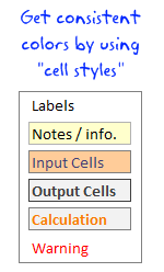
I suggest using excel cell styles to define the styles for your workbooks. This ensures consistency and you dont have to spend after hours formatting the worksheets. Read more about cell styles.
Name and Color Worksheet Tabs Appropriately
It doesnt matter if you have designed an awesome excel dashboard, your boss can be still pissed because the sheet name is “Sheet 69”. That brings us to the last and final point.

Use appropriate names (and may be tab colors) for the worksheet tabs. This makes the navigation easy and boss proof.
Learn how to color excel worksheet tabs.
Before Closing The Workbook, Select Cell A1 On The Correct Sheet
Just before you finally save the workbook and e-mail it to the boss, make sure you are on the right worksheet (ie the dashboard or the report) and selected cell A1. The ensures that when the boss opens the workbook, she sees the right tab with right information, not some calculations or formulas.
That is all, you have just learned a handful of trick to impress your boss.
Share your boss proofing tricks for excel
Got an awesome idea that has been working on your boss? Share it with us in comments. I love to hear your stories and how you are using excel to further your career.
Be awesome, Learn few more excel tricks:
We at PHD have a simple goal – “to make you awesome in excel and charting”. Here is a list of articles I recommend reading if you are new here or just wanted to be more.
- 15 fun and exciting excel tips – who say spreadsheets are boring?
- 15 Excel formulas beyond IF() and SUM()
- 15 Excel productivity tips that you dont know
- 10 things about Excel 2007 that you should know to work better
- More articles on excel productivity
Dilbert cartoon from Dilbert.com
Share this tip with your colleagues

Get FREE Excel + Power BI Tips
Simple, fun and useful emails, once per week.
Learn & be awesome.
-
70 Comments -
Ask a question or say something… -
Tagged under
cell comments, cell styles, data validation, excel 2007, freeze panes, hide, hide sheets, howtos, Learn Excel, list, list posts, lock cells, microsoft, productivity, protection, spreadsheets, tutorials, unhide sheets, using color, using excel, worksheet protection
-
Category:
Excel Howtos, Featured, Learn Excel

Welcome to Chandoo.org
Thank you so much for visiting. My aim is to make you awesome in Excel & Power BI. I do this by sharing videos, tips, examples and downloads on this website. There are more than 1,000 pages with all things Excel, Power BI, Dashboards & VBA here. Go ahead and spend few minutes to be AWESOME.
Read my story • FREE Excel tips book


Excel School made me great at work.
5/5

From simple to complex, there is a formula for every occasion. Check out the list now.

Calendars, invoices, trackers and much more. All free, fun and fantastic.

Power Query, Data model, DAX, Filters, Slicers, Conditional formats and beautiful charts. It’s all here.

Still on fence about Power BI? In this getting started guide, learn what is Power BI, how to get it and how to create your first report from scratch.
Related Tips
70 Responses to “10 Tips to Make Better and Boss-proof Excel Spreadsheets”
-
Proper print settings on each sheet helps your boss to print the reports quickly without hastling you after printing irrelevant stuff.
It is highly relevant that you print your reports once before circulating it to your boss or other people.
Knowing that what your boss actully look at in the entire report can be very usefull. You can build a good summary of what your boss wants and put that as separate tab in the form of dashbord report, so that your boss does not peep into rest of your work and start pocking you with irrelevant stuff.
You can also put that Dashboard into the email summary and not trouble your boss to open your workbook. This is ultimate boss proof tip and I have been using this for long time now.
-
Thank you Chandoo. Great checklist to follow before delivering an excel spreadsheet to someone else. Some points you mention are seemingly so simple that we might overlook them — like selecting cell#A1, but they make a difference to the impression the spreadsheet creates at the recipient’s end.
-
 Tom says:
 Dear Chandoo,
Great tricks.One trick I use (more and more) is to hide the sheet tabs and to hide the formulabar via the ‘tools’ ‘options’ and the ‘view’-tab.
Another trick is to limiting the scrolling area to hide all columms (or rows) until the end of the sheet. Select the column, press CTRL+SHIFT+RIGHT, right-click on the column and hide (also possible via VBA).
I was wondering though if ‘boss-proof’ is related to ‘excel-stupid-proof’?
Cheerio
Tom-
Arindam says:
Just wondering if the hiding formula bar really works when a recipient opens it whose «view-show-Formula Bar» is still checked…
-
T says:
It’s saved to the sheet I believe.
-
-
-
Martin says:
Absolutely agree with this post !!!
on the past months, after reading this blog, PTS’s and Debra’s Contextures, one of the things I’ve beggining to do as a best practice is to create all my spreadsheets with 3 tabs: data, summary and control, and this last one generally xlveryhidden, and sometimes the data one hidden as well.
And this restrictions are also being applied as best practice, and with a lot of benefits as you well mentioned. Furthermore, if combined with dynamic named ranges, formulae is more readable to users, and the WOW effect is often achieved when the question «How did you do that?» arises…..
Keep on the good posts !!!
Rgds,
Martin
-
Ruthie says:
Would you mind sharing an example of this technique?
-
-
Is there a way to keep the data in a seperate file rather than the same excel. This way you could keep presentation and data separate. But not sure how you would link up the two excel files
-
Pieter says:
Yes, there is a way but it is not prefered.
I used this a coulple of times, (You need to code).mail me if you need assistance with some sort
-
T says:
It entirely is possible. The problem comes though, when you share the spreadsheet.
If the recipient doesn’t have both files, or access to both, things break when the values try to refresh.
-
-
bazlina says:
ey, why is the boss a she??
-
applehead says:
haha — welcome to the future. About time.
-
-
Karthik says:
Chandoo, one more trick that we could use with the help of VBA, RT click on the View code of the particular sheet, in the properties table set the Visible status to 2-xlveryhidden, this ensures the sheet name does not show up even when the BOSS tries to unhide the sheet from the sheet >> unhide option. Dont forget to password protect the VBA (available under tools >> VBAProject properties.
-
Very good tips, although I have to say Chandoo, that your cats probably need to be spayed or neutered if they behave like that. =)
-
Good to see all these tips on a single «sheet», and giving the name *boss proof*, and Dilbert was a great welcome 😀
-
Peter H says:
The best way to «Boss Proof» (and «Self Proof»!!) a spreadsheet is to keep back ups. I use a macro that saves the last 3 significant versions of the spreadsheet all with a date stamp included in the file name.
-
To quickly select cell A1 on all sheet, use CTRL-Page UP or CTRL-Page down to navigate between sheets and CTRL-Home to select cell A1 (if you have frozen pane, it will select the top left cell of the section below).
-
Great list. And I follow every single item… I also use a consistent background color for input cells in every report/dashboard. And I use a little VBA to identify the user and change the report accordingly (selecting the right market, for example).
-
Tim Buckingham says:
Chandoo, Nice post. I like to use the hidden Paste Picture Link option. Keep the original report you want displayed on a hidden sheet and only show the boss the report picture. Also great to watch the confusion when boss trying to select cells is worth the effort!
-
m-b says:
I usually save as PDF if there’s no interactivity in the report. That way nothing can go wrong 🙂
-
Janet says:
PDFs work a dream for me too and saves the boss’s EA from telling me all the time that she can’t print my work!!
-
-
@All.. thanks a ton for sharing your ideas. I am thinking of writing a part 2 of this post explaining some of your ideas in detail.
@Bazlina … I will make sure the boss is a HE in the next post 🙂
-
Hui… says:
«10 Tips to Make Better and Boss-proof Excel Spreadsheets»…
Unless of course your Boss reads PHD ! -
Debra McLaren says:
Great article with one glaring error.
If (like me) the majority of your spreadsheet errors are *caused* by cats, adding more cats is just going to increase the problem.
-
@Hui you always have a boss, even if you are boss. If you dont have a boss, then may be a cat or even a dog.
@Debra: hmm… Are you sure the cats are not after the mouse? Go learn some keyboard shortcuts.. now 😛
-
Paul Grenier says:
Great Web Site. I’ve done almost all the above in trying to build my application and it’s taken me hours and hours reading my «dummies » book. Thank you for all this information.
Is there a formula I can use that will automatically return to «A1» cell should an associate use the 10 page spreadsheet I have?
Is there a way to set an expiration date on my workbook so that beynd that date no one will get beyond the cover page?-
Russell Cooney says:
Paul, in all my «user facing» workbooks (those that I distribute) I create a named range called «Home» on the worksheet(s) that are most likely to be used. Then I write a little VBA that selects the Home range whenever that worksheet is activated or on other triggers depending on the context of the sheet. This is more appropriate for the dashboard tabs or summary tabs my job requires.
But I usually set this functionality up early on in the design process so I can take advantage of it as well. I will sometimes assign a keystroke to the GoHome macro.
-
-
JimmyG says:
I’m in the marketing department (aka the picture department) and have to say that the macros/Excel sheets from our controlling department are the worst! They come to me to sort out the mess!!
-
@Peter: You can try creating a table of contents and then place it on each and every sheet so that user can jump to anywhere from anywhere. Here is a tutorial to help you get started.
Also, You can prevent users from accessing the workbook after a certain date using macros. But users can certainly by pass it by disallowing macros on that workbook.
@Jimmy: Wow… (just kidding) Welcome 🙂
-
Ryan says:
I was recently given a spreadsheet to improve upon.
One of the «boss-proof» actions that the previous author had used was to use data validation instead of protecting the sheet to ward off people changing formulas.
After entering a formula or value into a cell, use data validation to only allow, in this spreadsheet, whole numbers between 9999999 to 99999999.
It’s a bit of a pain to actually correct stuff instead of just unprotecting a sheet, but for those that know how to unprotect a sheet, it’s a definite way to keep them from fooling with formulas. -
Raja Srinivas says:
Puchu,
We would love to see «Print» in your links section.
It helps us taking prints as neat as your posts 🙂 -
Paul Grenier says:
Chandoo,
I’ve emailed you a couple of times looking for avenues I need to try to put my workbook on the Internet.
I notice you use PremiumThemes for your Web Site…You must feel good about their service. Do you think PremiumThemes might be an option for me?
Paul -
Instead of :
Now Right click and select “Hide” option.Shortcut can be used : Ctrl+0 (to hide)..
-
danial says:
sir i wanted to know,how to hide cells or tab without hiding rows and columns? PLZ TELL ME
-
JunDR says:
Hi Chandoo!
Great tips! Im researching on an excel project now that you can create to «lighten» the size without sacrificing the data inside..
We usually encounter problems with the data, excel file is shared, in a network folder.. and there are 11 people that enters their own productivity in each tab.. however, there comes a time (uncertain) where some of the data they enter either gets deleted or changes value.. could this be a file size problem? are there other ways to create this file that will decrease data inconsistencies?thanks!
-
[…] Hide un-necessary rows to create clean looking workbooks (and 9 more tips) […]
-
[…] Presentation format: all spreadsheets, should be designed so that it is easy to follow the process flow and result. Almost every spreadsheet should be presentable and understandable to senior management without additional formatting or explanation. (tips: how to design boss-proof excel sheets) […]
-
[…] on Excel formatting here: How to make better excel sheets, Formatting […]
-
[…] on Excel formatting here: How to make better excel sheets, Formatting […]
-
[…] 10 Tips to make better & boss-proof spreadsheets in Excel […]
-
[…] tips: Learn how to make better Excel sheets Spread some love,It makes you awesome! […]
-
Janet says:
Save what you want the boss to see as a PDF. Absolutely foolproof and no cats hurt in the process.
-
malen says:
I really enjoyed allot of the tips on here, especially the one on comments on cells. That will come in handy on allot of our projects. I would also like to share on on my little tricks. I am constantly working on several different reports with several different systems and in doing so I am constantly running in problems and my way out of them is simply calling <a href»http://www.reportingguru.com/»> Reporting Guru </a> and telling exactly what I’m going through and they can tell me exactly how to get out.
-
The_Doctor says:
One of the things I’ve found to boss proof my worksheets are a few simple VBA scripts to automatically protect the workbook/worksheets, and direct them to the «Quick Look» dashboard page, I hide all of the raw data sheets before saving. The script looks like this:
Private Sub Workbook_Open()Sheets(«Summary»).Protect Password:=»password»
Sheets(«Labor Cost by Site»).Protect Password:=»password», AllowUsingPivotTables: =true
Sheets(«Labor Cost by month»).Protect Password:=»password»
Sheets(«Quick Look»).Protect Password:=»password»
Sheets(«Quick look»).Activate
ActiveWorkbook.Protect Password:=»password», Structure:=True, Windows:=False
End SubI also have a pivot that contains labor cost data which cannot be refreshed while the worksheet is locked.
Private Sub Worksheet_Activate()
Sheets(«labor cost by site»).Unprotect Password = «password»
Set pvttable = Worksheets(«labor cost by site»).Range(«a1»).PivotTable
pvttable.RefreshTable
Sheets(«labor cost by site»).Protect Password = «password», AllowUsingPivotTables:=True
End Sub -
ben says:
good
-
Your post are always with something creative , thanks for sharing this information , your post are worth reading and implementing 🙂 great job
-
apt says:
Hi,
I will try to learn every point slowly !
Shokran Chandoo.
-
SpreadSheetNinja says:
Best boss Proofing of sheets is useing indirect(address 😛 this prevents most smartass bossess from doing any actual changes cus the formula will be long and hard to understand for any bystanders..
Also putting the actual calculations on a different sheet can make a sheet bulletproof from bosses.. especialy if you put them in the Very hidden so when the boss learns how to unhide sheets he wont simply find them.
One thing iv also learned is that most bosses is scared of macros that gives «virus» warnings before beeing run 😛 That include the default warning from Excel…
Long formulas or work arounds is best way to go.
-
Novice says:
What’s the best way to amalgamate two existing excel spreadsheets into one?
Two teams use the same format spreadsheets with individual data split into calendar months and I want to make them one without manually entering the data.
-
Alt + D + D + N
Write a query and viola, Two sheets into one.
-
-
Isaac says:
Changing the properties of the file to read-only . (While the file is closed, right click on the file and check the read-only box.)
This allows my boss(es) to access the file — even change it — without being able to save their changes. If a boss likes his ‘new’ version, he can save it with a different file name.
But now — how to prevent the boss from deleting the file altogether? Or deleting the whole network?
-
pieter says:
Hey man.
Think you can go as easy as to make a shortcut that links to your read only document. Then the boss wont know of the root document. He can figure it out but lets face it. He is a boss and 70% if them wont know squat
-
-
Matt says:
Instead of «Hiding» rows & columns, I find «Grouping» works best as its very easy to quickly see if a worksheet has hidden rows/columns. Sometimes hiding a random row/column is not easily noticed and can create issues.
-
samantha says:
I have one xl sheet with different dates in many columns and one raw’s. I want to send this data to another xl sheets for each date. if somebody can help me will be great.
-
Mariateresa says:
Hello, I have just found out that I made a mistake in my spreadsheet: I had a column of negative numbers, but one of them was positive (while it should have been negative). Is there a formula/system to avoid this?
Thanks.
Mariateresa
-
rajan pradeep says:
Yes, data validation. Values you denote would be between -1 and -999,999,999.
-
-
Hi,
Hiding any worksheet can be unhidden and messed around easily. I change the visibility in visual basic from -xlSheetVisible to -xlSheetVeryHidden. By this, even if you right click on sheets, you will be unable to find the hidden sheets.
Cool? I think so…
-
sandeep says:
Very informative, Thanks
-
Cedric says:
Is there a way to lock cells in an already protected worksheet.
(Thus the entire worksheet is protected, then the entire office can open it as read only but only a few users have the password to edit the file)
I would like an additional password or prompt box so these few users don’t accidentally change formulas. -
Itss such as you learn my thoughts! You appear too understand
a lot abnout this, like you wrote thee e-book in it
or something. I fel that you just could do with some percent to presseure the message house a little bit,
but insatead off that, this iis wondeerful blog.
An excellent read. I’ll definitely be back. -
It is in reality a nice and helpful piece of info.
I am happy that you just shared this useful info with
us. Please keep us up to date like this. Thank
you for sharing. -
GraH says:
I laughed out loud reading the 2nd solution about moving to marketing department and making ppts.
I’ve been using «technical» sheets for a long time already and depending on the audience it is hidden or not. I’m currently in my NO VBA mindset, so the very hidden option is no longer. Using sheets names like: TechnicalCodes; ExplicitVariables;SetUp; HeavyCalc seem to work to my experience as they send along a message «Don’ t you mess-up here, you fool!». A «Read This» section or sheet however does not work!
Reading stuff on this site has helped me develop a good habit of using colors and themes to assist the end user in being well-behaved. In my book the best advise here, because it is about the user experience and not only about protection your own work.
For dashboards I get rid of tabs and scroll bars. Besides 2 exceptions, I need to come across a manager who can turn them on again without my help.
Seems that I forgot about protecting cells, sheets and workbooks altogether. Damn! -
Thanks for the informative article Chandoo, I’ve been struggling with Excel lately. It’s a powerful tool, but hard to learn for me.
-
Thanks Chandoo for sharing these excel sheet tips it helps me a lot to understand excel more.
-
Nice roundup, Chandoo! Here’s one more I thought would be relevant:
For Excel 2013+, you can hide the ribbon, as shown in this animated gif: https://gridmaster.io/tips/hide-ribbon-excel-space
This will simplify the interface, making it less likely for people to accidentally make changes. 🙂
-
KUMAR says:
THANK YOU SIR
-
constantine la says:
I’m better at Power BI thanks to you!
Leave a Reply
Rating: 5.0/5. From 6 votes.
Please wait…
10 Tips to Better Your Basic Daily Use Microsoft Excel Skills
Microsoft Excel is one of the most popular spreadsheet applications provided by Microsoft used mainly for Data Visualization and Analysis purposes. Most of you already knows very well what’s Excel used for? In this article, we will concentrate more on the importance of Microsoft Excel in daily life.
I am skipping the intro about what is Microsoft Excel. If you are not aware about Microsoft Excel and explore the options available in this awesome spreadsheet program provided by Microsoft in their Office package.

Here we are trying to introduce our readers to some interesting and creative ways to use Microsoft Excel in our daily life. But make no mistake, this is not an exhaustive list.
The applications of Microsoft Excel are plenty. We touch upon a few important ones in the coming paragraphs.
Top 10 Uses of Microsoft Excel in Improving Your Daily Life
-
Budgeting Personal Expenses
Managing daily expenses is a big head ache for most people. Without keeping track on the spending, it’s impossible to cut short your unwanted expenses and save some good money.
Agreed there are many applications which could help you to add and consolidate your expenses on a daily basis. All of them would definitely have an option to download Consolidated monthly or weekly reports as csv files which can be opened as spreadsheets in Microsoft Excel.
As I already mentioned Excel is one of the most powerful Data Visualization and Analysis tool. Using the data collected for your spending, various models can be made for predicting, analyzing and modelling future spending.
A lot of visualization options including a number of different types of graphs and charts are available in Excel for visualization purposes.
Read: 7 Things Highly Productive People Do Differently

Learning basics of Statistics and applying it to your spending data using Excel options, could help you understand any patterns in your spending, major areas in which you are spending money and also manage your investments to maximize savings.
Use any popular mobile apps for managing your daily expenses and towards the end of every month download monthly spending report as csv files into Excel in your computer. Then you can make use of various Excel analysis and visual tools for managing your expenses for long term.
-
Using Microsoft Excel in Managing Small Businesses
Big companies make use of Enterprise Software’s like SAP, Oracle etc. for mapping and integrating their businesses in one place. They are pretty expensive with a lot of inbuilt features and are created specially for the use of huge enterprises.
Let’s understand how you can use Microsoft Excel as a cheaper alternative to manage your small-scale business comprehensively using its data management features.
Excel is basically a spreadsheet with rows and columns where you can store your business data – about your sales, inventory etc. – in an organized way. Excel also has various features for presenting your data in an attractive way.
Dashboards can be created in Excel through which you can build a presentation layer on top of the data layer.
Apart from using Excel as a database for storing business data, it can also be used for doing various operations on your data.
Excel can do various mathematical operations – like summing up sales over a period, logical operations – like comparing values and statistical operations – like finding maximum, minimum, average sales for various period.
It can sort or filter your data. It can incorporate pivot tables into your data. Also visualize your data using interactive charts. Excel is thus a powerful tool which can be used for reporting and analysis purposes for small and medium scale enterprises.
Also See: Coworking Advantages: 9 Benefits of Coworking Spaces
-
Uses of Microsoft Excel in Education
Microsoft Excel can aid teachers in educating their children. Most schools have adopted computers for teaching their students. Teachers teach in smart class rooms with access to laptops and projectors. The old teaching techniques of filling class boards with tables and numbers are gone for good.
Teachers can educate children by creating tables and using various charts and graphical objects. Learning would be more effective, fun and interesting with the use of Microsoft Excel.
-
Trading Using Microsoft Excel
Trading in stock markets is a lucrative profession these days. Large number of people does it full time as well as part time to make some good money. They care more about intraday and swing trades as there are more chances of earning from them.
There are many technical analysis strategies that can be applied to past stock data for predicting future prices. Microsoft Excel is a very effective tool which could analyze large amount of data and develop patterns out of it.
Historical data of various stocks can be downloaded from stock exchange websites in csv format. With the help of Microsoft Excel various predictive models can be applied to the past data and thus predict future prices or trends of the stock to a reasonable accuracy.

Microsoft Excel can also be used for back testing various stock market tactics and measure accuracy of particular strategies.
There are various Stock analysis strategies like Exponential Moving Average Analysis, Open High Low Strategy, Gap Up/Down Strategy which cab be back tested for a large set of historical data and then successfully used for Stock prediction with the help of the analytic possibilities of Microsoft Excel.
Trading in stock markets is always a risky affair. The returns one gets is always in proportional to the risk he takes. Excel can only aid in do the calculations for your strategies. Your success is always dependent on the quality of your stock market strategies.
-
Microsoft Excel for Business Presentations
Business Analysts and Consultants make use of numbers of business data to convey strategic opinions to various stakeholders. Data visualization options of Microsoft Excel can be put to use in developing impressive business information dashboards.
Excel could be of great help for Project planning purposes. Gantt Charts and other project tracking tools can be set up in Microsoft Excel which could help in better management of projects.
Microsoft Excel is one important tool for management students as numbers speak more than words with respect to business. Excel helps in making sense out of numbers, thus forming business decisions backed by data.
Read: Reasons Why Outdoor Signage is as Important as Your Website in Business

-
Multiple Purpose Templates by Excel
Excel has inbuilt templates which can be used for a variety of purposes. Templates falling under different categories like business, personal, planners and trackers, lists, budgets, charts, calendars etc. are available as free templates in Microsoft Excel.
With the wide number of templates provided by Excel, you can create a Gantt Project planner for project management in your company, create monthly budgets, create loan calculators, inventory lists and a lot more.
Get the latest version of Microsoft Excel in your laptop or desktop and get access to the large variety of customizable templates provided by Microsoft Excel.
-
Mathematics Made Easier by Excel
Formula options offered by Microsoft Excel can be used for a number of mathematical calculations. Excel offers a variety of useful functions – mathematical, financial, logical, statistical, lookups and many more.
Excel is more efficient than calculators when you need to apply same calculations to a large list of data. For example, if you have a list of marks in 5 subjects for 1000 students. It would be a hectic task to find total, percentage and grade for all of them using a calculator.
But with Excel it takes hardly a minute – apply the required formulas for the first student and then you apply the same formula to the remaining entries just by dragging. Much convenient, is it?
Also read about the various shortcuts, tips and tricks provided by Excel that can make mathematical calculations much simpler and less time consuming.

-
Excel Macros
Excel also offers yet another amazing feature that goes by the name Excel macros. Macros are sets of instructions stored in Visual Basic that helps you automate actions and commands in Excel without you manually performing them.
Repetitive and complicated tasks can be programmed to run periodically or as per schedule with the help of Macros in Microsoft Excel.
Macros are a vast subject in Microsoft Excel. There is a lot more you can explore regarding macros. Macros can either be recorded or coded using Visual Basic.
Must See: Franchising: Pros & Cons of Buying a Franchise Business
-
Create Various Calculators Using Excel
Apart from the normal calculators to do the basic calculations, there are many calculators made for specific purposes. Interest calculator for loans, Profit calculators based on sales, mortgage payment calculators, Tax calculators, Credit card payment calculators and so on.
With Microsoft Excel, you create formula-based sheets for calculating any of the above values. With the design options in Excel, you can design a dashboard so that there is a better UI inside Excel for your calculator. Excel also has in built templates for various calculators.
-
Maintaining Contact List with Microsoft Excel
Now with everyone having smartphones, storing contact information has become much easier. But with Excel you can store a large amount of contact data permanently and securely. There are applications available in smartphones that could help you import contact data from your phone to excel files.
With the cloud options of Microsoft Office package, contact files created by you can be saved in cloud and shared over internet to anyone in any part of the world.
Excel is one of the most powerful tools offered by Microsoft. This article showcases only a glimpse of that. Explore to learn more.
Summing Up Importance of MS Excel in Daily Life
So far, we have seen few important ways in which Excel can be used for personal use. I guess all of you readers have a reasonable understanding now about the importance of Microsoft Excel in daily life.
Do explore more about Microsoft Excel, understand the inbuilt tools and make your work easier with MS Excel.