Insert or delete rows and columns
Insert and delete rows and columns to organize your worksheet better.

Note: Microsoft Excel has the following column and row limits: 16,384 columns wide by 1,048,576 rows tall.
Insert or delete a column
-
Select any cell within the column, then go to Home > Insert > Insert Sheet Columns or Delete Sheet Columns.
-
Alternatively, right-click the top of the column, and then select Insert or Delete.
Insert or delete a row
-
Select any cell within the row, then go to Home > Insert > Insert Sheet Rows or Delete Sheet Rows.
-
Alternatively, right-click the row number, and then select Insert or Delete.
Formatting options
When you select a row or column that has formatting applied, that formatting will be transferred to a new row or column that you insert. If you don’t want the formatting to be applied, you can select the Insert Options button after you insert, and choose from one of the options as follows:
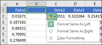
If the Insert Options button isn’t visible, then go to File > Options > Advanced > in the Cut, copy and paste group, check the Show Insert Options buttons option.
Insert rows
To insert a single row: Right-click the whole row above which you want to insert the new row, and then select Insert Rows.
To insert multiple rows: Select the same number of rows above which you want to add new ones. Right-click the selection, and then select Insert Rows.
Insert columns
To insert a single column: Right-click the whole column to the right of where you want to add the new column, and then select Insert Columns.
To insert multiple columns: Select the same number of columns to the right of where you want to add new ones. Right-click the selection, and then select Insert Columns.
Delete cells, rows, or columns
If you don’t need any of the existing cells, rows or columns, here’s how to delete them:
-
Select the cells, rows, or columns that you want to delete.
-
Right-click, and then select the appropriate delete option, for example, Delete Cells & Shift Up, Delete Cells & Shift Left, Delete Rows, or Delete Columns.
When you delete rows or columns, other rows or columns automatically shift up or to the left.
Tip: If you change your mind right after you deleted a cell, row, or column, just press Ctrl+Z to restore it.
Insert cells
To insert a single cell:
-
Right-click the cell above which you want to insert a new cell.
-
Select Insert, and then select Cells & Shift Down.
To insert multiple cells:
-
Select the same number of cells above which you want to add the new ones.
-
Right-click the selection, and then select Insert > Cells & Shift Down.
Need more help?
You can always ask an expert in the Excel Tech Community or get support in the Answers community.
See Also
Basic tasks in Excel
Overview of formulas in Excel
Need more help?
Want more options?
Explore subscription benefits, browse training courses, learn how to secure your device, and more.
Communities help you ask and answer questions, give feedback, and hear from experts with rich knowledge.
Содержание
- Процесс удаления строк
- Способ 1: одиночное удаление через контекстное меню
- Способ 2: одиночное удаление с помощью инструментов на ленте
- Способ 3: групповое удаление
- Способ 4: удаление пустых элементов
- Способ 5: использование сортировки
- Способ 6: использование фильтрации
- Способ 7: условное форматирование
- Вопросы и ответы

Во время работы с программой Excel часто приходится прибегать к процедуре удаления строк. Этот процесс может быть, как единичным, так и групповым, в зависимости от поставленных задач. Особый интерес в этом плане представляет удаление по условию. Давайте рассмотрим различные варианты данной процедуры.
Процесс удаления строк
Удаление строчек можно произвести совершенно разными способами. Выбор конкретного решения зависит от того, какие задачи ставит перед собой пользователь. Рассмотрим различные варианты, начиная от простейших и заканчивая относительно сложными методами.
Способ 1: одиночное удаление через контекстное меню
Наиболее простой способ удаления строчек – это одиночный вариант данной процедуры. Выполнить его можно, воспользовавшись контекстным меню.
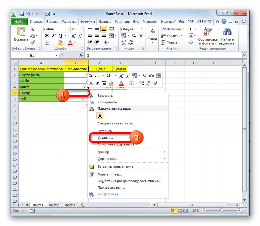
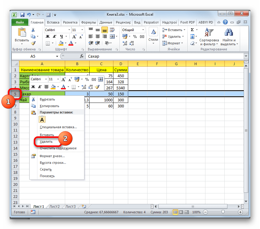
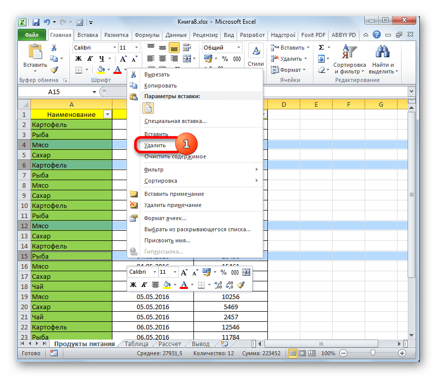
- Кликаем правой кнопкой мыши по любой из ячеек той строки, которую нужно удалить. В появившемся контекстном меню выбираем пункт «Удалить…».
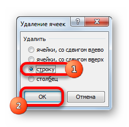
- Открывается небольшое окошко, в котором нужно указать, что именно нужно удалить. Переставляем переключатель в позицию «Строку».

После этого указанный элемент будет удален.
Также можно кликнуть левой кнопкой мыши по номеру строчки на вертикальной панели координат. Далее следует щелкнуть по выделению правой кнопкой мышки. В активировавшемся меню требуется выбрать пункт «Удалить».

В этом случае процедура удаления проходит сразу и не нужно производить дополнительные действия в окне выбора объекта обработки.
Способ 2: одиночное удаление с помощью инструментов на ленте
Кроме того, эту процедуру можно выполнить с помощью инструментов на ленте, которые размещены во вкладке «Главная».
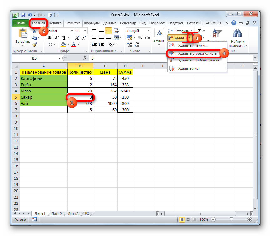
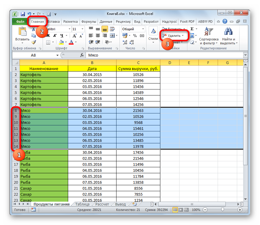
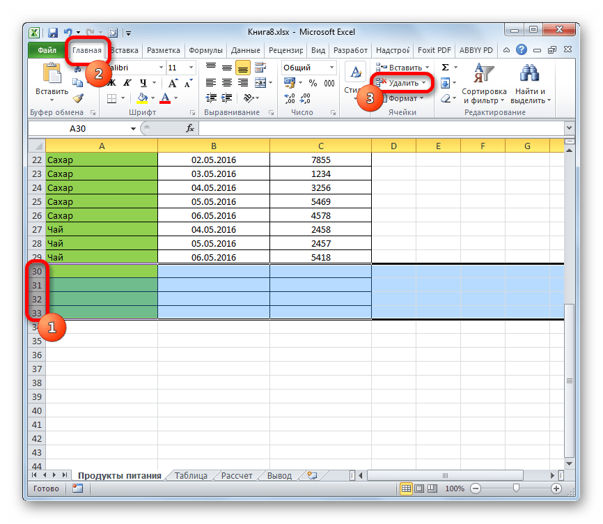
- Производим выделение в любом месте строчки, которую требуется убрать. Переходим во вкладку «Главная». Кликаем по пиктограмме в виде небольшого треугольника, которая расположена справа от значка «Удалить» в блоке инструментов «Ячейки». Выпадает список, в котором нужно выбрать пункт «Удалить строки с листа».
- Строчка будет тут же удалена.
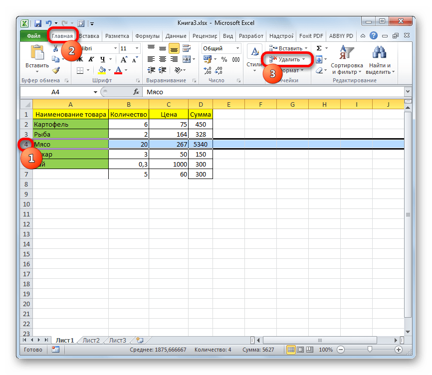
Также можно выделить строку в целом, щелкнув левой кнопки мыши по её номеру на вертикальной панели координат. После этого, находясь во вкладке «Главная», жмем на значок «Удалить», размещенный в блоке инструментов «Ячейки».
Способ 3: групповое удаление
Для выполнения группового удаления строчек, прежде всего, нужно произвести выделение необходимых элементов.
- Для того, чтобы удалить несколько рядом расположенных строчек, можно выделить смежные ячейки данных строк, находящиеся в одном столбце. Для этого зажимаем левую кнопку мыши и курсором проводим по этим элементам.


Если диапазон большой, то можно выделить самую верхнюю ячейку, щелкнув по ней левой кнопкой мыши. Затем зажать клавишу Shift и кликнуть по самой нижней ячейке того диапазона, который нужно удалить. Выделены будут все элементы, находящиеся между ними.
В случае, если нужно удалить строчные диапазоны, которые расположены в отдалении друг от друга, то для их выделения следует кликнуть по одной из ячеек, находящихся в них, левой кнопкой мыши с одновременно зажатой клавишей Ctrl. Все выбранные элементы будут отмечены.
- Чтобы провести непосредственную процедуру удаления строчек вызываем контекстное меню или же переходим к инструментам на ленте, а далее следуем тем рекомендациям, которые были даны во время описания первого и второго способа данного руководства.

Выделить нужные элементы можно также через вертикальную панель координат. В этом случае будут выделяться не отдельные ячейки, а строчки полностью.
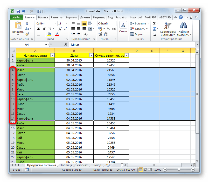
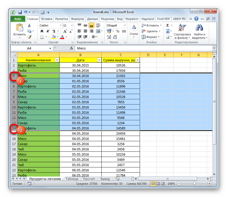
- Для того, чтобы выделить смежную группу строк, зажимаем левую кнопку мыши и проводим курсором по вертикальной панели координат от верхнего строчного элемента, который нужно удалить, к нижнему.
Можно также воспользоваться и вариантом с использованием клавиши Shift. Кликаем левой кнопкой мышки по первому номеру строки диапазона, который следует удалить. Затем зажимаем клавишу Shift и выполняем щелчок по последнему номеру указанной области. Весь диапазон строчек, лежащий между этими номерами, будет выделен.
Если удаляемые строки разбросаны по всему листу и не граничат друг с другом, то в таком случае, нужно щелкнуть левой кнопкой мыши по всем номерам этих строчек на панели координат с зажатой клавишей Ctrl.
- Для того, чтобы убрать выбранные строки, щелкаем по любому выделению правой кнопкой мыши. В контекстном меню останавливаемся на пункте «Удалить».

Операция удаления всех выбранных элементов будет произведена.
Урок: Как выполнить выделение в Excel
Способ 4: удаление пустых элементов
Иногда в таблице могут встречаться пустые строчки, данные из которых были ранее удалены. Такие элементы лучше убрать с листа вовсе. Если они расположены рядом друг с другом, то вполне можно воспользоваться одним из способов, который был описан выше. Но что делать, если пустых строк много и они разбросаны по всему пространству большой таблицы? Ведь процедура их поиска и удаления может занять значительное время. Для ускорения решения данной задачи можно применить нижеописанный алгоритм.
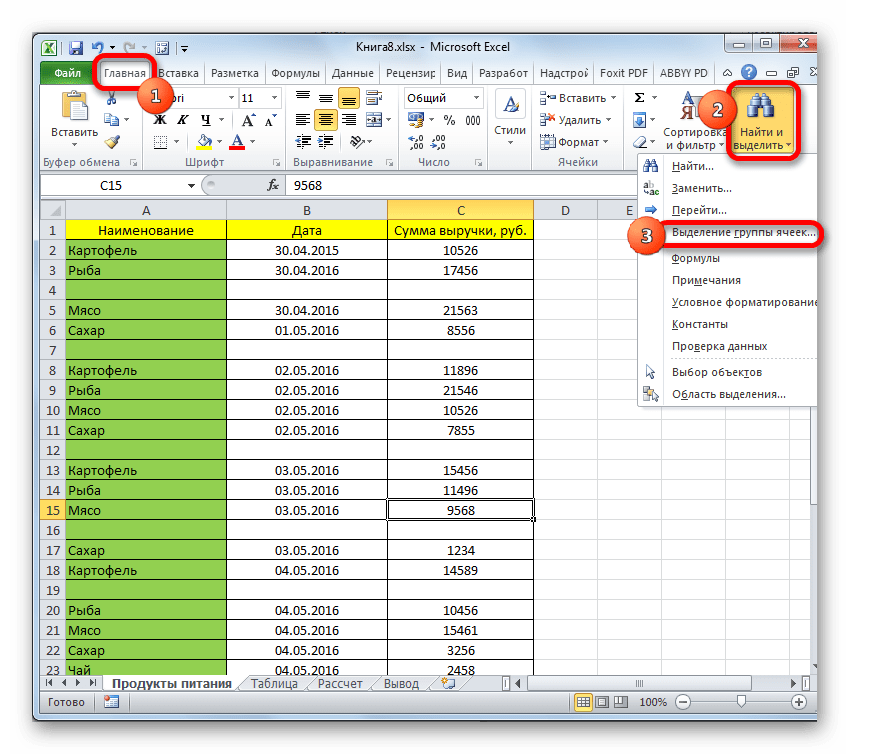
- Переходим во вкладку «Главная». На ленте инструментов жмем на значок «Найти и выделить». Он расположен в группе «Редактирование». В открывшемся списке жмем на пункт «Выделение группы ячеек».
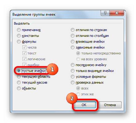
- Запускается небольшое окошко выделения группы ячеек. Ставим в нем переключатель в позицию «Пустые ячейки». После этого жмем на кнопку «OK».
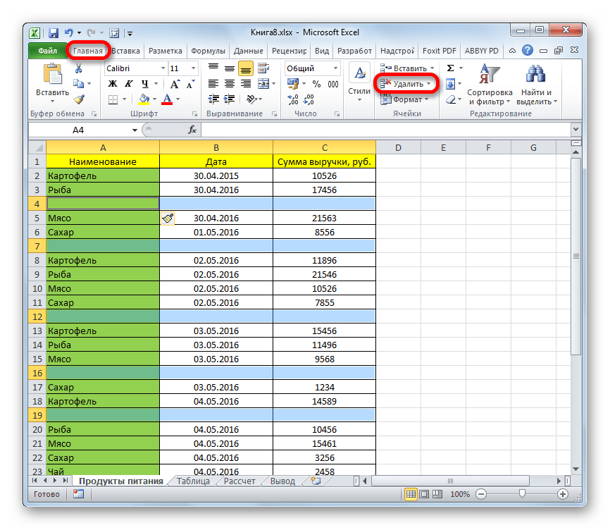
- Как видим, после того, как мы применили данное действие, все пустые элементы выделены. Теперь можно использовать для их удаления любой из способов, о которых шла речь выше. Например, можно нажать на кнопку «Удалить», которая расположена на ленте в той же вкладке «Главная», где мы сейчас работаем.
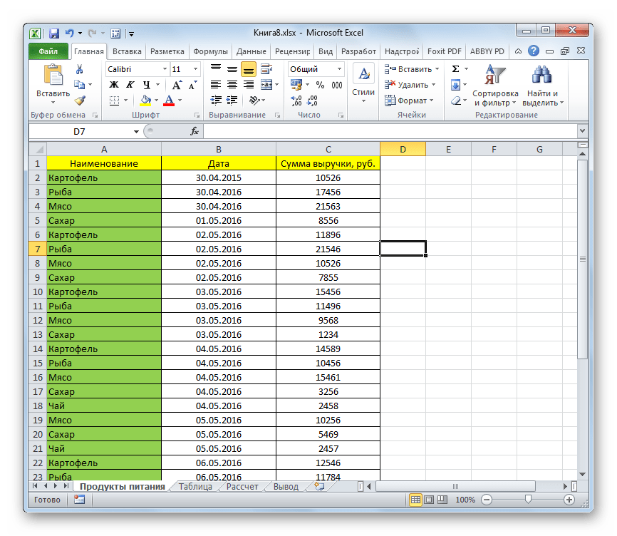
Как видим, все незаполненные элементы таблицы были удалены.
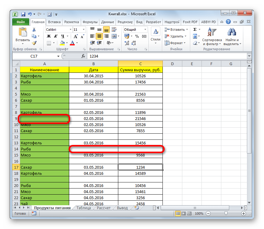
Обратите внимание! При использовании данного метода строчка должна быть абсолютно пустая. Если в таблице имеются пустые элементы, расположенные в строке, которая содержит какие-то данные, как на изображении ниже, этот способ применять нельзя. Его использование может повлечь сдвиг элементов и нарушение структуры таблицы.
Урок: Как удалить пустые строки в Экселе
Способ 5: использование сортировки
Для того, чтобы убрать строки по определенному условию можно применять сортировку. Отсортировав элементы по установленному критерию, мы сможем собрать все строчки, удовлетворяющие условию вместе, если они разбросаны по всей таблице, и быстро убрать их.
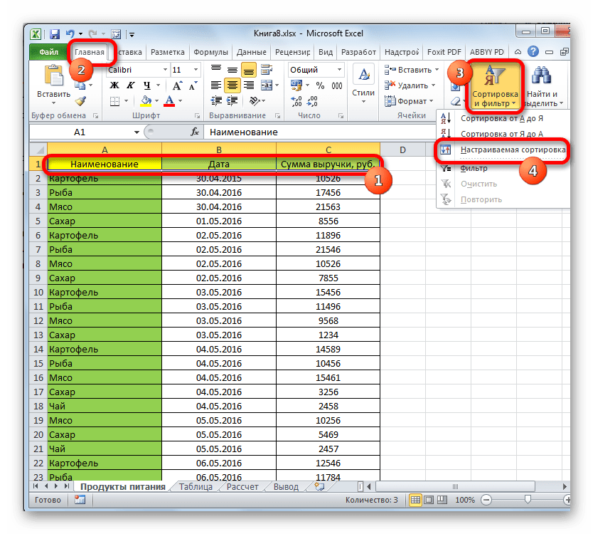
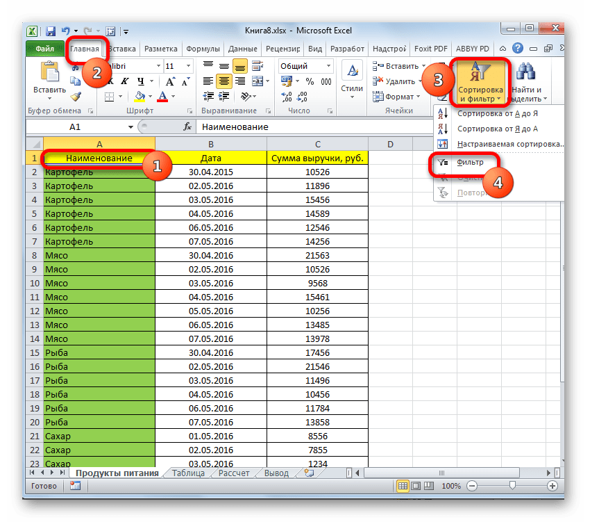
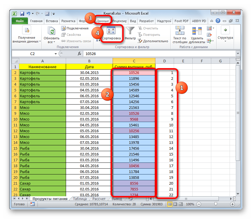
- Выделяем всю область таблицы, в которой следует провести сортировку, или одну из её ячеек. Переходим во вкладку «Главная» и кликаем по значку «Сортировка и фильтр», которая расположена в группе «Редактирование». В открывшемся списке вариантов действий выбираем пункт «Настраиваемая сортировка».

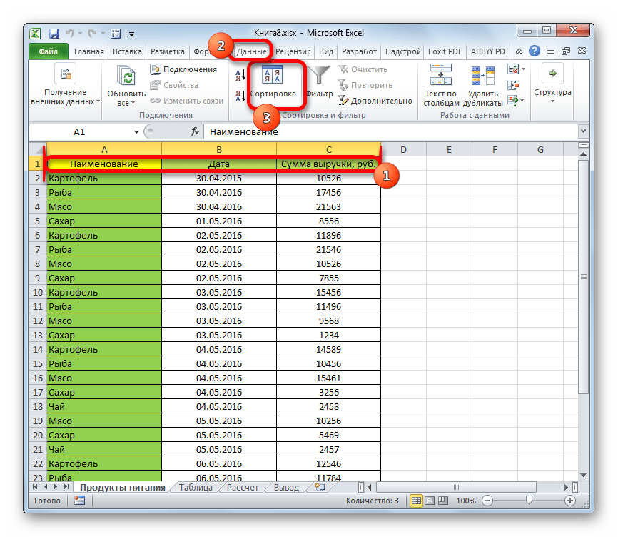
Можно также совершить альтернативные действия, которые тоже приведут к открытию окна настраиваемой сортировки. После выделения любого элемента таблицы переходим во вкладку «Данные». Там в группе настроек «Сортировка и фильтр» жмем на кнопку «Сортировка».
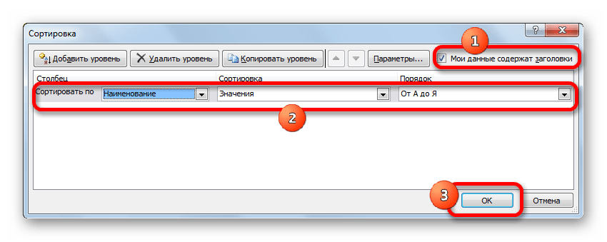
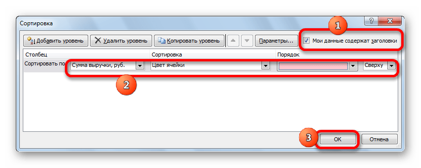
- Запускается окно настраиваемой сортировки. Обязательно установите галочку, в случае её отсутствия, около пункта «Мои данные содержат заголовки», если у вашей таблицы имеется шапка. В поле «Сортировать по» нужно выбрать наименование столбца, по которому будет происходить отбор значений для удаления. В поле «Сортировка» нужно указать, по какому именно параметру будет происходить отбор:
- Значения;
- Цвет ячейки;
- Цвет шрифта;
- Значок ячейки.
Тут уже все зависит от конкретных обстоятельств, но в большинстве случаев подходит критерий «Значения». Хотя в дальнейшем мы поговорим и об использовании другой позиции.
В поле «Порядок» нужно указать, в каком порядке будут сортироваться данные. Выбор критериев в этом поле зависит от формата данных выделенного столбца. Например, для текстовых данных порядок будет «От А до Я» или «От Я до А», а для даты «От старых к новым» или «От новых к старым». Собственно сам порядок большого значения не имеет, так как в любом случае интересующие нас значения будут располагаться вместе.
После того, как настройка в данном окне выполнена, жмем на кнопку «OK». - Все данные выбранной колонки будут отсортированы по заданному критерию. Теперь мы можем выделить рядом находящиеся элементы любым из тех вариантов, о которых шла речь при рассмотрении предыдущих способов, и произвести их удаление.
Кстати, этот же способ можно использовать для группировки и массового удаления пустых строчек.
Внимание! Нужно учесть, что при выполнении такого вида сортировки, после удаления пустых ячеек положение строк будет отличаться от первоначального. В некоторых случаях это не важно. Но, если вам обязательно нужно вернуть первоначальное расположение, то тогда перед проведением сортировки следует построить дополнительный столбец и пронумеровать в нем все строчки, начиная с первой. После того, как нежелательные элементы будут удалены, можно провести повторную сортировку по столбцу, где располагается эта нумерация от меньшего к большему. В таком случае таблица приобретет изначальный порядок, естественно за вычетом удаленных элементов.
Урок: Сортировка данных в Экселе
Способ 6: использование фильтрации
Для удаления строк, которые содержат определенные значения, можно также использовать такой инструмент, как фильтрация. Преимущество данного способа состоит в том, что, если вам вдруг эти строчки когда-нибудь понадобится снова, то вы их сможете всегда вернуть.
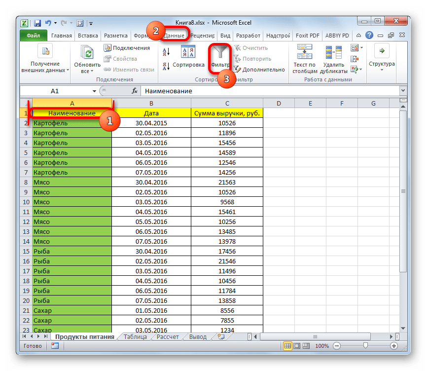
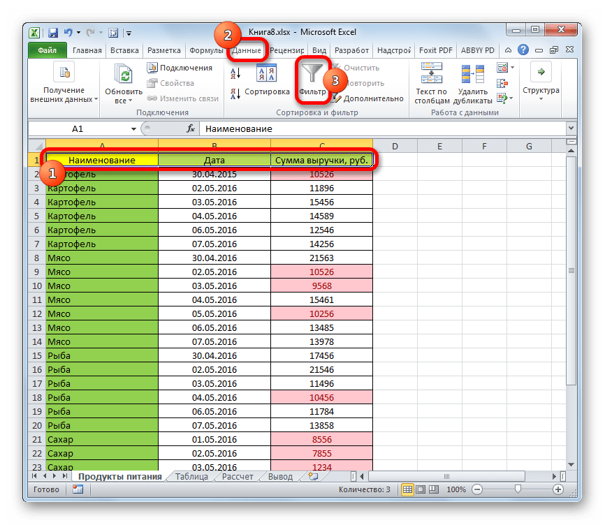
- Выделяем всю таблицу или шапку курсором с зажатой левой кнопкой мыши. Кликаем по уже знакомой нам кнопке «Сортировка и фильтр», которая расположена во вкладке «Главная». Но на этот раз из открывшегося списка выбираем позицию «Фильтр».

Как и в предыдущем способе, задачу можно также решить через вкладку «Данные». Для этого, находясь в ней, нужно щелкнуть по кнопке «Фильтр», которая расположена в блоке инструментов «Сортировка и фильтр».
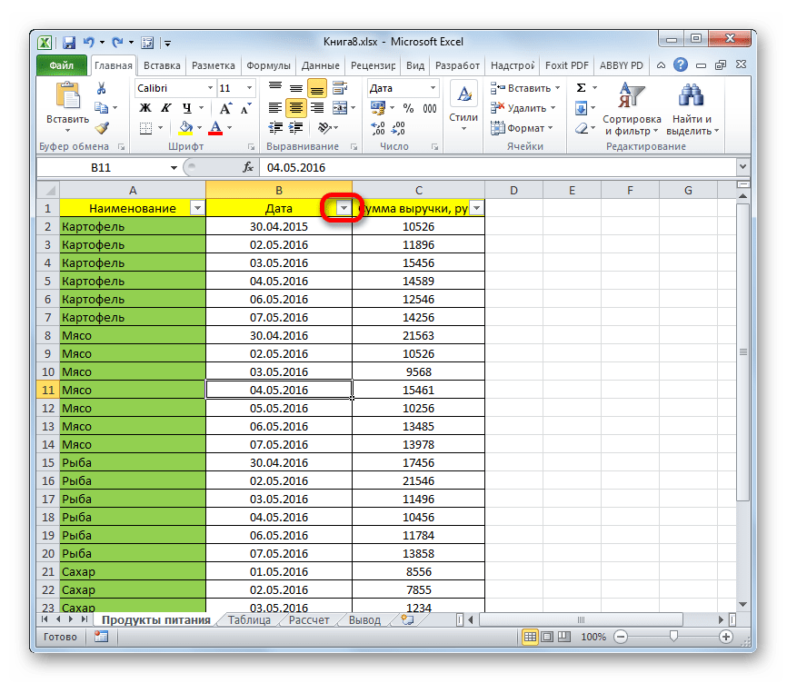
- После выполнения любого из вышеуказанных действий около правой границы каждой ячейки шапки появится символ фильтрации в виде треугольника, направленного углом вниз. Жмем по этому символу в том столбце, где находится значение, по которому мы будем убирать строки.
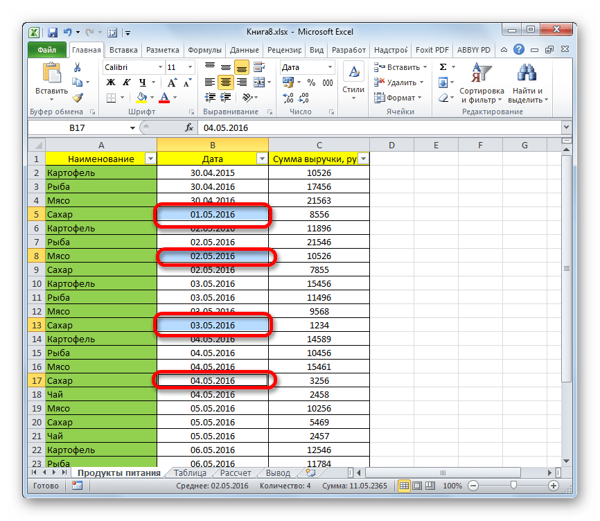
- Открывается меню фильтрования. Снимаем галочки с тех значений в строчках, которые хотим убрать. После этого следует нажать на кнопку «OK».
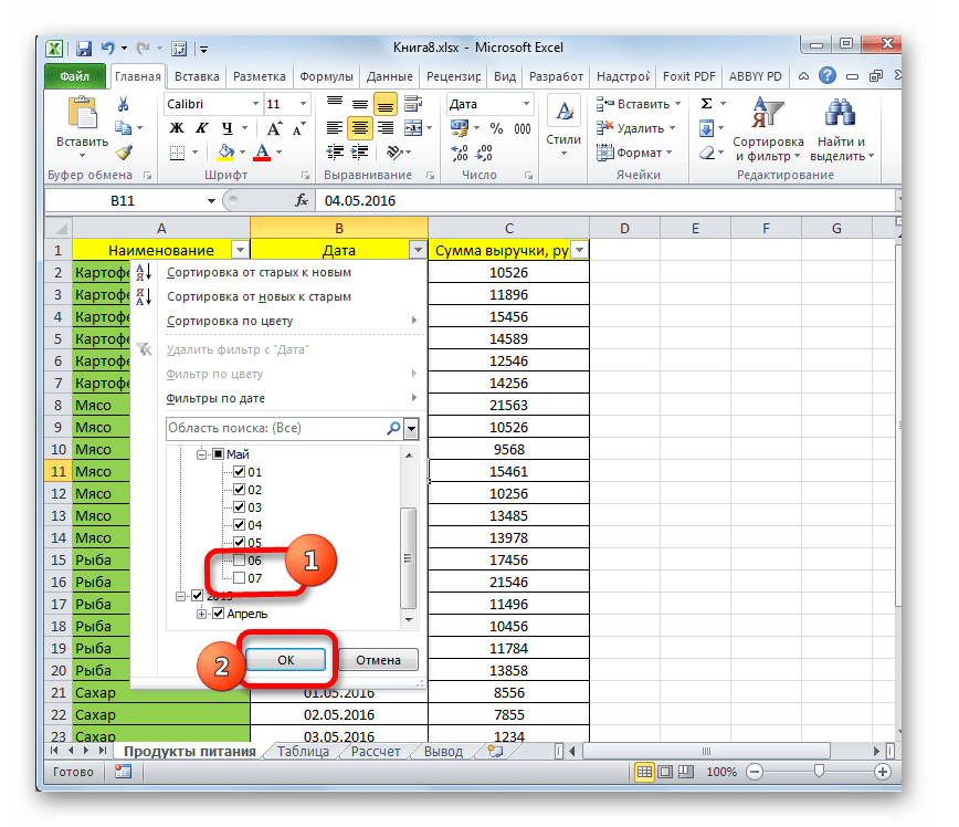
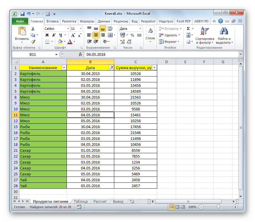
Таким образом, строки, содержащие значения, с которых вы сняли галочки, будут спрятаны. Но их всегда можно будет снова восстановить, сняв фильтрацию.
Урок: Применение фильтра в Excel
Способ 7: условное форматирование
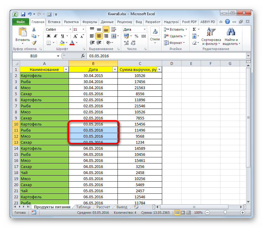
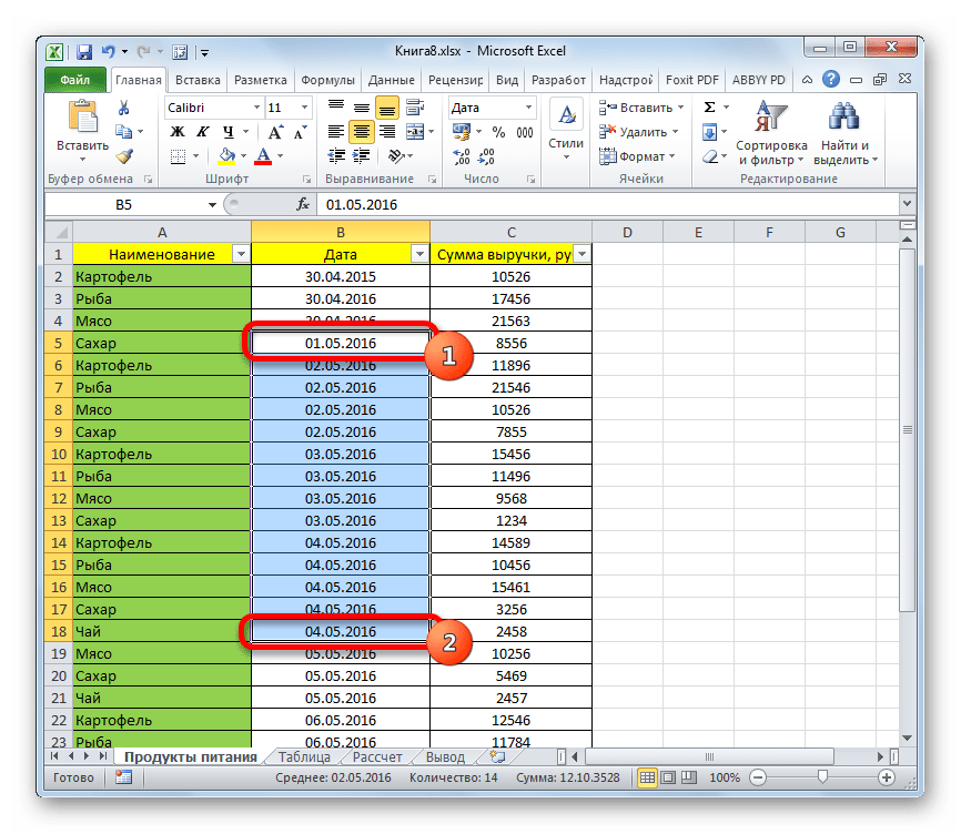
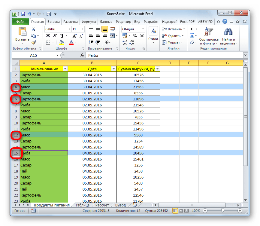
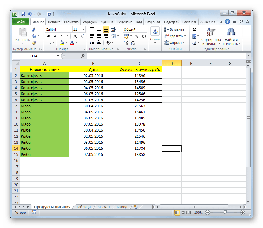
Ещё более точно можно задать параметры выбора строк, если вместе с сортировкой или фильтрацией использовать инструменты условного форматирования. Вариантов ввода условий в этом случае очень много, поэтому мы рассмотрим конкретный пример, чтобы вы поняли сам механизм использования этой возможности. Нам нужно удалить строчки в таблице, по которым сумма выручки менее 11000 рублей.
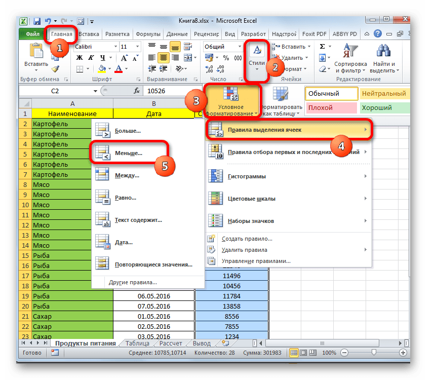
- Выделяем столбец «Сумма выручки», к которому хотим применить условное форматирование. Находясь во вкладке «Главная», производим щелчок по значку «Условное форматирование», который расположен на ленте в блоке «Стили». После этого открывается список действий. Выбираем там позицию «Правила выделения ячеек». Далее запускается ещё одно меню. В нем нужно конкретнее выбрать суть правила. Тут уже следует производить выбор, основываясь на фактической задаче. В нашем отдельном случае нужно выбрать позицию «Меньше…».
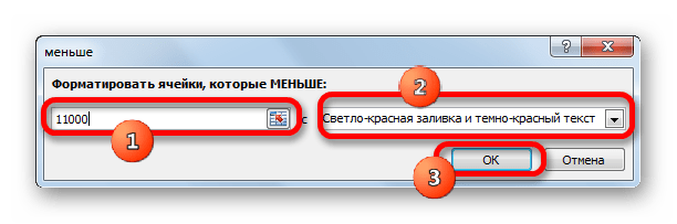
- Запускается окно условного форматирования. В левом поле устанавливаем значение 11000. Все значения, которые меньше него, будут отформатированы. В правом поле есть возможность выбрать любой цвет форматирования, хотя можно также оставить там значение по умолчанию. После того, как настройки выполнены, щелкаем по кнопке «OK».
- Как видим, все ячейки, в которых имеются значения выручки менее 11000 рублей, были окрашены в выбранный цвет. Если нам нужно сохранить изначальный порядок, после удаления строк делаем дополнительную нумерацию в соседнем с таблицей столбце. Запускаем уже знакомое нам окно сортировки по столбцу «Сумма выручки» любым из способов, о которых шла речь выше.
- Открывается окно сортировки. Как всегда, обращаем внимание, чтобы около пункта «Мои данные содержат заголовки» стояла галочка. В поле «Сортировать по» выбираем столбец «Сумма выручки». В поле «Сортировка» устанавливаем значение «Цвет ячейки». В следующем поле выбираем тот цвет, строчки с которым нужно удалить, согласно условному форматированию. В нашем случае это розовый цвет. В поле «Порядок» выбираем, где будут размещаться отмеченные фрагменты: сверху или снизу. Впрочем, это не имеет принципиального значения. Стоит также отметить, что наименование «Порядок» может быть смещено влево от самого поля. После того, как все вышеуказанные настройки выполнены, жмем на кнопку «OK».
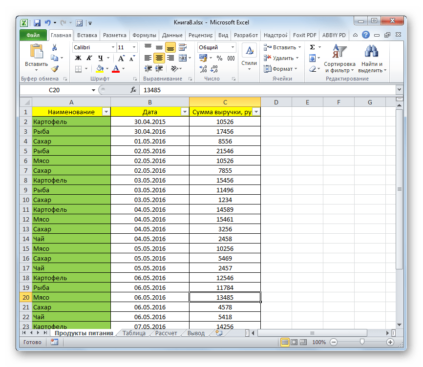
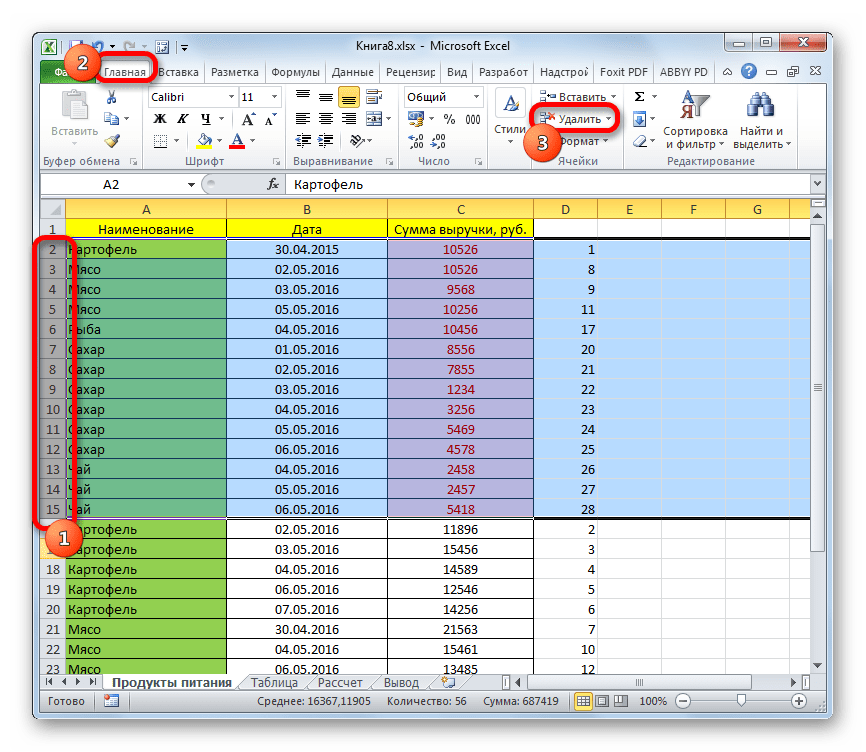
- Как видим, все строчки, в которых имеются выделенные по условию ячейки, сгруппированы вместе. Они будут располагаться вверху или внизу таблицы, в зависимости от того, какие параметры пользователь задал в окне сортировки. Теперь просто выделяем эти строчки тем методом, который предпочитаем, и проводим их удаление с помощью контекстного меню или кнопки на ленте.
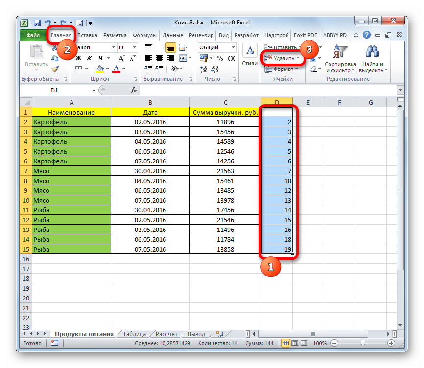
- Затем можно отсортировать значения по столбцу с нумерацией, чтобы наша таблица приняла прежний порядок. Ставший ненужным столбец с номерами можно убрать, выделив его и нажав знакомую нам кнопку «Удалить» на ленте.
Поставленная задача по заданному условию решена.
Кроме того, можно произвести аналогичную операцию с условным форматированием, но только после этого проведя фильтрацию данных.
- Итак, применяем условное форматирование к столбцу «Сумма выручки» по полностью аналогичному сценарию. Включаем фильтрацию в таблице одним из тех способов, которые были уже озвучены выше.
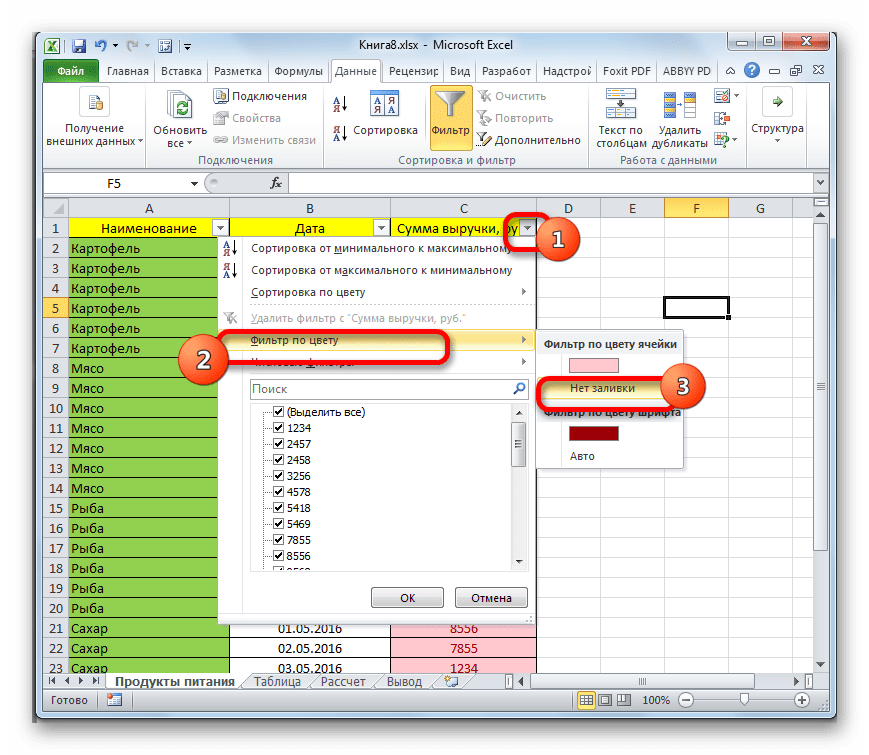
- После того, как в шапке появились значки, символизирующие фильтр, кликаем по тому из них, который расположен в столбце «Сумма выручки». В открывшемся меню выбираем пункт «Фильтр по цвету». В блоке параметров «Фильтр по цвету ячейки» выбираем значение «Нет заливки».
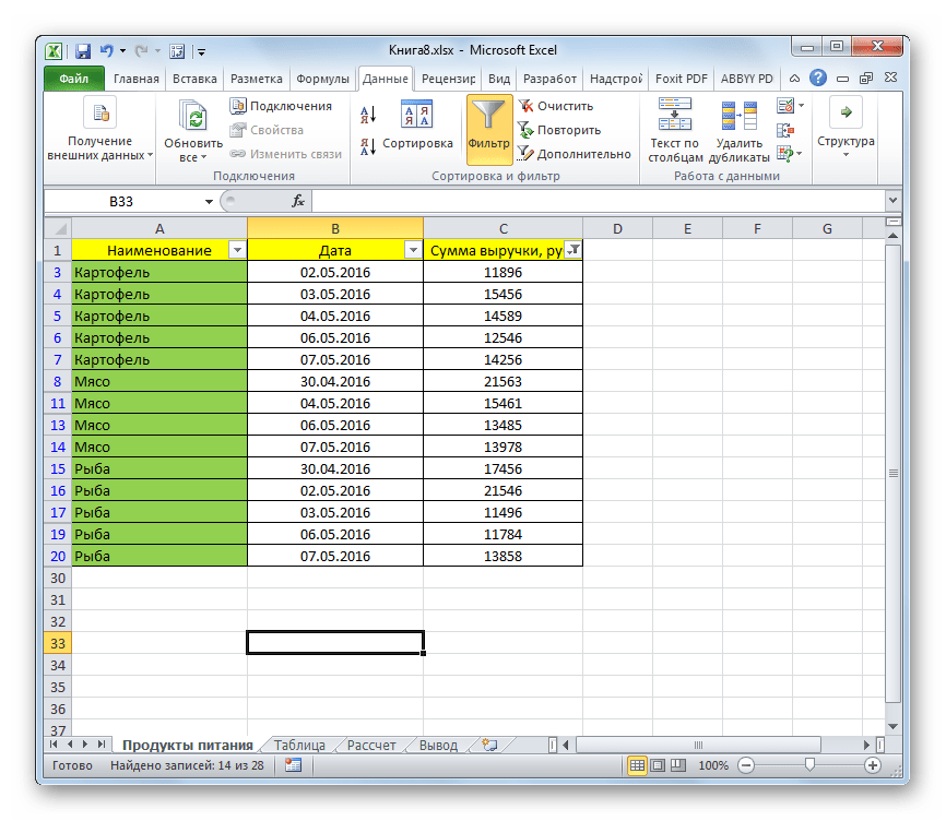
- Как видим, после этого действия все строчки, которые были залиты цветом с помощью условного форматирования, исчезли. Они спрятаны фильтром, но если удалить фильтрацию, то в таком случае, указанные элементы снова отобразятся в документе.
Урок: Условное форматирование в Экселе
Как видим, существует очень большое количество способов удалить ненужные строки. Каким именно вариантом воспользоваться зависит от поставленной задачи и от количества удаляемых элементов. Например, чтобы удалить одну-две строчки вполне можно обойтись стандартными инструментами одиночного удаления. Но чтобы выделить много строк, пустые ячейки или элементы по заданному условию, существуют алгоритмы действий, которые значительно облегчают задачу пользователям и экономят их время. К таким инструментам относится окно выделения группы ячеек, сортировка, фильтрация, условное форматирование и т.п.
Delete Row | Delete Rows | Delete Cells
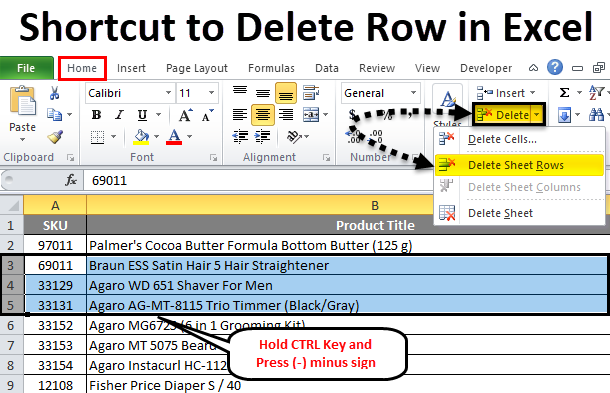
To quickly delete a row in Excel, select a row and use the shortcut CTRL — (minus sign). To quickly delete multiple rows, select multiple rows and use the same shortcut.
Delete Row
To delete a row in Excel, execute the following steps.
1. Select a row.

2. Right click, and then click Delete.

Result:

Note: instead of executing step 2, use the shortcut CTRL — (minus sign).
Delete Rows
To quickly delete multiple rows in Excel, execute the following steps.
1. Select multiple rows by clicking and dragging over the row headers.

2. Press CTRL — (minus sign).
Result:

Delete Cells
Excel displays the Delete Cells dialog box if you don’t select a row or multiple rows before using the shortcut CTRL — (minus sign).
1. Select cell A3.

2. Press CTRL — (minus sign).
3a. Excel automatically selects «Shift cells up». Click OK.

Result:

3b. To delete a row, select «Entire row» and click OK.

Result:

As you know, Excel is a very user-friendly software for daily business purpose data manipulation. In day-to-day data management, we maintain the data in Excel sheets. However, sometimes we need to delete the row and number of rows from the data. We can delete the selected row in Excel just by CTRL –(minus sign).
To delete multiple rows quickly, we can use the same shortcut.
Also, have a look at this list of Excel ShortcutsAn Excel shortcut is a technique of performing a manual task in a quicker way.read more.
Table of contents
- Shortcut to Delete Row in Excel
- How to Delete Row In Excel Shortcut?
- Deleting a Row Using Excel (ctrl -) Shortcut – Example #1
- Deleting a Row Using Right Click – Example #2
- Deleting the Multiple Rows – Example #3
- Things to Remember
- Recommended Articles
- How to Delete Row In Excel Shortcut?
How to Delete Row In Excel Shortcut?
Let us understand the Excel shortcut keys working with simple examples below.
You can download this Delete Row Excel Shortcut Template here – Delete Row Excel Shortcut Template
Deleting a Row Using Excel (ctrl -) Shortcut – Example #1
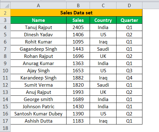
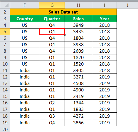
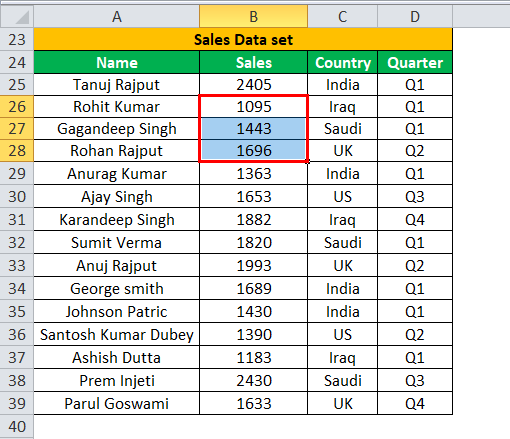
The table below shows a sales data set to apply the delete row in the Excel shortcut operation.
Below are the steps for deleting a row in Excel (CTRL -) shortcut:
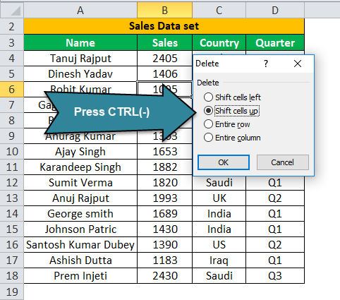
- We must first select the row we want to delete from the sales data table. Here, we pick row no.3.
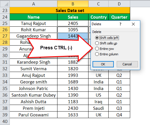
- Then, press the CTRL – (minus sign) keys.

- We may get the below four options to decide the place for the remaining data:
That are shift cells left
Shift cells up (by default)
Entire Row
Entire Column - We may select the whole row from the available option by pressing the “R” button, then the “OK” key.

- As a result, row no.3 will be deleted from the given data set.

Deleting a Row Using Right Click – Example #2
Let us consider the below country-wise sales data, and we want to delete row 2 from it.
Now, we must select row no. 2 and right-click and choose the “Delete” option, as shown below.
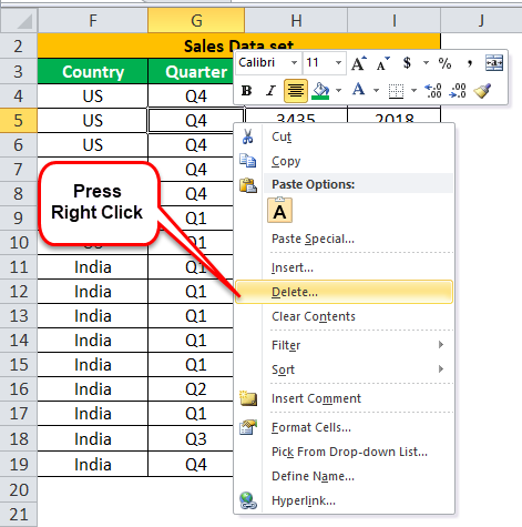
As a result, it will enable the below four options to decide the place for the remaining data:
- Shift cells left.
- Shift cells up (by default)
- Entire Row
- Entire Column
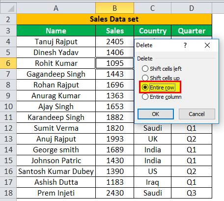
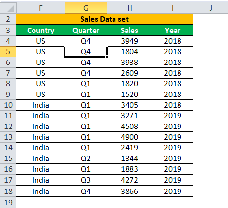
Select the “Entire Row” from the available option and press the “OK” key.
The output will be:
Deleting the Multiple Rows – Example #3
This example will apply the shortcut key on multiple rows at once.
Let us consider the table below and select the multiple rows from the table we want to delete from this table. For example, suppose we want to delete the 3rd,4th, and 5th rows from the below table.
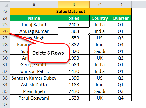
Then, select the 3rd,4th, and 5th rows and press the CTRL-
Now, we must choose the “Entire Row” and click “OK.”
And we will get the below table after deletion.
Things to Remember
- We must always select the “Entire Row” option while deleting the row. Otherwise, we may face the wrong data moving problem in your table.
- Suppose we select the “Shift cell up” option from the table, then only the cell from the table gets deleted, not the whole row, and our data from the cell below gets shifted upwards.
- Suppose we select the “Shift cell left” option from the table, then only the cell from the table gets deleted, not the whole row, and the entire row data gets shifted to the left.
- If we select the “Entire Column” option, the selected column will get deleted.
Recommended Articles
This article is a guide to keyboard Shortcut to Delete Row in Excel. Here, we discuss how to delete a row in Excel using shortcuts – 1) Using CTRL (-) 2) Using right-click, 3) Deleting the multiple rows along with practical examples. You may learn more about Excel from the following articles: –
- Insert Row in VBA
- Insert Row Shortcut in Excel
- Excel Delete Blank Rows
- Excel Create List
Excel Delete Row Shortcut (Table of Contents)
- Shortcut to Delete Row in Excel
- How to delete a row in excel using right-click menu without Shortcut
- How to delete the excel row using the ribbon menu
Shortcut to Delete Row in Excel
To delete a row in excel, we need to select the Rows which we want to delete and press Ctrl + Minus (“-“) sign together. This will eliminate the rows which we do not want. This can also be done by selecting the row in excel, choosing the Delete Row option available in the right-click menu list. We can even Delete a cell from any row by selecting Shift Cell Up from Right-click menu’s Delete option. This will move the data up by cells position, which we remove.
How to delete a row in excel using right-click menu without Shortcut
- First, select the row that you want to delete.
- Right-click on the row cell.
- We will get the dialog box.
- Click on delete so that the selected row will be deleted.
How to delete the excel row using the ribbon menu
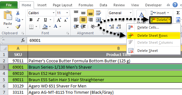
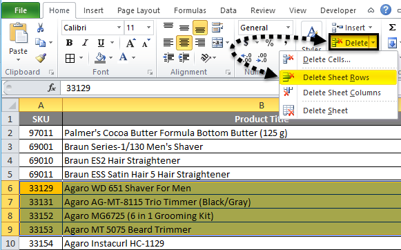
In Microsoft Excel, we can find the delete cells on the home menu, which is shown in the below screenshot.
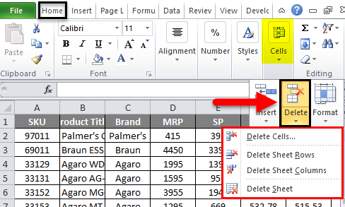
Once you click on the delete cells, we will get the following options:
- Delete cells: Which are used to delete the selected cells.
- Delete Sheet Rows: Which is used to delete the selected rows.
- Delete Sheet Column: Which is used to delete the selected column.
- Delete Sheet: Which is used to delete the entire sheet.
We will see all these options one by one.
Example #1 – Delete Cells
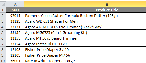
Consider the below example, which has sales data. Sometimes it is required to delete unwanted rows and columns in the data. So in this, we need to delete the cells which are shown in the below steps.
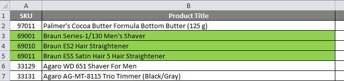
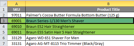
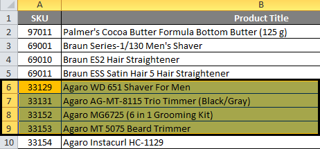
Assume that we need to delete the row that has been highlighted in green color.
- First, select the row you exactly need to delete, as shown in the below figure.
- Go to the delete cells. Click on the delete cells so that we will get the below delete option as shown in the below screenshot. Click on the second delete option called “delete sheet rows.”
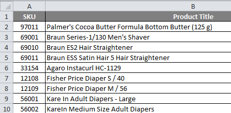
- So that the selected row will be deleted, as shown in the below screenshot
We can see the difference that the first column named SKU 69001 row has been deleted, and the count of a row highlighted in green color has been reduced to two rows before the highlighted green color row count was three.
Example #2 – How to delete entire selected rows
In this example, we are going to see how to delete the entire row by following the below steps.
Here we need to delete the highlighted rows.
- First, select the highlighted row that we need to delete, as shown in the below screenshot.
- Now click on the delete cells. Click on the second delete options, “ delete sheet rows.”
- So that the selected entire row sheets will be deleted, which is shown in the below output.
In the above screenshot, we can see that selected rows have been deleted to see the difference that highlighted rows had been deleted.
Example #3
(a) Use Keyboard shortcut to delete the row in excel
In Microsoft Excel, we have several shortcut keys for all functions where we have a shortcut key for deleting the excel row and column also. The shortcut key for deleting the row in excel is CTRL +” -”( minus sign), and the shortcut key for inserting the row is CTRL +SHIFT+ ” +” (plus sign), and the same shortcuts can be used for inserting and deleting for the same. Mostly we will be using the number pad for inserting numbers. We can also use the number pad shortcut key to delete the row. The shortcut key to be applied is CTRL+”+”(Plus Sign).
Steps to use shortcut keys to delete the row in excel
The keyboard shortcut key to delete the row in excel is CTRL+ “-“i.e. Minus sign which we need to use.
- First, select the cell where you exactly need to delete the row, which is shown below.
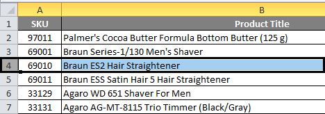
- Use the keyboard shortcut key. Hold CTRL Key and Press “-“ minus sign on the keyboard.
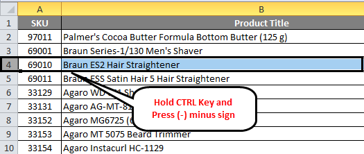
- So that the entire row will be deleted, which is shown below.
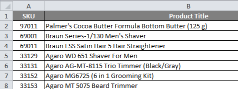
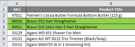
Here we can see the difference that the Product title name “Braun ES2 Hair Straightener “ row has been deleted, as we notice that in the above screenshot.
(b) How to Delete Entire Rows in Excel Using the Keyboard Shortcut key
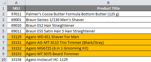
Consider the below example where we need to delete rows of the brand name “ BRAUN”, which is highlighted for reference.
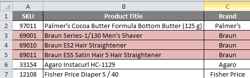
In order to delete the excel rows using a keyboard shortcut, follow the below steps.
- First, select the row cells which has been highlighted in pink color.
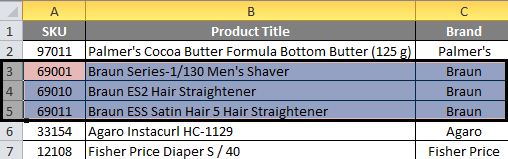
- Press the CTRL key and hold it. By holding the CTRL key, press the “-“ minus sign.
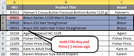
- Once you press the CTRL key and – key at a time, the selected row will be deleted. We will get the below result which is shown in the below screenshot.
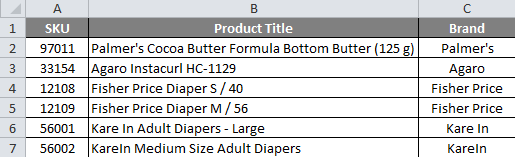
We can see that the BRAND name called “BRAUN” rows has been completely deleted in the above screenshot.
Example #4 – Deleting Selected and Multiple Rows in Excel
Consider the below example where we can see unwanted blank rows in the sheet that makes the data inappropriate. In this scenario, we can delete the blank rows at a time using the keyboard shortcut or using the delete cells menu.
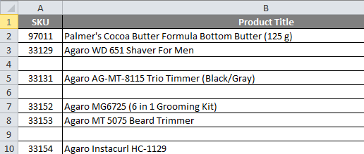
Now we need to delete the blank rows in the above sales data and make the sheet with clear input.
In order to delete the multiple rows at a time, follow the below simple steps.
- First, hold the CTRL Key.
- Select the entire blank rows by holding the CTRL-key.
- We can see that selected rows have been marked in blue color.
- Now go to delete cells. Click on delete sheet rows.
- Once you click on the delete sheet rows, all the selected rows will be deleted within a fraction of a second.
- We will get the result as follows, which is given below.
In the above screenshot, we can notice that all blank rows are now deleted, and the data looks better when compared to previous data.
Things to Remember About Delete Row Excel Shortcut
While deleting the data in excel, make sure that the data is not required. However, we can retrieve the deleted rows by doing undo in excel.
You can download this Delete Row Shortcut Excel Template here – Delete Row Shortcut Excel Template.
Recommended Articles
This has been a guide to shortcut to delete a row in excel. Here we discuss how to delete a row in excel using a shortcut – 1) keyboard shortcut 2) Using Right Click 3) Using Delete Sheet Row option along with practical examples and downloadable excel template. You can also go through our other suggested articles –
- ROWS Function in Excel
- VBA Delete Row
- Remove (Delete) Blank Rows in Excel
- Excel Rows and Columns
While working in Excel we have to take so many actions and activities in which insertion and deletion is most commonly used. In this article, we will learn how we can insert and delete a Row/Column in Microsoft Excel by using the shortcut key.
Let’s take an example to understand how to insert or delete a Row/Column.
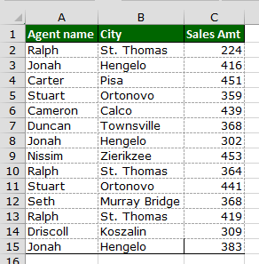
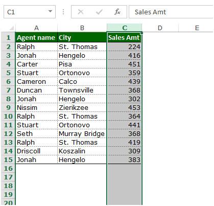
We have data in range A1: C15. Column A contains Agent name, column B contains city, column C contains sales amount, and we need to return the total value in cell C16.
Insert row in data
Follow below given steps:-
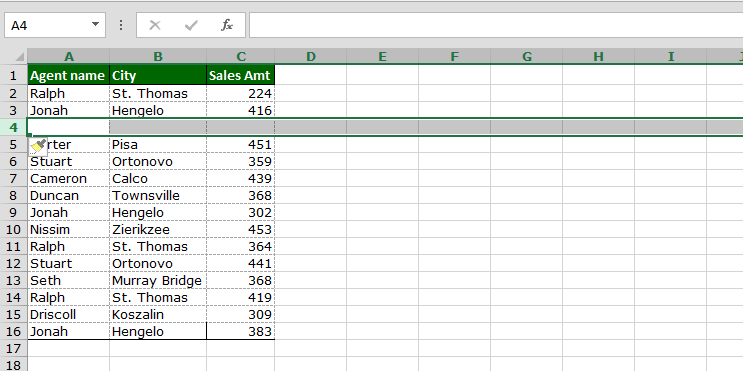
- We want to insert the row in between 3rd and 4th row.
- Select the 4th row and press the key Ctrl+ on your keyboard.

- Row will get inserted in between 3rd and 4th row.
Delete entire row in data
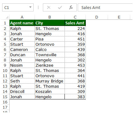
- To delete the 4th row, select the 4th row.
- The Excel delete row shortcut is press Ctrl+- (Ctrl with minus) key on your keyboard.
- Row will get deleted from the data.
Insert and Delete Column in data
Follow below given steps:-
- We want to insert a Column in between B and C column.
- Select the column C and press the key Ctrl+ on your keyboard.
- Column will get inserted in between B and C column.

- To delete the C column, select the Column C.

- And press Ctrl+- (Ctrl with minus) key on your keyboard.
- Column will get deleted from the data.
This is the way we can insert and delete a row/column in Microsoft Excel.
![]()
If you liked our blogs, share it with your friends on Facebook. And also you can follow us on Twitter and Facebook.
We would love to hear from you, do let us know how we can improve, complement or innovate our work and make it better for you. Write us at info@exceltip.com
Bottom line: Learn some of my favorite keyboard shortcuts when working with rows and columns in Excel.
Skill level: Easy
Whether you are creating a simple list of names or building a complex financial model, you probably make a lot of changes to the rows and columns in the spreadsheet. Tasks like adding/deleting rows, adjusting column widths, and creating outline groups are very common when working with the grid.
This post contains some of my favorite shortcuts that will save you time every day.
I’ve also listed the equivalent shortcuts for the Mac version of Excel where available.
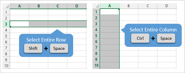
#1 – Select Entire Row or Column
Shift+Space is the keyboard shortcut to select an entire row.
Ctrl+Space is the keyboard shortcut to select an entire column.
Mac Shortcuts: Same as above
The keyboard shortcuts by themselves don’t do much. However, they are the starting point for performing a lot of other actions where you first need to select the entire row or column. This includes tasks like deleting rows, grouping columns, etc.
These shortcuts also work for selecting the entire row or column inside an Excel Table.
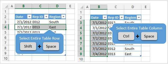
When you press the Shift+Space shortcut the first time it will select the entire row within the Table. Press Shift+Space a second time and it will select the entire row in the worksheet.
The same works for columns. Ctrl+Space will select the column of data in the Table. Pressing the keyboard shortcut a second time will include the column header of the Table in the selection. Pressing Ctrl+Space a third time will select the entire column in the worksheet.
You can select multiple rows or columns by holding Shift and pressing the Arrow Keys multiple times.
![]()
#2 – Insert or Delete Rows or Columns
There are a few ways to quickly delete rows and columns in Excel.
If you have the rows or columns selected, then the following keyboard shortcuts will quickly add or delete all selected rows or columns.
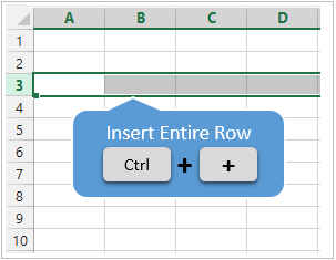
Ctrl++ (plus character) is the keyboard shortcut to insert rows or columns. If you are using a laptop keyboard you can press Ctrl+Shift+= (equal sign).
Mac Shortcut: Cmd++ or Cmd+Shift+
Ctrl+- (minus character) is the keyboard shortcut to delete rows or columns.
Mac Shortcut: Cmd+-
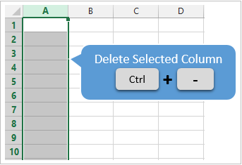
So for the above shortcuts to work you will first need to select the entire row or column, which can be done with the Shift+Space or Ctrl+Space shortcuts explained in #1.
If you do not have the entire row or column selected then you will be presented with the Insert or Delete Menus after pressing Ctrl++ or Ctrl+-.
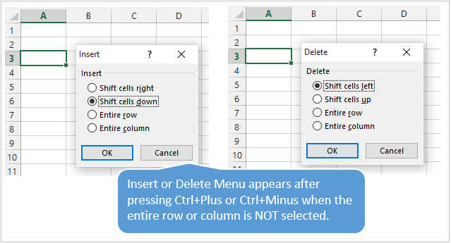
You can then press the up or down arrow keys to make your selection from the menu and hit Enter. For me it is easier to first select the entire row or column, then press Ctrl++ or Ctrl+-.
So, the entire keyboard shortcut to delete a column would be Ctrl+Space, Ctrl+-. You could also use the keyboard shortcut Alt+H+D+C to delete columns and Alt+H+D+R to delete rows. There are lots of ways to do a simple task… 🙂
#3 – AutoFit Column Width
There are also a lot of different ways to AutoFit column widths. AutoFit means that the width of the column will be adjusted to fit the contents of the cell.
You can use the mouse and double-click when you hover the cursor between columns when you see the resize column cursor.
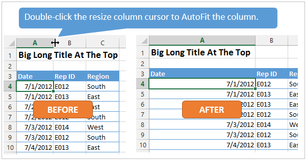
The problem with this is that you might just want to resize the column for the date in cell A4, instead of the big long title in cell A1. To accomplish this you can use the AutoFit Column Width button. It is located on the Home tab of the Ribbon in the Format menu.
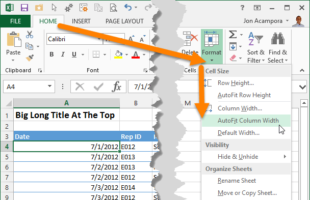
The AutoFit Column Width button bases the width of the column on the cells you have selected. In the image above I have cell A4 selected. So the column width will be adjusted to fit the contents of A4, as shown in the results below.
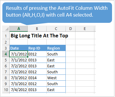
Alt,H,O,I is the keyboard shortcut for the AutoFit Column Width button. This is one I use a lot to get my reports looking shiny. 🙂
Alt,H,O,A is the keyboard shortcut to AutoFit Row Height. It doesn’t work exactly the same as column width, and will only adjust the row height to the tallest cell in the entire row.
Mac Shortcuts: None that I know of. The Mac version does not use the Alt key sequence which I believe is a limitation of the Mac OS.
#3.5 – Manually Adjust Row or Column Width
The column width or row height windows can be opened with keyboard shortcuts as well.
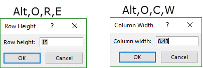
Alt,O,R,E is the keyboard shortcut to open the Row Height window.
Alt,O,C,W is the keyboard shortcut to open the Column Width window.
The row height or column width will be applied to the rows or columns of all the cells that are currently selected.
These are old shortcuts from Excel 2003, but they still work in the modern versions of Excel.
Mac Shortcuts: None that I know of. The Mac version does not use the Alt key sequence which I believe is a limitation of the Mac OS.
#4 – Hide or Unhide Rows or Columns
There are several dedicated keyboard shortcuts to hide and unhide rows and columns.
- Ctrl+9 to Hide Rows
- Ctrl+0 (zero) to Hide Columns
- Ctrl+Shift+( to Unhide Rows
- Ctrl+Shift+) to Unhide Columns – If this doesn’t work for you try Alt,O,C,U (old Excel 2003 shortcut that still works). You can also modify a Windows setting to prevent the conflict with this shortcut. See the comment from Pablo Baez on Oct 5, 2015 below for further instructions. Thanks Pablo! 🙂
Mac Shortcuts: Same as above
The buttons are also located on the Format menu on the Home tab of the Ribbon. You can hover over any of the items in the menu and the keyboard shortcut will display in the screentip (see screenshot below).
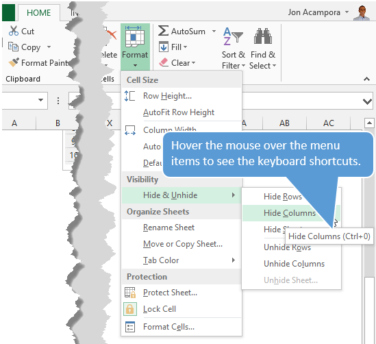
The trick with getting these shortcuts to work is to have the proper cells selected first.
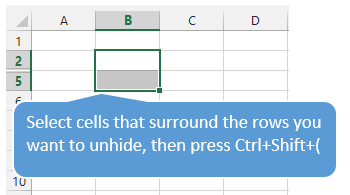
To hide rows or columns you just need to select cells in the rows or columns you want to hide, then press the Ctrl+9 or Ctrl+Shift+( shortcut.
To unhide rows or columns you first need to select the cells that surround the rows or columns you want to unhide. In the screenshot below I want to unhide rows 3 & 4. I first select cell B2:B5, cells that surround or cover the hidden rows, then press Ctrl+Shift+( to unhide the rows.
The same technique works to unhide columns.
#5 – Group or Ungroup Rows or Columns
Row and Column groupings are a great way to quickly hide and unhide columns and rows.
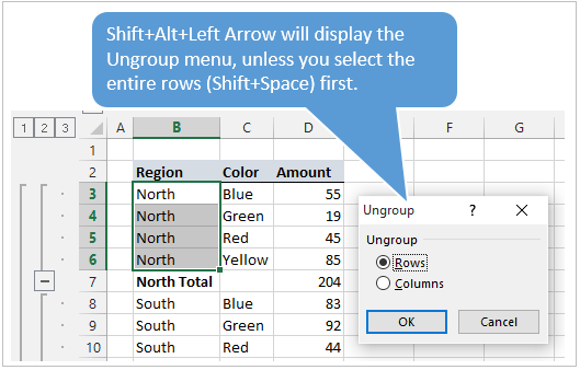
Shift+Alt+Right Arrow is the shortcut to group rows or columns.
Mac Shortcut: Cmd+Shift+K
Shift+Alt+Left Arrow is the shortcut to ungroup.
Mac Shortcut: Cmd+Shift+J
Again, the trick here is to select the entire rows or columns you want to group/ungroup first. Otherwise you will be presented with the Group or Ungroup menu.
Alt,A,U,C is the keyboard shortcut to remove all the row and columns groups on the sheet. This is the same as pressing the Clear Outline button on the Ungroup menu of the Data tab on the Ribbon.
*Bonus funny: At some point when using the group/ungroup shortcuts, you will accidentally press Ctrl+Alt+Right Arrow. This is a Windows shortcut that orientates the entire screen to the right. I call it “neck ache view”. To get it back to normal press Ctrl+Alt+Up Arrow.
If your co-worker or boss accidentally leaves their computer unlocked and you want to play a joke on them, press Ctrl+Alt+Down Arrow. This will turn their screen upside down. Don’t forget to record a video of their WTF reaction… 🙂
What Are Your Favorites?
There are a ton of keyboard shortcuts for working with rows and columns. The above are some of my favorites that I use everyday. What are some of your favorites? Please leave a comment below. Thanks! 🙂
Transcript
In this lesson, we’ll look at how to insert and delete rows in Excel. It’s common to insert rows to make room for more information. Deleting rows is an easy way to remove information you no longer want or need.
No matter how many rows you add or delete, the number of rows in the worksheet never changes. When you insert rows, rows are pushed off the worksheet at the bottom. When you delete rows, new rows are added to the bottom.
Let’s take a look.
To insert a row in Excel, first select the row below where you want the new row to be.
Then, click the Insert button on the ribbon.
Excel will always insert rows above your selection.
You can also right-click and choose Insert from the menu, which is generally faster.
If you’d like to insert multiple rows, just select more than one row before you insert. Excel will insert as many rows as you have selected.
To delete a row in Excel, first select the row you’d like to delete.
You can then delete the row using the ribbon or by right-clicking. To use the ribbon, click the Delete button.
To use your mouse, right-click and choose Delete from the menu.
You can delete multiple rows in the same way.

This Excel tutorial explains how to delete a row in Excel 2016 (with screenshots and step-by-step instructions).
Question:In Microsoft Excel 2016, how do I delete a row in a spreadsheet?
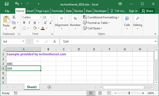
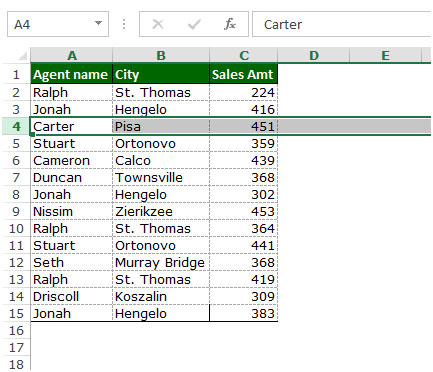
Answer: Select a cell in the row that you wish to delete. In this example, we have selected cell A4 because we want to delete row 4.

Right-click and select «Delete» from the popup menu.
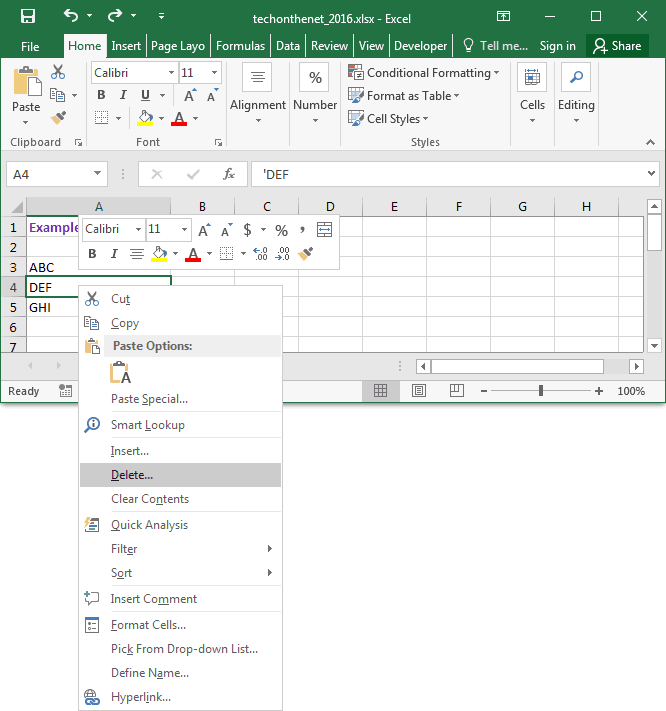
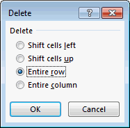
When the Delete window appears, select the «Entire row» option and click on the OK button.
The row should now be deleted in the spreadsheet. As you can see, one row has been removed (ie: row that was previously in row 4) and the rows below it have been shifted up.