
For quick access to related information in another file or on a web page, you can insert a hyperlink in a worksheet cell. You can also insert links in specific chart elements.
Note: Most of the screen shots in this article were taken in Excel 2016. If you have a different version your view might be slightly different, but unless otherwise noted, the functionality is the same.
-
On a worksheet, click the cell where you want to create a link.
You can also select an object, such as a picture or an element in a chart, that you want to use to represent the link.
-
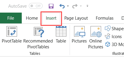
On the Insert tab, in the Links group, click Link
 .
.
You can also right-click the cell or graphic and then click Link on the shortcut menu, or you can press Ctrl+K.
-
-
Under Link to, click Create New Document.
-
In the Name of new document box, type a name for the new file.
Tip: To specify a location other than the one shown under Full path, you can type the new location preceding the name in the Name of new document box, or you can click Change to select the location that you want and then click OK.
-
Under When to edit, click Edit the new document later or Edit the new document now to specify when you want to open the new file for editing.
-
In the Text to display box, type the text that you want to use to represent the link.
-
To display helpful information when you rest the pointer on the link, click ScreenTip, type the text that you want in the ScreenTip text box, and then click OK.
 .
.-
On a worksheet, click the cell where you want to create a link.
You can also select an object, such as a picture or an element in a chart, that you want to use to represent the link.
-
On the Insert tab, in the Links group, click Link
.
You can also right-click the cell or object and then click Link on the shortcut menu, or you can press Ctrl+K.
-
-
Under Link to, click Existing File or Web Page.
-
Do one of the following:
-
To select a file, click Current Folder, and then click the file that you want to link to.
You can change the current folder by selecting a different folder in the Look in list.
-
To select a web page, click Browsed Pages and then click the web page that you want to link to.
-
To select a file that you recently used, click Recent Files, and then click the file that you want to link to.
-
To enter the name and location of a known file or web page that you want to link to, type that information in the Address box.
-
To locate a web page, click Browse the Web
, open the web page that you want to link to, and then switch back to Excel without closing your browser.
-
-
If you want to create a link to a specific location in the file or on the web page, click Bookmark, and then double-click the bookmark that you want.
Note: The file or web page that you are linking to must have a bookmark.
-
In the Text to display box, type the text that you want to use to represent the link.
-
To display helpful information when you rest the pointer on the link, click ScreenTip, type the text that you want in the ScreenTip text box, and then click OK.
 , open the web page that you want to link to, and then switch back to Excel without closing your browser.
To link to a location in the current workbook or another workbook, you can either define a name for the destination cells or use a cell reference.
-
To use a name, you must name the destination cells in the destination workbook.
How to name a cell or a range of cells
-
Select the cell, range of cells, or nonadjacent selections that you want to name.
-
Click the Name box at the left end of the formula bar
.
Name box -
In the Name box, type the name for the cells, and then press Enter.
Note: Names can’t contain spaces and must begin with a letter.
-
-
On a worksheet of the source workbook, click the cell where you want to create a link.
You can also select an object, such as a picture or an element in a chart, that you want to use to represent the link.
-
On the Insert tab, in the Links group, click Link
.
You can also right-click the cell or object and then click Link on the shortcut menu, or you can press Ctrl+K.
-
-
Under Link to, do one of the following:
-
To link to a location in your current workbook, click Place in This Document.
-
To link to a location in another workbook, click Existing File or Web Page, locate and select the workbook that you want to link to, and then click Bookmark.
-
-
Do one of the following:
-
In the Or select a place in this document box, under Cell Reference, click the worksheet that you want to link to, type the cell reference in the Type in the cell reference box, and then click OK.
-
In the list under Defined Names, click the name that represents the cells that you want to link to, and then click OK.
-
-
In the Text to display box, type the text that you want to use to represent the link.
-
To display helpful information when you rest the pointer on the link, click ScreenTip, type the text that you want in the ScreenTip text box, and then click OK.
 .
.
 Name box
You can use the HYPERLINK function to create a link that opens a document that is stored on a network server, an intranet, or the Internet. When you click the cell that contains the HYPERLINK function, Excel opens the file that is stored at the location of the link.
Syntax
HYPERLINK(link_location,friendly_name)
Link_location is the path and file name to the document to be opened as text. Link_location can refer to a place in a document — such as a specific cell or named range in an Excel worksheet or workbook, or to a bookmark in a Microsoft Word document. The path can be to a file stored on a hard disk drive, or the path can be a universal naming convention (UNC) path on a server (in Microsoft Excel for Windows) or a Uniform Resource Locator (URL) path on the Internet or an intranet.
-
Link_location can be a text string enclosed in quotation marks or a cell that contains the link as a text string.
-
If the jump specified in link_location does not exist or can’t be navigated, an error appears when you click the cell.
Friendly_name is the jump text or numeric value that is displayed in the cell. Friendly_name is displayed in blue and is underlined. If friendly_name is omitted, the cell displays the link_location as the jump text.
-
Friendly_name can be a value, a text string, a name, or a cell that contains the jump text or value.
-
If friendly_name returns an error value (for example, #VALUE!), the cell displays the error instead of the jump text.
Examples
The following example opens a worksheet named Budget Report.xls that is stored on the Internet at the location named example.microsoft.com/report and displays the text «Click for report»:
=HYPERLINK(«http://example.microsoft.com/report/budget report.xls», «Click for report»)
The following example creates a link to cell F10 on the worksheet named Annual in the workbook Budget Report.xls, which is stored on the Internet at the location named example.microsoft.com/report. The cell on the worksheet that contains the link displays the contents of cell D1 as the jump text:
=HYPERLINK(«[http://example.microsoft.com/report/budget report.xls]Annual!F10», D1)
The following example creates a link to the range named DeptTotal on the worksheet named First Quarter in the workbook Budget Report.xls, which is stored on the Internet at the location named example.microsoft.com/report. The cell on the worksheet that contains the link displays the text «Click to see First Quarter Department Total»:
=HYPERLINK(«[http://example.microsoft.com/report/budget report.xls]First Quarter!DeptTotal», «Click to see First Quarter Department Total»)
To create a link to a specific location in a Microsoft Word document, you must use a bookmark to define the location you want to jump to in the document. The following example creates a link to the bookmark named QrtlyProfits in the document named Annual Report.doc located at example.microsoft.com:
=HYPERLINK(«[http://example.microsoft.com/Annual Report.doc]QrtlyProfits», «Quarterly Profit Report»)
In Excel for Windows, the following example displays the contents of cell D5 as the jump text in the cell and opens the file named 1stqtr.xls, which is stored on the server named FINANCE in the Statements share. This example uses a UNC path:
=HYPERLINK(«\FINANCEStatements1stqtr.xls», D5)
The following example opens the file 1stqtr.xls in Excel for Windows that is stored in a directory named Finance on drive D, and displays the numeric value stored in cell H10:
=HYPERLINK(«D:FINANCE1stqtr.xls», H10)
In Excel for Windows, the following example creates a link to the area named Totals in another (external) workbook, Mybook.xls:
=HYPERLINK(«[C:My DocumentsMybook.xls]Totals»)
In Microsoft Excel for the Macintosh, the following example displays «Click here» in the cell and opens the file named First Quarter that is stored in a folder named Budget Reports on the hard drive named Macintosh HD:
=HYPERLINK(«Macintosh HD:Budget Reports:First Quarter», «Click here»)
You can create links within a worksheet to jump from one cell to another cell. For example, if the active worksheet is the sheet named June in the workbook named Budget, the following formula creates a link to cell E56. The link text itself is the value in cell E56.
=HYPERLINK(«[Budget]June!E56», E56)
To jump to a different sheet in the same workbook, change the name of the sheet in the link. In the previous example, to create a link to cell E56 on the September sheet, change the word «June» to «September.»
When you click a link to an email address, your email program automatically starts and creates an email message with the correct address in the To box, provided that you have an email program installed.
-
On a worksheet, click the cell where you want to create a link.
You can also select an object, such as a picture or an element in a chart, that you want to use to represent the link.
-
On the Insert tab, in the Links group, click Link
.
You can also right-click the cell or object and then click Link on the shortcut menu, or you can press Ctrl+K.
-
-
Under Link to, click E-mail Address.
-
In the E-mail address box, type the email address that you want.
-
In the Subject box, type the subject of the email message.
Note: Some web browsers and email programs may not recognize the subject line.
-
In the Text to display box, type the text that you want to use to represent the link.
-
To display helpful information when you rest the pointer on the link, click ScreenTip, type the text that you want in the ScreenTip text box, and then click OK.
You can also create a link to an email address in a cell by typing the address directly in the cell. For example, a link is created automatically when you type an email address, such as someone@example.com.
You can insert one or more external reference (also called links) from a workbook to another workbook that is located on your intranet or on the Internet. The workbook must not be saved as an HTML file.
-
Open the source workbook and select the cell or cell range that you want to copy.
-
On the Home tab, in the Clipboard group, click Copy.
-
Switch to the worksheet that you want to place the information in, and then click the cell where you want the information to appear.
-
On the Home tab, in the Clipboard group, click Paste Special.
-
Click Paste Link.
Excel creates an external reference link for the cell or each cell in the cell range.

Note: You may find it more convenient to create an external reference link without opening the workbook on the web. For each cell in the destination workbook where you want the external reference link, click the cell, and then type an equal sign (=), the URL address, and the location in the workbook. For example:
=’http://www.someones.homepage/[file.xls]Sheet1′!A1
=’ftp.server.somewhere/file.xls’!MyNamedCell
To select a hyperlink without activating the link to its destination, do one of the following:
-
Click the cell that contains the link, hold the mouse button until the pointer becomes a cross
, and then release the mouse button. -
Use the arrow keys to select the cell that contains the link.
-
If the link is represented by a graphic, hold down Ctrl, and then click the graphic.
You can change an existing link in your workbook by changing its destination, its appearance, or the text or graphic that is used to represent it.
Change the destination of a link
-
Select the cell or graphic that contains the link that you want to change.
Tip: To select a cell that contains a link without going to the link destination, click the cell and hold the mouse button until the pointer becomes a cross
, and then release the mouse button. You can also use the arrow keys to select the cell. To select a graphic, hold down Ctrl and click the graphic.-
On the Insert tab, in the Links group, click Link.
You can also right-click the cell or graphic and then click Edit Link on the shortcut menu, or you can press Ctrl+K.
-
-
In the Edit Hyperlink dialog box, make the changes that you want.
Note: If the link was created by using the HYPERLINK worksheet function, you must edit the formula to change the destination. Select the cell that contains the link, and then click the formula bar to edit the formula.
You can change the appearance of all link text in the current workbook by changing the cell style for links.
-
On the Home tab, in the Styles group, click Cell Styles.
-
Under Data and Model, do the following:
-
To change the appearance of links that have not been clicked to go to their destinations, right-click Link, and then click Modify.
-
To change the appearance of links that have been clicked to go to their destinations, right-click Followed Link, and then click Modify.
Note: The Link cell style is available only when the workbook contains a link. The Followed Link cell style is available only when the workbook contains a link that has been clicked.
-
-
In the Style dialog box, click Format.
-
On the Font tab and Fill tab, select the formatting options that you want, and then click OK.
Notes:
-
The options that you select in the Format Cells dialog box appear as selected under Style includes in the Style dialog box. You can clear the check boxes for any options that you don’t want to apply.
-
Changes that you make to the Link and Followed Link cell styles apply to all links in the current workbook. You can’t change the appearance of individual links.
-
-
Select the cell or graphic that contains the link that you want to change.
Tip: To select a cell that contains a link without going to the link destination, click the cell and hold the mouse button until the pointer becomes a cross
, and then release the mouse button. You can also use the arrow keys to select the cell. To select a graphic, hold down Ctrl and click the graphic. -
Do one or more of the following:
-
To change the link text, click in the formula bar, and then edit the text.
-
To change the format of a graphic, right-click it, and then click the option that you need to change its format.
-
To change text in a graphic, double-click the selected graphic, and then make the changes that you want.
-
To change the graphic that represents the link, insert a new graphic, make it a link with the same destination, and then delete the old graphic and link.
-
-
Right-click the hyperlink that you want to copy or move, and then click Copy or Cut on the shortcut menu.
-
Right-click the cell that you want to copy or move the link to, and then click Paste on the shortcut menu.
By default, unspecified paths to hyperlink destination files are relative to the location of the active workbook. Use this procedure when you want to set a different default path. Each time that you create a link to a file in that location, you only have to specify the file name, not the path, in the Insert Hyperlink dialog box.
Follow one of the steps depending on the Excel version you are using:
-
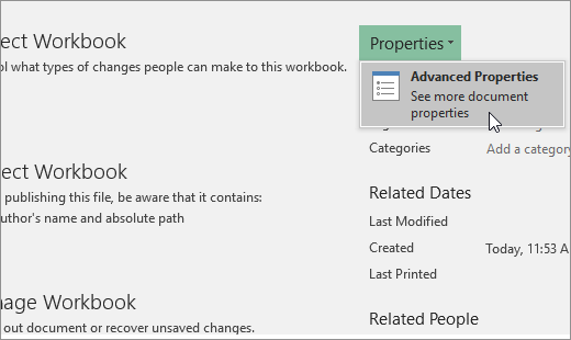
In Excel 2016, Excel 2013, and Excel 2010:
-
Click the File tab.
-
Click Info.
-
Click Properties, and then select Advanced Properties.
-
In the Summary tab, in the Hyperlink base text box, type the path that you want to use.
Note: You can override the link base address by using the full, or absolute, address for the link in the Insert Hyperlink dialog box.
-
-
In Excel 2007:
-
Click the Microsoft Office Button
, click Prepare, and then click Properties. -
In the Document Information Panel, click Properties, and then click Advanced Properties.
-
Click the Summary tab.
-
In the Hyperlink base box, type the path that you want to use.
Note: You can override the link base address by using the full, or absolute, address for the link in the Insert Hyperlink dialog box.
-
 , click Prepare, and then click Properties.
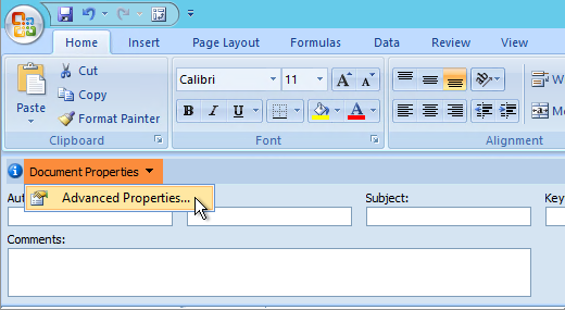
To delete a link, do one of the following:
-
To delete a link and the text that represents it, right-click the cell that contains the link, and then click Clear Contents on the shortcut menu.
-
To delete a link and the graphic that represents it, hold down Ctrl and click the graphic, and then press Delete.
-
To turn off a single link, right-click the link, and then click Remove Link on the shortcut menu.
-
To turn off several links at once, do the following:
-
In a blank cell, type the number 1.
-
Right-click the cell, and then click Copy on the shortcut menu.
-
Hold down Ctrl and select each link that you want to turn off.
Tip: To select a cell that has a link in it without going to the link destination, click the cell and hold the mouse button until the pointer becomes a cross
, and then release the mouse button. -
On the Home tab, in the Clipboard group, click the arrow below Paste, and then click Paste Special.
-
Under Operation, click Multiply, and then click OK.
-
On the Home tab, in the Styles group, click Cell Styles.
-
Under Good, Bad, and Neutral, select Normal.
-
A link opens another page or file when you click it. The destination is frequently another web page, but it can also be a picture, or an email address, or a program. The link itself can be text or a picture.
When a site user clicks the link, the destination is shown in a Web browser, opened, or run, depending on the type of destination. For example, a link to a page shows the page in the web browser, and a link to an AVI file opens the file in a media player.
How links are used
You can use links to do the following:
-
Navigate to a file or web page on a network, intranet, or Internet
-
Navigate to a file or web page that you plan to create in the future
-
Send an email message
-
Start a file transfer, such as downloading or an FTP process
When you point to text or a picture that contains a link, the pointer becomes a hand  , indicating that the text or picture is something that you can click.
What a URL is and how it works
When you create a link, its destination is encoded as a Uniform Resource Locator (URL), such as:
http://example.microsoft.com/news.htm
file://ComputerName/SharedFolder/FileName.htm
A URL contains a protocol, such as HTTP, FTP, or FILE, a Web server or network location, and a path and file name. The following illustration defines the parts of the URL:
1. Protocol used (http, ftp, file)
2. Web server or network location
3. Path
4. File name
Absolute and relative links
An absolute URL contains a full address, including the protocol, the Web server, and the path and file name.
A relative URL has one or more missing parts. The missing information is taken from the page that contains the URL. For example, if the protocol and web server are missing, the web browser uses the protocol and domain, such as .com, .org, or .edu, of the current page.
It is common for pages on the web to use relative URLs that contain only a partial path and file name. If the files are moved to another server, any links will continue to work as long as the relative positions of the pages remain unchanged. For example, a link on Products.htm points to a page named apple.htm in a folder named Food; if both pages are moved to a folder named Food on a different server, the URL in the link will still be correct.
In an Excel workbook, unspecified paths to link destination files are by default relative to the location of the active workbook. You can set a different base address to use by default so that each time that you create a link to a file in that location, you only have to specify the file name, not the path, in the Insert Hyperlink dialog box.
-
On a worksheet, select the cell where you want to create a link.
-
On the Insert tab, select Hyperlink.
You can also right-click the cell and then select Hyperlink… on the shortcut menu, or you can press Ctrl+K.
-
Under Display Text:, type the text that you want to use to represent the link.
-
Under URL:, type the complete Uniform Resource Locator (URL) of the webpage you want to link to.
-
Select OK.
To link to a location in the current workbook, you can either define a name for the destination cells or use a cell reference.
-
To use a name, you must name the destination cells in the workbook.
How to define a name for a cell or a range of cells
Note: In Excel for the Web, you can’t create named ranges. You can only select an existing named range from the Named Ranges control. Alternately, you can open the file in the Excel desktop app, create a named range there, and then access this option from Excel for the web.
-
Select the cell or range of cells that you want to name.
-
On the Name Box box at the left end of the formula bar
, type the name for the cells, and then press Enter.Note: Names can’t contain spaces and must begin with a letter.
-
-
On the worksheet, select the cell where you want to create a link.
-
On the Insert tab, select Hyperlink.
You can also right-click the cell and then select Hyperlink… on the shortcut menu, or you can press Ctrl+K.
-
Under Display Text:, type the text that you want to use to represent the link.
-
Under Place in this document:, enter the defined name or cell reference.
-
Select OK.
When you click a link to an email address, your email program automatically starts and creates an email message with the correct address in the To box, provided that you have an email program installed.
-
On a worksheet, select the cell where you want to create a link.
-
On the Insert tab, select Hyperlink.
You can also right-click the cell and then select Hyperlink… on the shortcut menu, or you can press Ctrl+K.
-
Under Display Text:, type the text that you want to use to represent the link.
-
Under E-mail address:, type the email address that you want.
-
Select OK.
You can also create a link to an email address in a cell by typing the address directly in the cell. For example, a link is created automatically when you type an email address, such as someone@example.com.
You can use the HYPERLINK function to create a link to a URL.
Note: The Link_location can be a text string enclosed in quotation marks or a reference to a cell that contains the link as a text string.
To select a hyperlink without activating the link to its destination, do any of the following:
-
Select a cell by clicking it when the pointer is an arrow.
-
Use the arrow keys to select the cell that contains the link.
You can change an existing link in your workbook by changing its destination, its appearance, or the text that is used to represent it.
-
Select the cell that contains the link that you want to change.
Tip: To select a hyperlink without activating the link to its destination, use the arrow keys to select the cell that contains the link.
-
On the Insert tab, select Hyperlink.
You can also right-click the cell or graphic and then select Edit Hyperlink… on the shortcut menu, or you can press Ctrl+K.
-
In the Edit Hyperlink dialog box, make the changes that you want.
Note: If the link was created by using the HYPERLINK worksheet function, you must edit the formula to change the destination. Select the cell that contains the link, and then select the formula bar to edit the formula.
-
Right-click the hyperlink that you want to copy or move, and then select Copy or Cut on the shortcut menu.
-
Right-click the cell that you want to copy or move the link to, and then select Paste on the shortcut menu.
To delete a link, do one of the following:
-
To delete a link, select the cell and press Delete.
-
To turn off a link (delete the link but keep the text that represents it), right-click the cell and then select Remove Hyperlink.
Need more help?
You can always ask an expert in the Excel Tech Community or get support in the Answers community.
See Also
Remove or turn off links
See all How-To Articles
This tutorial demonstrates how to hyperlink to another sheet or workbook in Excel and Google Sheets.
Link to Another Sheet
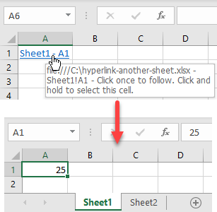
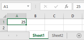
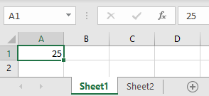
In Excel, you can create a hyperlink to a cell in another sheet. Say you have value 25 in cell A1 of Sheet1 and want to create a hyperlink to this cell in Sheet2.
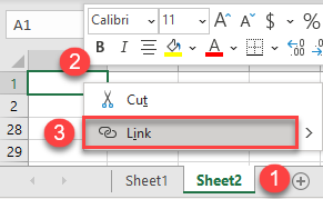
- Go to another sheet (Sheet2), right-click the cell where you want to insert a hyperlink (A1), and click Link.
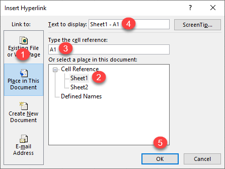
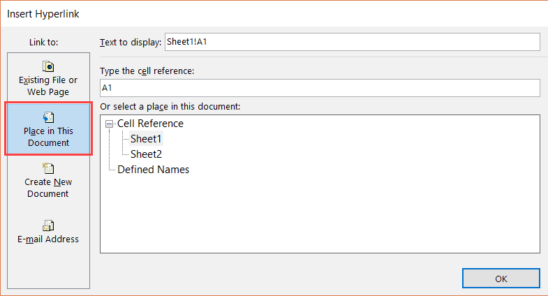
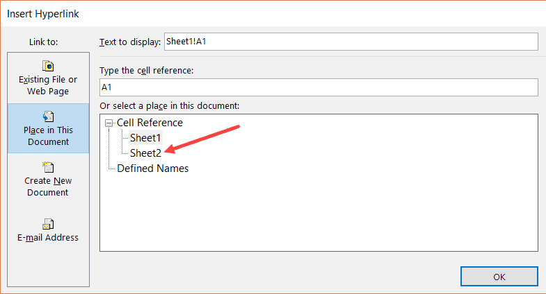
- In the Insert Hyperlink window, (1) select Place in This Document, (2) choose a sheet to which you want to link (Sheet1), (3) enter the cell you want to link to (A1), (4) enter text to display in the linked cell (Sheet1 – A1), and (5) click OK.
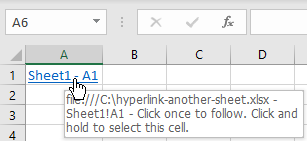
As a result, the hyperlink is inserted in cell A1 of Sheet2. By default, the text of the hyperlink is underlined and colored in blue. If you position a mouse cursor over the hyperlink, you can see the file destination and name, as well as a cell that it’s leading to.
And when you click on the hyperlink, you’ll be redirected to the linked cell.
The HYPERLINK Function
Another way to insert a hyperlink to another sheet is to use the HYPERLINK Function. Enter this formula in cell A1 of Sheet2:
=HYPERLINK(Sheet1!A1,"Sheet1 - A1")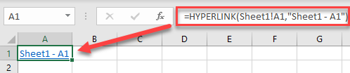
The first argument of the function is the cell to which you want to navigate the link, and the second argument is the text that is displayed in the link. The result is the same as using the previous method.
Hyperlink to Another Workbook
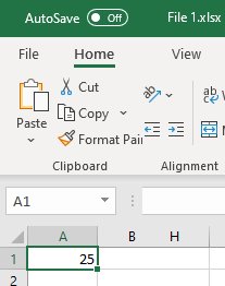
You can also insert a hyperlink to another workbook. Say that in File 1.xlsx you have a value of 25 in cell A1 and want to link it to File 2.xlsx.

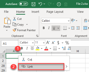
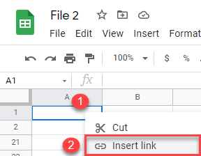
- In File 2.xlsx, right-click the cell where you want to insert a hyperlink (A1) and click Link.
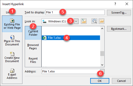
- In the Insert Hyperlink window, (1) select Existing File or Web Page, (2) choose Current Folder – or (3) select the folder with your source file – and (4) select the file (File 1.xlsx). (5) Enter text to display in the linked cell (File 1), and (6) click OK.
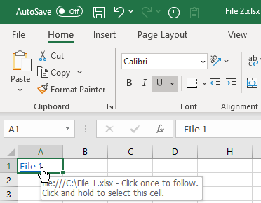
As a result, the hyperlink to File 1.xlsx is inserted into cell A1 of File 2.xlsx. If you position a mouse cursor over this cell, you can see the linked file destination and name.
If you click on the link, you’re redirected to cell A1 of the source file. If the source file is not opened, it is opened once you click the hyperlink.
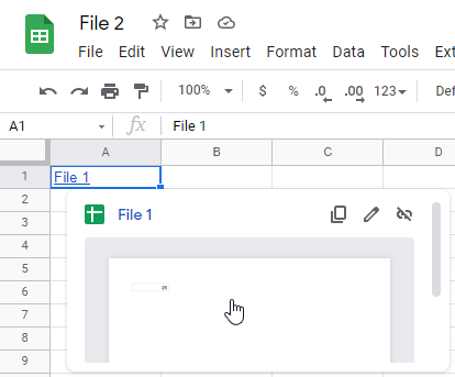
Link to Another Google Sheets Tab
To create a hyperlink to another sheet in Google Sheets, follow these steps:
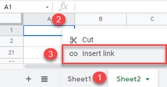
- Go to another sheet (Sheet2), right-click the cell where you want to insert a hyperlink (A1), and click Insert link.
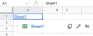
- Select the sheet you want to link to (Sheet1).
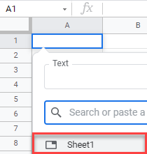
As a result, the hyperlink is inserted in cell A1 of Sheet2. By default, the text of the hyperlink is underlined and colored in blue. If you click on a cell with the link, you can see the linked sheet.
And when you click on the hyperlink, you’ll be redirected to the linked sheet.
Link to Another Google Sheet
Say you have File 1 in Google Sheets with value 25 in cell A1 and want to link this cell to File 2.
- Right-click the URL address of the source file (File 1) and click Copy.
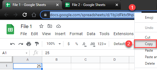
- Now go to another file (File 2), right-click the cell where you want to insert a hyperlink (A1), and click Insert link.
- Paste the copied link, enter text to display, and click Apply.

As a result, the hyperlink is inserted in cell A1. If you click on this cell, you can navigate to the linked file (File 1).
Note: You can also use the HYPERLINK Function in Google Sheets, same as in Excel. The only difference is that for Google Sheets, you have to enter the URL.
Skip to content
В статье разъясняется, как сделать гиперссылку в Excel, используя 3 разных метода. Вы узнаете, как вставлять, изменять и удалять гиперссылки на рабочих листах, а также исправлять неработающие ссылки.
Гиперссылки широко используются в Интернете для навигации между веб-сайтами.
Если вы настоящий интернет-серфер, вы не понаслышке знаете о пользе гиперссылок. Щелкая по ним, вы моментально получаете доступ к другой информации, где бы она ни находилась. Но знаете ли вы о том, как можно использовать гиперссылки в таблицах Excel? Пришло время разобраться и начать использовать эту функцию Excel.
В ваших таблицах Excel вы можете легко создавать такие ссылки. Кроме того, вы можете вставить гиперссылку, чтобы перейти к другой ячейке, листу или книге, открыть новый файл Excel или создать сообщение электронной почты. В этом руководстве представлены подробные инструкции о том, как это сделать в Excel 365, 2019, 2016, 2013, 2010 и более ранних версиях.
Что такое гиперссылка в Excel
Гиперссылка Excel — это ссылка на определенное место, документ или веб-страницу, на которую пользователь может перейти, кликнув по ней.
Microsoft Excel позволяет создавать гиперссылки для различных целей, включая:
- Переход к определенному месту в текущей рабочей книге
- Открытие другого документа или переход к определенному месту в этом документе, например листу в файле Excel или закладке в документе Word
- Переход на веб-страницу в Интернете
- Создание нового файла Excel
- Отправка письма на указанный адрес
Гиперссылки в Excel легко узнаваемы — обычно это текст, выделенный подчеркиванием и синим цветом.
В Microsoft Excel одну и ту же задачу часто можно выполнить несколькими различными способами, и это также верно для создания гиперссылок. Чтобы создать гиперссылку в Excel, вы можете использовать любой из следующих способов:
- Диалоговое окно «Вставить гиперссылку»
- Функция ГИПЕРССЫЛКА
- код VBA
Как создать гиперссылку с помощью диалогового окна
Самый распространенный способ поместить гиперссылку непосредственно в ячейку — использовать диалоговое окно «Вставить гиперссылку», доступ к которому можно получить тремя различными способами. Просто выберите ячейку, в которую вы хотите вставить ссылку, и выполните одно из следующих действий:
- На вкладке меню «Вставка» в группе «Ссылки» нажмите кнопку «Гиперссылка» или «Ссылка» в зависимости от версии Excel.
- Щелкните ячейку правой кнопкой мыши и выберите «Гиперссылка…» ( «Ссылка» в последних версиях) в контекстном меню.

Рис 1.
- Нажмите комбинацию клавиш
Ctrl + К.
А теперь, в зависимости от того, какую ссылку вы хотите создать, перейдите к одному из следующих примеров:
- Гиперссылка на другой документ
- Гиперссылка на веб-страницу (URL)
- Гиперссылка на ячейку в текущей книге
- Гиперссылка на новую книгу
- Гиперссылка на адрес электронной почты
Гиперссылка на другой файл
Чтобы сделать гиперссылку, которая будет указывать на другой документ, например другой файл Excel, документ Word или презентацию PowerPoint, откройте диалоговое окно «Вставка гиперссылки» в Excel и выполните следующие действия:
- На левой панели в разделе «Связать с:» выберите «файлом или веб-страницей».
- В списке «Искать в» перейдите к нужному местоположению, а затем выберите сам файл.
- В поле «Текст» введите то, что должно отображаться в ячейке («Книга1» в этом примере). Если не вводить ничего, то по умолчанию будет отображаться имя выбранного ранее объекта.
- При необходимости нажмите кнопку «Подсказка…» в правом верхнем углу и введите текст, который будет отображаться, когда пользователь наводит указатель мыши на гиперссылку. В данном примере это может быть «Перейти к Книга1 в Гиперссылках».
- Нажмите «ОК».

Гиперссылка вставляется в выбранную ячейку и выглядит точно так, как вы ее настроили:

Чтобы сделать ссылку на определенный лист или ячейку, нажмите кнопку «Закладка…» в правой части диалогового окна «Вставка гиперссылки», затем выберите нужный рабочий лист и введите адрес целевой ячейки в поле «Введите адрес ячейки». Нажмите «ОК».

Чтобы создать ссылку на именованный диапазон, выберите его в списке Определенные имена, как показано ниже:

Добавить гиперссылку на веб-адрес (URL)
Чтобы сделать гиперссылку на сайт, откройте диалоговое окно «Вставка гиперссылки» и выполните следующие действия:
- В разделе «Связать с:» выберите «файлом или веб-страницей».
- Нажмите кнопку «Обзор Интернета», затем откройте сайт, на который вы хотите сослаться, переключитесь обратно в Excel, не закрывая веб-браузер.
Excel автоматически вставит адрес веб-сайта и текст для отображения. Вы можете изменить этот текст, чтобы он отображался так, как вы хотите. При необходимости введите всплывающую подсказку и нажмите «ОК», чтобы добавить созданную гиперссылку.

Кроме того, вы можете просто скопировать URL-адрес страницы сайта в буфер обмена, а потом открыть диалоговое окно «Вставка гиперссылки» и просто вставить URL-адрес в поле «Адрес».
Гиперссылка на лист или ячейку в текущей книге
Один из способов, как вы можете эффективно использовать гиперссылки электронных таблиц, — это создать оглавление вашей рабочей книги. Внутренние гиперссылки Excel помогут вам быстро перейти к нужной части книги, особенно если в ней много листов и больших таблиц.
Первый способ создания гиперссылки на лист внутри одной книги — использование команды «Гиперссылка».
- Выберите ячейку, в которую вы хотите вставить гиперссылку на ячейку или на файл.
- Щелкните правой кнопкой мыши ячейку и выберите пункт «Ссылка» в контекстном меню.
На экране появится диалоговое окно «Вставка гиперссылки». - Выберите «Место в документе» в разделе «Связать с», если ваша задача — связать ячейку с определенным местом в той же книге. Или же выберите нужный файл, как мы это уже делали ранее.
- Укажите рабочий лист, на который вы хотите сослаться, в поле Или выберите место в этом документе.
- Введите адрес ячейки в поле Введите ссылку на ячейку, если вы хотите указать на определенную ячейку другого рабочего листа. Получится гиперссылка на ячейку в Excel. Можно это не делать, тогда по ссылке просто откроется этот лист.
- Введите значение или имя в поле Текст, чтобы как-то назвать гиперссылку в ячейке.

- Нажмите ОК .

Текст в ячейке будет подчеркнут и выделен синим цветом. Это означает, что ячейка содержит гиперссылку. Чтобы проверить, работает ли она, просто наведите указатель мыши на этот подчеркнутый текст и щелкните по нему, чтобы перейти в указанное место.
Гиперссылка на другую книгу Excel
Помимо ссылки на существующие файлы, вы можете создать гиперссылку на новый файл Excel. Вот как:
- В разделе «Связать с» щелкните значок «Новый документ».
- В поле Текст введите текст ссылки, который будет отображаться в ячейке.
- В поле Имя нового документа введите новое имя книги, которую вы создадите.
- В поле Адрес проверьте место, где будет сохранен созданный файл. Если вы хотите изменить расположение по умолчанию, нажмите кнопку Изменить.
- В разделе Когда вносить правку выберите нужный вариант редактирования.
- Нажмите ОК .

Гиперссылка для создания сообщения электронной почты
Помимо ссылок на различные документы, функция гиперссылки Excel позволяет отправлять сообщения электронной почты прямо с рабочего листа. Чтобы это сделать, выполните следующие действия:
- В разделе «Связать с» выберите значок «Электронная почта».
- В поле Адрес электронной почты введите адрес почты получателя или несколько адресов, разделенных точкой с запятой. Кстати, «mailto:» вводить не нужно, Excel сам подставит этот префикс.
- При желании введите тему сообщения в поле Тема. Имейте в виду, что некоторые браузеры и почтовые клиенты могут не распознавать строку темы.
- В поле Текст введите нужный текст ссылки.
- При необходимости нажмите кнопку «Подсказка…» и введите нужный текст (подсказка будет отображаться при наведении указателя мыши на гиперссылку).
- Нажмите «ОК».

Совет. Самый быстрый способ сделать гиперссылку на конкретный адрес электронной почты — это набрать адрес электронной почты прямо в ячейке на вашем рабочем листе. Как только вы нажмете клавишу Enter, Excel автоматически преобразует его в интерактивную гиперссылку.
Как создавать ссылки с помощью формулы ГИПЕРССЫЛКА
Если вы один из тех профессионалов Excel, которые используют формулы для решения большинства задач, вы можете использовать функцию ГИПЕРССЫЛКА, которая специально разработана для вставки гиперссылок в Excel. Это особенно полезно, когда вы собираетесь создавать, редактировать или удалять несколько ссылок одновременно.
Синтаксис формулы ГИПЕРССЫЛКА следующий:
ГИПЕРССЫЛКА( адрес ; [имя] )
Где:
- адрес — это путь к целевому документу или веб-странице.
- имя — это текст ссылки, который будет отображаться в ячейке.
Например, чтобы сделать гиперссылку с названием «Исходные данные», которая открывает Лист2 в книге с именем «Исходные данные», хранящейся в папке «Файлы Excel» на диске D, используйте следующую формулу:
=ГИПЕРССЫЛКА(«[D:Excel filesИсходные данные.xlsx]Лист2!A1»; «Исходные данные»)
Подробное объяснение аргументов функции ГИПЕРССЫЛКА и примеры формул для создания различных типов ссылок см. в статье Как использовать функцию гиперссылки в Excel .
Вставьте ссылку, перетащив ячейку
Самый быстрый способ создания гиперссылок внутри одной книги — использование метода перетаскивания. Позвольте мне показать вам, как это работает.
В качестве примера я возьму книгу из двух листов и создам гиперссылку на листе 1, которая ведёт на ячейку на листе 2.
Примечание. Убедитесь, что книга сохранена, потому что этот метод не работает в новых книгах.
- Выберите ячейку назначения гиперссылки на листе 2.
- Наведите указатель мыши на одну из границ ячейки и щелкните правой кнопкой мыши.

- Удерживая правую кнопку, переместите указатель мыши к вкладкам листов.

- Нажмите клавишу
ALTи наведите указатель мыши на вкладку Лист 1.Нажатая клавиша
ALTпозволит переместиться на другой лист. Как только лист 1 активирован, вы можете перестать удерживать клавишу. - Продолжайте перетаскивать курсор мыши в то место, куда вы хотите вставить гиперссылку.

- Отпустите правую кнопку мыши, чтобы появилось всплывающее меню.
- Выберите «Создать гиперссылку».

После этого в ячейке появится гиперссылка. Когда вы нажмете на нее, вы сразу переместитесь на ячейку назначения на листе 2.
Без сомнения, перетаскивание — самый быстрый способ вставить гиперссылку на лист Excel. Он объединяет несколько операций в одно действие. Это займет у вас меньше времени, но немного больше концентрации внимания, чем два других метода. Так что вам решать, каким путем
лучше идти.
Как вставить гиперссылку в Excel с помощью VBA
Чтобы автоматизировать создание гиперссылки на ваших листах, вы можете использовать этот простой код VBA:
Public Sub AddHyperlink()

  Sheets("Sheet1").Hyperlinks.Add Anchor:=Sheets("Sheet1").Range("A1"), Address:="", SubAddress:="Sheet3!B5", TextToDisplay:="My hyperlink"

End Sub
Где:
- Sheets — имя листа, на который должна быть вставлена ссылка (в данном примере Sheet1).
- Range — ячейка, в которую следует вставить ссылку (в данном примере A1).
- SubAddress — место назначения ссылки, т.е. куда должна указывать гиперссылка (в данном примере Sheet3!B5).
- TextToDisplay — текст, который будет отображаться в ячейке (в данном примере — «Моя гиперссылка»).
Этот макрос вставит гиперссылку под названием «Моя гиперссылка» в ячейку A1 на листе Sheet1 в активной книге. Нажав на ссылку, вы перейдете к ячейке B5 на листе 3 в той же книге.
Как открыть и изменить гиперссылку в Excel
Вы можете изменить существующую гиперссылку в своей книге, изменив ее назначение, внешний вид или текст, используемый для ее представления.
Поскольку в этой статье речь идет о гиперссылках между электронными таблицами одной и той же книги, назначением гиперссылки в этом случае является определённая ячейка из другой электронной таблицы. Если вы хотите изменить место назначения гиперссылки, вам нужно изменить ссылку на ячейку или выбрать другой лист. Вы можете сделать и то, и другое, если это необходимо.
- Щелкните правой кнопкой мыши гиперссылку, которую хотите изменить.
- Выберите «Редактировать гиперссылку» во всплывающем меню.

На экране появится диалоговое окно «Изменение гиперссылки». Вы видите, что оно выглядит точно так же, как диалоговое окно «Вставка гиперссылки», и имеет те же поля.

Примечание. Есть еще как минимум два способа открыть гиперссылку. Вы можете нажать комбинацию Ctrl + К или кнопку «Гиперссылка» в группе «Ссылки» на вкладке меню «ВСТАВКА». Но не забудьте перед этим выделить нужную ячейку.
- Обновите информацию в соответствующих полях диалогового окна «Изменение гиперссылки».
- Нажмите «ОК» и проверьте, куда сейчас ведёт гиперссылка.
Примечание. Если вы использовали формулу для добавления гиперссылки в Excel, вам необходимо открыть и отредактировать её, чтобы изменить место назначения. Выберите ячейку, содержащую ссылку, и поместите курсор в строку формул, чтобы отредактировать.
Здесь у вас могут возникнуть некоторые сложности. Мы привыкли, что для того, чтобы открыть и внести изменения в содержимое ячейки, достаточно кликнуть на ней мышкой, чтобы перейти в режим редактирования.
Кликнув ячейку, содержащую гиперссылку, вы не откроете её, а перейдете к месту назначения ссылки, т. е. к целевому документу или веб-странице. Чтобы выбрать для редактирования ячейку, не переходя к расположению ссылки, щелкните ячейку и удерживайте кнопку мыши, пока указатель не превратится в крестик (курсор выбора Excel), а уж затем отпустите кнопку.

Если гиперссылка занимает только часть ячейки (т. е. если ваша ячейка шире текста ссылки), наведите указатель мыши на пустое место, и как только он изменится с указывающей руки на крест, щелкните ячейку:

Еще один способ выбрать ячейку без открытия гиперссылки — выбрать соседнюю ячейку и с помощью клавиш со стрелками установить курсор на ячейке со ссылкой.
Чтобы изменить сразу несколько формул гиперссылок, используйте функцию Excel «Заменить все», как показано в этом совете.
Как изменить внешний вид гиперссылки
Чаще всего гиперссылки отображаются в виде подчеркнутого текста синего цвета. Если типичный вид текста гиперссылки кажется вам скучным и вы хотите выделиться из толпы, читайте ниже, как это сделать:
- Перейдите в группу Стили на вкладке ГЛАВНАЯ .
- Откройте список «Стили ячеек».
- Щелкните правой кнопкой мыши на кнопке «Гиперссылка», чтобы изменить внешний вид. Или щелкните правой кнопкой мыши на «Открывавшаяся гиперссылка», если нужно изменить вид ссылок, по которым уже переходили.
- Выберите опцию «Изменить» в контекстном меню.

- Нажмите «Формат» в диалоговом окне «Стили».
- Внесите необходимые изменения в диалоговом окне «Формат ячеек». Здесь вы можете изменить выравнивание и шрифт гиперссылки или добавить цвет заливки.
- Когда вы закончите, нажмите OK.
- Убедитесь, что все изменения отмечены в разделе «Стиль включает» в диалоговом окне «Стиль».
- Нажмите ОК.
Теперь вы можете наслаждаться новым индивидуальным стилем гиперссылок в своей книге. Обратите внимание, что внесенные вами изменения влияют на все гиперссылки в текущей книге. Вы не можете изменить внешний вид только одной гиперссылки.
Как убрать гиперссылку в Excel
Удаление гиперссылок в Excel выполняется в два клика. Вы просто щелкаете ссылку правой кнопкой мыши и выбираете «Удалить гиперссылку» в контекстном меню.

Это удалит интерактивную гиперссылку, но сохранит текст ссылки в ячейке. То есть, гиперссылка превратится в текст. Чтобы также удалить текст ссылки, щелкните ячейку правой кнопкой мыши и выберите «Очистить содержимое» .
Совет. Чтобы удалить сразу все или несколько выбранных гиперссылок, используйте функцию «Специальная вставка», как показано в статье «Как удалить несколько гиперссылок в Excel». Также там описаны и другие способы удаления.
Как извлечь веб-адрес (URL) из гиперссылки Excel
Есть два способа извлечь URL-адрес из гиперссылки в Excel: вручную и программно.
Извлечь URL-адрес из гиперссылки вручную
Если у вас всего пара гиперссылок, вы можете быстро извлечь их назначения, выполнив следующие простые шаги:
- Выберите ячейку, содержащую гиперссылку.
- Откройте диалоговое окно «Редактировать гиперссылку», нажав
Ctrl + Кили щелкните гиперссылку правой кнопкой мыши и выберите «Редактировать гиперссылку». - В поле Адрес выберите URL-адрес и нажмите
Ctrl + С, чтобы скопировать его.

- Нажмите Esc или OK, чтобы закрыть окно редактирования.
- Вставьте скопированный URL-адрес в любую пустую ячейку. Готово!
Извлечение нескольких URL-адресов с помощью VBA
Если у вас много гиперссылок на листах Excel, извлечение каждого URL-адреса вручную было бы весьма утомительной тратой времени.
Предлагаемый ниже макрос может ускорить процесс, автоматически извлекая адреса из всех гиперссылок на текущем листе:
Sub ExtractHL()
  Dim HL As Hyperlink
  Dim OverwriteAll As Boolean

  OverwriteAll = False

  For Each HL In ActiveSheet.Hyperlinks

    If Not OverwriteAll Then
        If HL.Range.Offset(0, 1).Value <> "" Then
            If MsgBox("One or more of the target cells is not empty. Do you want to overwrite all cells?", vbOKCancel, "Target cells are not empty") = vbCancel Then
                Exit For
            Else
                OverwriteAll = True
            End If
        End If
    End If
    HL.Range.Offset(0, 1).Value = HL.Address
  Next

End Sub
Как показано на скриншоте ниже, код VBA получает URL-адреса из столбца гиперссылок и помещает результаты в соседние ячейки.

Если одна или несколько ячеек в соседнем столбце содержат данные, код отобразит диалоговое окно с предупреждением, спрашивающее пользователя, хотят ли они перезаписать текущие данные.
Преобразование объектов рабочего листа в гиперссылки
Преобразовать можно не только текст в гиперссылку. Многие объекты рабочего листа, включая диаграммы, изображения, текстовые поля и фигуры, также можно превратить в интерактивные гиперссылки. Для этого достаточно щелкнуть объект правой кнопкой мыши (как, например, объект WordArt на скриншоте ниже), нажать «Гиперссылка…» и настроить ссылку, как описано в разделе «Как создать гиперссылку в Excel» .

Совет. Меню диаграмм, вызываемое правой кнопкой мыши, не имеет параметра «Гиперссылка». Чтобы преобразовать диаграмму Excel в гиперссылку, выберите диаграмму и нажмите Ctrl + К.
Не открывается гиперссылка в Excel — причины и решения
Если гиперссылки не работают должным образом на ваших листах, следующие шаги по устранению неполадок помогут вам определить источник проблемы и устранить ее.
Ссылка недействительна
Симптомы: щелчок по гиперссылке в Excel не приводит пользователя к месту назначения, а выдает ошибку «Ссылка недействительна».
Решение . Когда вы создаете гиперссылку на другой лист, имя листа становится целью ссылки. Если вы позже переименуете этот рабочий лист, Excel не сможет найти цель, и гиперссылка перестанет работать. Чтобы исправить это, вам нужно либо изменить имя листа обратно на исходное имя, либо отредактировать гиперссылку, чтобы она указывала на переименованный лист.
Если вы создали гиперссылку на другой файл, а затем переместили этот файл в другое место, вам нужно будет указать новый путь к файлу.
Гиперссылка отображается как обычная текстовая строка
Симптомы . Набранные, скопированные или импортированные на лист web-адреса (URL-адреса) не преобразуются автоматически в интерактивные гиперссылки и не выделяются традиционным подчеркнутым синим форматированием. Или же гиперссылка не активна, хоть и выглядят нормально. Ничего не происходит, когда вы нажимаете на нее.
Решение . Дважды щелкните ячейку или нажмите F2, чтобы войти в режим редактирования, затем перейдите в конец URL-адреса и нажмите клавишу пробела. Excel преобразует текстовую строку в интерактивную гиперссылку. Если таких ссылок много, проверьте формат своих ячеек. Иногда возникают проблемы со ссылками, размещенными в ячейках с общим форматом. В этом случае попробуйте изменить формат ячейки на Текст.
Гиперссылки перестали работать после повторного открытия книги
Симптомы. Гиперссылки Excel работали нормально, пока вы не сохранили и не открыли книгу заново. Теперь они все серые и больше не работают.
Решение : Прежде всего, проверьте, не было ли изменено место назначения ссылки, то есть целевой документ не был ни переименован, ни перемещен. Если это не так, вы можете отключить параметр, который заставляет Excel проверять гиперссылки при каждом сохранении книги. Были сообщения о том, что Excel иногда отключает нормально работающие гиперссылки. Например, ссылки на файлы, хранящиеся в вашей локальной сети, могут быть отключены из-за некоторых временных проблем с вашим сервером. Или ссылки на URL-адреса будут отключены при временном пропадании интернета. Чтобы отключить этот параметр, выполните следующие действия:
- В Excel 2010 и новее щелкните Файл > Параметры. В Excel 2007 нажмите кнопку Office > Параметры Excel.
- На левой панели выберите «Дополнительно».
- Прокрутите вниз до раздела «Общие» и нажмите «Параметры Интернета…».
- В диалоговом окне «Параметры веб-документа» перейдите на вкладку «Файлы», снимите флажок «Обновлять ссылки при сохранении» и нажмите «ОК» .

Гиперссылки на основе формул не работают
Симптомы. Ссылка, созданная с помощью функции ГИПЕРССЫЛКА, не открывается или в ячейке отображается значение ошибки.
Решение. Большинство проблем с гиперссылками на основе формул вызваны несуществующим или неправильным путем, указанным в аргументе адрес. Перейдите по ссылкам ниже, чтобы узнать, как правильно создать формулу гиперссылки. Дополнительные шаги по устранению неполадок см. в разделе Функция Excel ГИПЕРССЫЛКА не работает.
Вот как вы можете создавать, редактировать и удалять гиперссылки в Excel. Благодарю вас за чтение.
Другие статьи по теме:
Содержание
- Hyperlink to Another Sheet or Workbook in Excel & Google Sheets
- Link to Another Sheet
- The HYPERLINK Function
- Hyperlink to Another Workbook
- Link to Another Google Sheets Tab
- Link to Another Google Sheet
- HYPERLINK function
- Description
- Syntax
- Remark
- Examples
- Hyperlinks in Excel (A Complete Guide + Examples)
- How to Insert Hyperlinks in Excel
- Manually Type the URL
- Insert Using the Dialog Box
- Insert Using the HYPERLINK Function
- Create a Hyperlink to a Worksheet in the Same Workbook
- Create a Hyperlink to a File (in the same or different folders)
- Create a Hyperlink to a Folder
- Create Hyperlink to an Email Address
- Remove Hyperlinks
- Manually Remove Hyperlinks
- Remove Hyperlinks Using VBA
- Prevent Excel from Creating Hyperlinks Automatically
- Extract Hyperlink URLs (using VBA)
- Extract Hyperlink in the Adjacent Column
- Extract Hyperlink Using a Formula (created with VBA)
- Find Hyperlinks with Specific Text
- Selecting a Cell that has a Hyperlink in Excel
- Select the Cell (without opening the URL)
- Select a Cell by clicking on the blank space in the cell
- Some Practical Example of Using Hyperlink
- Example 1 – Create an Index of All Sheets in the Workbook
- Example 2 – Create Dynamic Hyperlinks
- Example 3 – Quickly Generate Simple Emails Using Hyperlink Function
Hyperlink to Another Sheet or Workbook in Excel & Google Sheets
This tutorial demonstrates how to hyperlink to another sheet or workbook in Excel and Google Sheets.
Link to Another Sheet
In Excel, you can create a hyperlink to a cell in another sheet. Say you have value 25 in cell A1 of Sheet1 and want to create a hyperlink to this cell in Sheet2.
- Go to another sheet (Sheet2), right-click the cell where you want to insert a hyperlink (A1), and click Link.
- In the Insert Hyperlink window, (1) select Place in This Document, (2) choose a sheet to which you want to link (Sheet1), (3) enter the cell you want to link to (A1), (4) enter text to display in the linked cell (Sheet1 – A1), and (5) click OK.
As a result, the hyperlink is inserted in cell A1 of Sheet2. By default, the text of the hyperlink is underlined and colored in blue. If you position a mouse cursor over the hyperlink, you can see the file destination and name, as well as a cell that it’s leading to.
And when you click on the hyperlink, you’ll be redirected to the linked cell.
The HYPERLINK Function
Another way to insert a hyperlink to another sheet is to use the HYPERLINK Function. Enter this formula in cell A1 of Sheet2:
The first argument of the function is the cell to which you want to navigate the link, and the second argument is the text that is displayed in the link. The result is the same as using the previous method.
Hyperlink to Another Workbook
You can also insert a hyperlink to another workbook. Say that in File 1.xlsx you have a value of 25 in cell A1 and want to link it to File 2.xlsx.
- In File 2.xlsx, right-click the cell where you want to insert a hyperlink (A1) and click Link.
- In the Insert Hyperlink window, (1) select Existing File or Web Page, (2) choose Current Folder – or (3) select the folder with your source file – and (4) select the file (File 1.xlsx). (5) Enter text to display in the linked cell (File 1), and (6) click OK.
As a result, the hyperlink to File 1.xlsx is inserted into cell A1 of File 2.xlsx. If you position a mouse cursor over this cell, you can see the linked file destination and name.
If you click on the link, you’re redirected to cell A1 of the source file. If the source file is not opened, it is opened once you click the hyperlink.
Link to Another Google Sheets Tab
To create a hyperlink to another sheet in Google Sheets, follow these steps:
- Go to another sheet (Sheet2), right-click the cell where you want to insert a hyperlink (A1), and click Insert link.
- Select the sheet you want to link to (Sheet1).
As a result, the hyperlink is inserted in cell A1 of Sheet2. By default, the text of the hyperlink is underlined and colored in blue. If you click on a cell with the link, you can see the linked sheet.
And when you click on the hyperlink, you’ll be redirected to the linked sheet.
Link to Another Google Sheet
Say you have File 1 in Google Sheets with value 25 in cell A1 and want to link this cell to File 2.
- Right-click the URL address of the source file (File 1) and click Copy.
- Now go to another file (File 2), right-click the cell where you want to insert a hyperlink (A1), and click Insert link.
- Paste the copied link, enter text to display, and click Apply.
As a result, the hyperlink is inserted in cell A1. If you click on this cell, you can navigate to the linked file (File 1).
Note: You can also use the HYPERLINK Function in Google Sheets, same as in Excel. The only difference is that for Google Sheets, you have to enter the URL.
Источник
HYPERLINK function
This article describes the formula syntax and usage of the HYPERLINK function in Microsoft Excel.
Description
The HYPERLINK function creates a shortcut that jumps to another location in the current workbook, or opens a document stored on a network server, an intranet, or the Internet. When you click a cell that contains a HYPERLINK function, Excel jumps to the location listed, or opens the document you specified.
Syntax
The HYPERLINK function syntax has the following arguments:
Link_location Required. The path and file name to the document to be opened. Link_location can refer to a place in a document — such as a specific cell or named range in an Excel worksheet or workbook, or to a bookmark in a Microsoft Word document. The path can be to a file that is stored on a hard disk drive. The path can also be a universal naming convention (UNC) path on a server (in Microsoft Excel for Windows) or a Uniform Resource Locator (URL) path on the Internet or an intranet.
Note Excel for the web the HYPERLINK function is valid for web addresses (URLs) only. Link_location can be a text string enclosed in quotation marks or a reference to a cell that contains the link as a text string.
If the jump specified in link_location does not exist or cannot be navigated, an error appears when you click the cell.
Friendly_name Optional. The jump text or numeric value that is displayed in the cell. Friendly_name is displayed in blue and is underlined. If friendly_name is omitted, the cell displays the link_location as the jump text.
Friendly_name can be a value, a text string, a name, or a cell that contains the jump text or value.
If friendly_name returns an error value (for example, #VALUE!), the cell displays the error instead of the jump text.
In the Excel desktop application, to select a cell that contains a hyperlink without jumping to the hyperlink destination, click the cell and hold the mouse button until the pointer becomes a cross  , then release the mouse button. In Excel for the web, select a cell by clicking it when the pointer is an arrow; jump to the hyperlink destination by clicking when the pointer is a pointing hand.
Examples
=HYPERLINK(«http://example.microsoft.com/report/budget report.xlsx», «Click for report»)
Opens a workbook saved at http://example.microsoft.com/report. The cell displays «Click for report» as its jump text.
=HYPERLINK(«[http://example.microsoft.com/report/budget report.xlsx]Annual!F10», D1)
Creates a hyperlink to cell F10 on the Annual worksheet in the workbook saved at http://example.microsoft.com/report. The cell on the worksheet that contains the hyperlink displays the contents of cell D1 as its jump text.
=HYPERLINK(«[http://example.microsoft.com/report/budget report.xlsx]’First Quarter’!DeptTotal», «Click to see First Quarter Department Total»)
Creates a hyperlink to the range named DeptTotal on the First Quarter worksheet in the workbook saved at http://example.microsoft.com/report. The cell on the worksheet that contains the hyperlink displays «Click to see First Quarter Department Total» as its jump text.
=HYPERLINK(«http://example.microsoft.com/Annual Report.docx]QrtlyProfits», «Quarterly Profit Report»)
To create a hyperlink to a specific location in a Word file, you use a bookmark to define the location you want to jump to in the file. This example creates a hyperlink to the bookmark QrtlyProfits in the file Annual Report.doc saved at http://example.microsoft.com.
Displays the contents of cell D5 as the jump text in the cell and opens the workbook saved on the FINANCE server in the Statements share. This example uses a UNC path.
Opens the workbook 1stqtr.xlsx that is stored in the Finance directory on drive D, and displays the numeric value that is stored in cell H10.
Creates a hyperlink to the Totals area in another (external) workbook, Mybook.xlsx.
=HYPERLINK(«[Book1.xlsx]Sheet1!A10″,»Go to Sheet1 > A10»)
To jump to a different location in the current worksheet, include both the workbook name, and worksheet name like this, where Sheet1 is the current worksheet.
=HYPERLINK(«[Book1.xlsx]January!A10″,»Go to January > A10»)
To jump to a different location in the current worksheet, include both the workbook name, and worksheet name like this, where January is another worksheet in the workbook.
=HYPERLINK(CELL(«address»,January!A1),»Go to January > A1″)
To jump to a different location in the current worksheet without using the fully qualified worksheet reference ([Book1.xlsx]), you can use this, where CELL(«address») returns the current workbook name.
To quickly update all formulas in a worksheet that use a HYPERLINK function with the same arguments, you can place the link target in another cell on the same or another worksheet, and then use an absolute reference to that cell as the link_location in the HYPERLINK formulas. Changes that you make to the link target are immediately reflected in the HYPERLINK formulas.
Источник
Hyperlinks in Excel (A Complete Guide + Examples)
Excel allows having hyperlinks in cells which you can use to directly go to that URL.
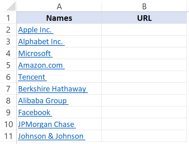
For example, below is a list where I have company names which are hyperlinked to the company website’s URL. When you click on the cell, it will automatically open your default browser (Chrome in my case) and go to that URL.
There are many things you can do with hyperlinks in Excel (such as a link to an external website, link to another sheet/workbook, link to a folder, link to an email, etc.).
In this article, I will cover all you need to know to work with hyperlinks in Excel (including some useful tips and examples).
This Tutorial Covers:
How to Insert Hyperlinks in Excel
There are many different ways to create hyperlinks in Excel:
- Manually type the URL (or copy paste)
- Using the HYPERLINK function
- Using the Insert Hyperlink dialog box
Let’s learn about each of these methods.
Manually Type the URL
When you manually enter a URL in a cell in Excel, or copy and paste it in the cell, Excel automatically converts it into a hyperlink.
Below are the steps that will change a simple URL into a hyperlink:
- Select a cell in which you want to get the hyperlink
- Press F2 to get into the edit mode (or double click on the cell).
- Type the URL and press enter. For example, if I type the URL – https://trumpexcel.com in a cell and hit enter, it will create a hyperlink to it.

Note that you need to add http or https for those URLs where there is no www in it. In case there is www as the prefix, it would create the hyperlink even if you don’t add the http/https.
Similarly, when you copy a URL from the web (or some other document/file) and paste it in a cell in Excel, it will automatically be hyperlinked.
Insert Using the Dialog Box
If you want the text in the cell to be something else other than the URL and want it to link to a specific URL, you can use the insert hyperlink option in Excel.
Below are the steps to enter the hyperlink in a cell using the Insert Hyperlink dialog box:
- Select the cell in which you want the hyperlink
- Enter the text that you want to be hyperlinked. In this case, I am using the text ‘Sumit’s Blog’
- Click the Insert tab.
- Click the links button. This will open the Insert Hyperlink dialog box (You can also use the keyboard shortcut – Control + K).
- In the Insert Hyperlink dialog box, enter the URL in the Address field.
- Press the OK button.


This will insert the hyperlink the cell while the text remains the same.

Insert Using the HYPERLINK Function
Another way to insert a link in Excel can be by using the HYPERLINK Function.
Below is the syntax:
- link_location: This can be the URL of a web-page, a path to a folder or a file in the hard disk, place in a document (such as a specific cell or named range in an Excel worksheet or workbook).
- [friendly_name]: This is an optional argument. This is the text that you want in the cell that has the hyperlink. In case you omit this argument, it will use the link_location text string as the friendly name.
Below is an example where I have the name of companies in one column and their website URL in another column.

Below is the HYPERLINK function to get the result where the text is the company name and it links to the company website.
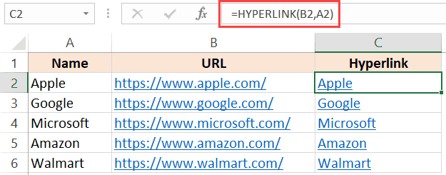
In the examples so far, we have seen how to create hyperlinks to websites.
But you can also create hyperlinks to worksheets in the same workbook, other workbooks, and files and folders on your hard disk.
Let’s see how it can be done.
Create a Hyperlink to a Worksheet in the Same Workbook
Below are the steps to create a hyperlink to Sheet2 in the same workbook:
- Select the cell in which you want the link
- Enter the text that you want to be hyperlinked. In this example, I have used the text ‘Link to Sheet2’.
- Click the Insert tab.
- Click the links button. This will open the Insert Hyperlink dialog box (You can also use the keyboard shortcut – Control + K).
- In the Insert Hyperlink dialog box, select ‘Place in This Document’ option in the left pane.
- Enter the cell which you want to hyperlink (I am going with the default A1).
- Select the sheet that you want to hyperlink (Sheet2 in this case)
- Click OK.

You can also use the same method to link to a defined name (named cell or named range). If you have any named ranges (named cells) in the workbook, these would be listed in under the ‘Defined Names’ category in the ‘Insert Hyperlink’ dialog box.
Apart from the dialog box, there is also a function in Excel that allows you to create hyperlinks.
So instead of using the dialog box, you can instead use the HYPERLINK formula to create a link to a cell in another worksheet.
The below formula will do this:
Below is how this formula works:
- “#” would tell the formula to refer to the same workbook.
- “Sheet2!A1” tells the formula the cell that should be linked to in the same workbook
- “Link to Sheet2” is the text that appears in the cell.
Create a Hyperlink to a File (in the same or different folders)
You can also use the same method to create hyperlinks to other Excel (and non-Excel) files that are in the same folder or are in other folders.
For example, if you want to open a file with the Test.xlsx which is in the same folder as your current file, you can use the below steps:
- Select the cell in which you want the hyperlink
- Click the Insert tab.
- Click the links button. This will open the Insert Hyperlink dialog box (You can also use the keyboard shortcut – Control + K).
- In the Insert Hyperlink dialog box, select ‘Existing File or Webpage’ option in the left pane.
- Select ‘Current folder’ in the Look in options
- Select the file for which you want to create the hyperlink. Note that you can link to any file type (Excel as well as non-Excel files)
- [Optional] Change the Text to Display name if you want to.
- Click OK.

In case you want to link to a file which is not in the same folder, you can Browse the file and then select it. To Browse the file, click on the folder icon in the Insert Hyperlink dialog box (as shown below).

You can also do this using the HYPERLINK function.
The below formula will create a hyperlink that links to a file in the same folder as the current file:
In case the file is not in the same folder, you can copy the address of the file and use it as the link_location.
Create a Hyperlink to a Folder
This one also follows the same methodology.
Below are the steps to create a hyperlink to a folder:
- Copy the folder address for which you want to create the hyperlink
- Select the cell in which you want the hyperlink
- Click the Insert tab.
- Click the links button. This will open the Insert Hyperlink dialog box (You can also use the keyboard shortcut – Control + K).
- In the Insert Hyperlink dialog box, paste folder address
- Click OK.

You can also use the HYPERLINK function to create a hyperlink that points to a folder.
For example, the below formula will create a hyperlink to a folder named TEST on the desktop and as soon as you click on the cell with this formula, it will open this folder.
To use this formula, you will have to change the address of the folder to the one you want to link to.
Create Hyperlink to an Email Address
You can also have hyperlinks which open your default email client (such as Outlook) and have the recipients email and the subject line already filled in the send field.
Below are the steps to create an email hyperlink:
- Select the cell in which you want the hyperlink
- Click the Insert tab.
- Click the links button. This will open the Insert Hyperlink dialog box (You can also use the keyboard shortcut – Control + K).
- In the insert dialog box, click on ‘E-mail Address’ in the ‘Link to’ options
- Enter the E-mail address and the Subject line
- [Optional] Enter the text you want to be displayed in the cell.
- Click OK.

Now when you click on the cell which has the hyperlink, it will open your default email client with the email and subject line pre-filled.
You can also do this using the HYPERLINK function.
The below formula will open the default email client and have one email address already pre-filled.
In case you want to have the subject line as well, you can use the below formula:
In the above formula, I have kept the cc and bcc fields as empty, but you can also these emails if needed.
Remove Hyperlinks
If you only have a few hyperlinks, you can remove these manually, but if you have a lot, you can use a VBA Macro to do this.
Manually Remove Hyperlinks
Below are the steps to remove hyperlinks manually:
- Select the data from which you want to remove hyperlinks.
- Right-click on any of the selected cell.
- Click on the ‘Remove Hyperlink’ option.

The above steps would instantly remove hyperlinks from the selected cells.
In case you want to remove hyperlinks from the entire worksheet, select all the cells and then follow the above steps.
Remove Hyperlinks Using VBA
Below is the VBA code that will remove the hyperlinks from the selected cells:
If you want to remove all the hyperlinks in the worksheet, you can use the below code:
Note that this code will not remove the hyperlinks created using the HYPERLINK function.
You need to add this VBA code in the regular module in the VB Editor.
Here is a detailed guide on how to remove hyperlinks in Excel.
Prevent Excel from Creating Hyperlinks Automatically
For some people, it’s a great feature that Excel automatically converts a URL text to a hyperlink when entered in a cell.
And for some people, it’s an irritation.
If you’re in the latter category, let me show you a way to prevent Excel from automatically creating URLs into hyperlinks.
The reason this happens as there is a setting in Excel that automatically converts ‘Internet and network paths’ into hyperlinks.
Here are the steps to disable this setting in Excel:
- Click the File tab.
- Click on Options.
- In the Excel Options dialog box, click on ‘Proofing’ in the left pane.
- Click on the AutoCorrect Options button.
- In the AutoCorrect dialog box, select the ‘AutoFormat As You Type’ tab.
- Uncheck the option – ‘Internet and network paths with hyperlinks’
- Click OK.
- Close the Excel Options dialog box.


If you’ve completed the following steps, Excel would not automatically turn URLs, email address, and network paths into hyperlinks.
There is no function in Excel that can extract the hyperlink address from a cell.
However, this can be done using the power of VBA.
For example, suppose you have a dataset (as shown below) and you want to extract the hyperlink URL in the adjacent cell.
Let me show you two techniques to extract the hyperlinks from the text in Excel.
Extract Hyperlink in the Adjacent Column
If you want to extract all the hyperlink URLs in one go in an adjacent column, you can so that using the below code:
The above code goes through all the cells in the selection (using the FOR NEXT loop) and extracts the URLs in the adjacent cell.
In case you want to get the hyperlinks in the entire worksheet, you can use the below code:
Note that the above codes wouldn’t work for hyperlinks created using the HYPERLINK function.
The above code works well when you want to get the hyperlinks from a dataset in one go.
But if you have a list of hyperlinks that keeps expanding, you can create a User Defined Function/formula in VBA.
This will allow you to quickly use the cell as the input argument and it will return the hyperlink address in that cell.
Below is the code that will create a UDF for getting the hyperlinks:
Also, in case you select a range of cells (instead of a single cell), this formula will return the hyperlink in the first cell only.
Find Hyperlinks with Specific Text
If you’re working with a huge dataset that has a lot of hyperlinks in it, it could be a challenge when you want to find the ones that have a specific text in it.
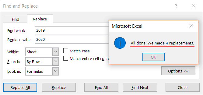
For example, suppose I have a dataset as shown below and I want to find all the cells with hyperlinks that have the text 2019 in it and change it to 2020.

And no.. doing this manually is not an option.
You can do that using a wonderful feature in Excel – Find and Replace.
With this, you can quickly find and select all the cells that have a hyperlink and then change the text 2019 with 2020.
Below are the steps to select all the cells with a hyperlink and the text 2019:
- Select the range in which you want to find the cells with hyperlinks with 2019. In case you want to find in the entire worksheet, select the entire worksheet (click on the small triangle at the top left).
- Click the Home tab.
- In the Editing group, click on Find and Select
- In the drop-down, click on Replace. This will open the Find and Replace dialog box.
- In the Find and Replace dialog box, click on the Options button.This will show more options in the dialog box.
- In the ‘Find What’ options, click on the little downward pointing arrow in the Format button (as shown below).
- Click on the ‘Choose Format From Cell’. This will turn your cursor into a plus icon with a format picker icon.
- Select any cell which has a hyperlink in it. You will notice that the Format gets visible in the box on the left of the Format button. This indicates that the format of the cell you selected has been picked up.
- Enter 2019 in the ‘Find What’ field and 2020 in the ‘Replace with’ field.
- Click on the Replace All button.


In the above data, it will change the text of four cells that have the text 2019 in it and also has a hyperlink.
You can also use this technique to find all the cells with hyperlinks and get a list of it. To do this, instead of clicking on Replace All, click on the Find All button. This will instantly give you a list of all the cell address that has hyperlinks (or hyperlinks with specific text depending on what you’ve searched for).
Selecting a Cell that has a Hyperlink in Excel
While Hyperlinks are useful, there are a few things about it that irritate me.
For example, if you want to select a cell that has a hyperlink in it, Excel would automatically open your default web browser and try to open this URL.
Another irritating thing about it is that sometimes when you have a cell that has a hyperlink in it, it makes the entire cell clickable. So even if you’re clicking on the hyperlinked text directly, it still opens the browser and the URL of the text.
So let me quickly show you how to get rid of these minor irritants.
Select the Cell (without opening the URL)
This is a simple trick.
When you hover the cursor over a cell that has a hyperlink in it, you’ll notice the hand icon (which indicates if you click on it, Excel will open the URL in a browser)
Click the cell anyway and hold the left button of the mouse.
After a second, you’ll notice that the hand cursor icon changes into the plus icon, and now when you leave it, Excel will not open the URL.
Instead, it would select the cell.
Now, you can make any changes in the cell you want.
Neat trick… right?
Select a Cell by clicking on the blank space in the cell
This is another thing that might drive you nuts.
When there is a cell with the hyperlink in it as well as some blank space, and you click on the blank space, it still opens the hyperlink.
Here is a quick fix.
This happens when these cells have the wrap text enabled.
If you disable wrap text for these cells, you will be able to click on the white space on the right of the hyperlink without opening this link.
Some Practical Example of Using Hyperlink
There are useful things you can do when working with hyperlinks in Excel.
In this section, I am going to cover some examples that you may find useful and can use in your day-to-day work.
Example 1 – Create an Index of All Sheets in the Workbook
If you have a workbook with a lot of sheets, you can use a VBA code to quickly create a list of the worksheets and hyperlink these to the sheets.
This could be useful when you have 12-month data in 12 different worksheets and want to create one index sheet that links to all these monthly data worksheets.
Below is the code that will do this:
You can place this code in the regular module in the workbook (in VB Editor)
This code also adds a link to the summary sheet in cell A1 of all the worksheets. In case you don’t want that, you can remove that part from the code.
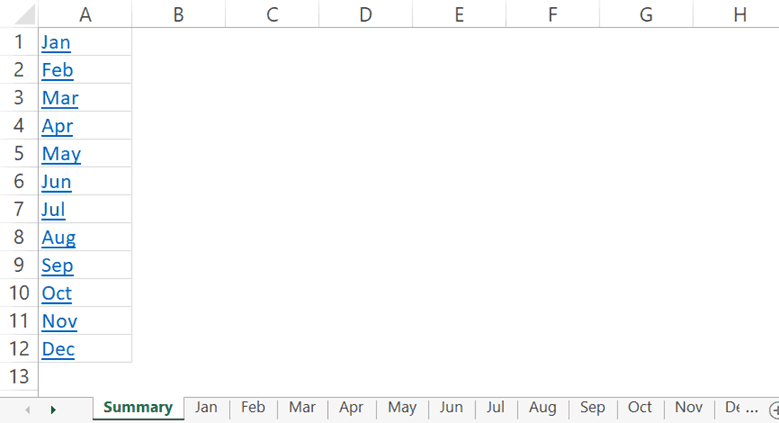
Example 2 – Create Dynamic Hyperlinks
In most cases, when you click on a hyperlink in a cell in Excel, it will take you to a URL or to a cell, file or folder. Normally, these are static URLs which means that a hyperlink will take you to a specific predefined URL/location only.
But you can also use a little bit for Excel formula trickery to create dynamic hyperlinks.
By dynamic hyperlinks, I mean links that are dependent on a user selection and change accordingly.
For example, in the below example, I want the hyperlink in cell E2 to point to the company website based on the drop-down list selected by the user (in cell D2).

This can be done using the below formula in cell E2:
The above formula uses the VLOOKUP function to fetch the URL from the table on the left. The HYPERLINK function then uses this URL to create a hyperlink in the cell with the text – ‘Click here’.
When you change the selection using the drop-down list, the VLOOKUP result will change and would accordingly link to the selected company’s website.
This could be a useful technique when you’re creating a dashboard in Excel. You can make the hyperlinks dynamic depending on the user selection (which could be a drop-down list or a checkbox or a radio button).
Here is a more detailed article of using Dynamic Hyperlinks in Excel.
Example 3 – Quickly Generate Simple Emails Using Hyperlink Function
As I mentioned in this article earlier, you can use the HYPERLINK function to quickly create simple emails (with pre-filled recipient’s emails and the subject line).
Single Recipient Email Id
This would open your default email client with the email id abc@trumpexcel.com in the ‘To’ field.
Multiple Recipients Email Id
For sending the email to multiple recipients, use a comma to separate email ids. This would open the default email client with all the email ids in the ‘To’ field.
Add Recipients in CC and BCC List
To add recipients to CC and BCC list, use question mark ‘?’ when ‘mailto’ argument ends, and join CC and BCC with ‘&’. When you click on the link in excel, it would have the first 2 ids in ‘To’ field, 123@trumpexcel.com in ‘CC’ field and 456@trumpexcel.com in the ‘BCC’ field.
Add Subject Line
You can add a subject line by using the &Subject code. In this case, this would add ‘Excel is Awesome’ in the ‘Subject’ field.
Add Single Line Message in Body
This would add a single line ‘I love Excel’ to the email message body.
Add Multiple Lines Message in Body
To add multiple lines in the body you need to separate each line with %0A. If you wish to introduce two line breaks, add %0A twice, and so on.
Here is a detailed article on how to send emails from Excel.
Hope you found this article useful.
Let me know your thoughts in the comments section.
You May Also Like the Following Excel Tutorials:
Источник
Excel allows having hyperlinks in cells which you can use to directly go to that URL.
For example, below is a list where I have company names which are hyperlinked to the company website’s URL. When you click on the cell, it will automatically open your default browser (Chrome in my case) and go to that URL.
There are many things you can do with hyperlinks in Excel (such as a link to an external website, link to another sheet/workbook, link to a folder, link to an email, etc.).
In this article, I will cover all you need to know to work with hyperlinks in Excel (including some useful tips and examples).
How to Insert Hyperlinks in Excel
There are many different ways to create hyperlinks in Excel:
- Manually type the URL (or copy paste)
- Using the HYPERLINK function
- Using the Insert Hyperlink dialog box
Let’s learn about each of these methods.
Manually Type the URL
When you manually enter a URL in a cell in Excel, or copy and paste it in the cell, Excel automatically converts it into a hyperlink.
Below are the steps that will change a simple URL into a hyperlink:
- Select a cell in which you want to get the hyperlink
- Press F2 to get into the edit mode (or double click on the cell).
- Type the URL and press enter. For example, if I type the URL – https://trumpexcel.com in a cell and hit enter, it will create a hyperlink to it.
Note that you need to add http or https for those URLs where there is no www in it. In case there is www as the prefix, it would create the hyperlink even if you don’t add the http/https.
Similarly, when you copy a URL from the web (or some other document/file) and paste it in a cell in Excel, it will automatically be hyperlinked.
Insert Using the Dialog Box
If you want the text in the cell to be something else other than the URL and want it to link to a specific URL, you can use the insert hyperlink option in Excel.
Below are the steps to enter the hyperlink in a cell using the Insert Hyperlink dialog box:
- Select the cell in which you want the hyperlink
- Enter the text that you want to be hyperlinked. In this case, I am using the text ‘Sumit’s Blog’
- Click the Insert tab.

- Click the links button. This will open the Insert Hyperlink dialog box (You can also use the keyboard shortcut – Control + K).

- In the Insert Hyperlink dialog box, enter the URL in the Address field.
- Press the OK button.
This will insert the hyperlink the cell while the text remains the same.
There are many more things you can do with the ‘Insert Hyperlink’ dialog box (such as create a hyperlink to another worksheet in the same workbook, create a link to a document/folder, create a link to an email address, etc.). These are all covered later in this tutorial.
Insert Using the HYPERLINK Function
Another way to insert a link in Excel can be by using the HYPERLINK Function.
Below is the syntax:
HYPERLINK(link_location, [friendly_name])
- link_location: This can be the URL of a web-page, a path to a folder or a file in the hard disk, place in a document (such as a specific cell or named range in an Excel worksheet or workbook).
- [friendly_name]: This is an optional argument. This is the text that you want in the cell that has the hyperlink. In case you omit this argument, it will use the link_location text string as the friendly name.
Below is an example where I have the name of companies in one column and their website URL in another column.
Below is the HYPERLINK function to get the result where the text is the company name and it links to the company website.
In the examples so far, we have seen how to create hyperlinks to websites.
But you can also create hyperlinks to worksheets in the same workbook, other workbooks, and files and folders on your hard disk.
Let’s see how it can be done.
Create a Hyperlink to a Worksheet in the Same Workbook
Below are the steps to create a hyperlink to Sheet2 in the same workbook:
- Select the cell in which you want the link
- Enter the text that you want to be hyperlinked. In this example, I have used the text ‘Link to Sheet2’.
- Click the Insert tab.
- Click the links button. This will open the Insert Hyperlink dialog box (You can also use the keyboard shortcut – Control + K).
- In the Insert Hyperlink dialog box, select ‘Place in This Document’ option in the left pane.

- Enter the cell which you want to hyperlink (I am going with the default A1).
- Select the sheet that you want to hyperlink (Sheet2 in this case)
- Click OK.
Note: You can also use the same method to create a hyperlink to any cell in the same workbook. For example, if you want to link to a far off cell (say K100), you can do that by using this cell reference in step 6 and selecting the existing sheet in step 7.
You can also use the same method to link to a defined name (named cell or named range). If you have any named ranges (named cells) in the workbook, these would be listed in under the ‘Defined Names’ category in the ‘Insert Hyperlink’ dialog box.
Apart from the dialog box, there is also a function in Excel that allows you to create hyperlinks.
So instead of using the dialog box, you can instead use the HYPERLINK formula to create a link to a cell in another worksheet.
The below formula will do this:
=HYPERLINK("#"&"Sheet2!A1","Link to Sheet2")
Below is how this formula works:
- “#” would tell the formula to refer to the same workbook.
- “Sheet2!A1” tells the formula the cell that should be linked to in the same workbook
- “Link to Sheet2” is the text that appears in the cell.
Create a Hyperlink to a File (in the same or different folders)
You can also use the same method to create hyperlinks to other Excel (and non-Excel) files that are in the same folder or are in other folders.
For example, if you want to open a file with the Test.xlsx which is in the same folder as your current file, you can use the below steps:
- Select the cell in which you want the hyperlink
- Click the Insert tab.
- Click the links button. This will open the Insert Hyperlink dialog box (You can also use the keyboard shortcut – Control + K).
- In the Insert Hyperlink dialog box, select ‘Existing File or Webpage’ option in the left pane.
- Select ‘Current folder’ in the Look in options
- Select the file for which you want to create the hyperlink. Note that you can link to any file type (Excel as well as non-Excel files)

- [Optional] Change the Text to Display name if you want to.
- Click OK.
In case you want to link to a file which is not in the same folder, you can Browse the file and then select it. To Browse the file, click on the folder icon in the Insert Hyperlink dialog box (as shown below).
You can also do this using the HYPERLINK function.
The below formula will create a hyperlink that links to a file in the same folder as the current file:
=HYPERLINK("Test.xlsx","Test File")
In case the file is not in the same folder, you can copy the address of the file and use it as the link_location.
Create a Hyperlink to a Folder
This one also follows the same methodology.
Below are the steps to create a hyperlink to a folder:
- Copy the folder address for which you want to create the hyperlink
- Select the cell in which you want the hyperlink
- Click the Insert tab.
- Click the links button. This will open the Insert Hyperlink dialog box (You can also use the keyboard shortcut – Control + K).
- In the Insert Hyperlink dialog box, paste folder address
- Click OK.
You can also use the HYPERLINK function to create a hyperlink that points to a folder.
For example, the below formula will create a hyperlink to a folder named TEST on the desktop and as soon as you click on the cell with this formula, it will open this folder.
=HYPERLINK("C:UserssumitDesktopTest","Test Folder")
To use this formula, you will have to change the address of the folder to the one you want to link to.
Create Hyperlink to an Email Address
You can also have hyperlinks which open your default email client (such as Outlook) and have the recipients email and the subject line already filled in the send field.
Below are the steps to create an email hyperlink:
- Select the cell in which you want the hyperlink
- Click the Insert tab.
- Click the links button. This will open the Insert Hyperlink dialog box (You can also use the keyboard shortcut – Control + K).
- In the insert dialog box, click on ‘E-mail Address’ in the ‘Link to’ options
- Enter the E-mail address and the Subject line

- [Optional] Enter the text you want to be displayed in the cell.
- Click OK.
Now when you click on the cell which has the hyperlink, it will open your default email client with the email and subject line pre-filled.
You can also do this using the HYPERLINK function.
The below formula will open the default email client and have one email address already pre-filled.
=HYPERLINK("mailto:abc@trumpexcel.com","Send Email")
Note that you need to use mailto: before the email address in the formula. This tells the HYPERLINK function to open the default email client and use the email address that follows.
In case you want to have the subject line as well, you can use the below formula:
=HYPERLINK("mailto:abc@trumpexcel.com,?cc=&bcc=&subject=Excel is Awesome","Generate Email")
In the above formula, I have kept the cc and bcc fields as empty, but you can also these emails if needed.
Here is a detailed guide on how to send emails using the HYPERLINK function.
Remove Hyperlinks
If you only have a few hyperlinks, you can remove these manually, but if you have a lot, you can use a VBA Macro to do this.
Manually Remove Hyperlinks
Below are the steps to remove hyperlinks manually:
- Select the data from which you want to remove hyperlinks.
- Right-click on any of the selected cell.
- Click on the ‘Remove Hyperlink’ option.

The above steps would instantly remove hyperlinks from the selected cells.
In case you want to remove hyperlinks from the entire worksheet, select all the cells and then follow the above steps.
Remove Hyperlinks Using VBA
Below is the VBA code that will remove the hyperlinks from the selected cells:
Sub RemoveAllHyperlinks()
'Code by Sumit Bansal @ trumpexcel.com
Selection.Hyperlinks.Delete
End Sub
If you want to remove all the hyperlinks in the worksheet, you can use the below code:
Sub RemoveAllHyperlinks()
'Code by Sumit Bansal @ trumpexcel.com
ActiveSheet.Hyperlinks.Delete
End Sub
Note that this code will not remove the hyperlinks created using the HYPERLINK function.
You need to add this VBA code in the regular module in the VB Editor.
If you need to remove hyperlinks quite often, you can use the above VBA codes, save it in the Personal Macro Workbook, and add it to your Quick Access Toolbar. This will allow you to remove hyperlinks with a single click and it will be available in all the workbooks on your system.
Here is a detailed guide on how to remove hyperlinks in Excel.
Prevent Excel from Creating Hyperlinks Automatically
For some people, it’s a great feature that Excel automatically converts a URL text to a hyperlink when entered in a cell.
And for some people, it’s an irritation.
If you’re in the latter category, let me show you a way to prevent Excel from automatically creating URLs into hyperlinks.
The reason this happens as there is a setting in Excel that automatically converts ‘Internet and network paths’ into hyperlinks.
Here are the steps to disable this setting in Excel:
- Click the File tab.
- Click on Options.

- In the Excel Options dialog box, click on ‘Proofing’ in the left pane.

- Click on the AutoCorrect Options button.
- In the AutoCorrect dialog box, select the ‘AutoFormat As You Type’ tab.

- Uncheck the option – ‘Internet and network paths with hyperlinks’

- Click OK.
- Close the Excel Options dialog box.
If you’ve completed the following steps, Excel would not automatically turn URLs, email address, and network paths into hyperlinks.
Note that this change is applied to the entire Excel application, and would be applied to all the workbooks that you work with.
Extract Hyperlink URLs (using VBA)
There is no function in Excel that can extract the hyperlink address from a cell.
However, this can be done using the power of VBA.
For example, suppose you have a dataset (as shown below) and you want to extract the hyperlink URL in the adjacent cell.
Let me show you two techniques to extract the hyperlinks from the text in Excel.
Extract Hyperlink in the Adjacent Column
If you want to extract all the hyperlink URLs in one go in an adjacent column, you can so that using the below code:
Sub ExtractHyperLinks()
Dim HypLnk As Hyperlink
For Each HypLnk In Selection.Hyperlinks
    HypLnk.Range.Offset(0, 1).Value = HypLnk.Address
Next HypLnk
End Sub
The above code goes through all the cells in the selection (using the FOR NEXT loop) and extracts the URLs in the adjacent cell.
In case you want to get the hyperlinks in the entire worksheet, you can use the below code:
Sub ExtractHyperLinks()
On Error Resume Next
Dim HypLnk As Hyperlink
For Each HypLnk In ActiveSheet.Hyperlinks
    HypLnk.Range.Offset(0, 1).Value = HypLnk.Address
Next HypLnk
End Sub
Note that the above codes wouldn’t work for hyperlinks created using the HYPERLINK function.
Extract Hyperlink Using a Formula (created with VBA)
The above code works well when you want to get the hyperlinks from a dataset in one go.
But if you have a list of hyperlinks that keeps expanding, you can create a User Defined Function/formula in VBA.
This will allow you to quickly use the cell as the input argument and it will return the hyperlink address in that cell.
Below is the code that will create a UDF for getting the hyperlinks:
Function GetHLink(rng As Range) As String
    If rng(1).Hyperlinks.Count <> 1 Then
        GetHLink = ""
    Else
        GetHLink = rng.Hyperlinks(1).Address
    End If
End Function
Note that this wouldn’t work with Hyperlinks created using the HYPERLINK function.
Also, in case you select a range of cells (instead of a single cell), this formula will return the hyperlink in the first cell only.
Find Hyperlinks with Specific Text
If you’re working with a huge dataset that has a lot of hyperlinks in it, it could be a challenge when you want to find the ones that have a specific text in it.
For example, suppose I have a dataset as shown below and I want to find all the cells with hyperlinks that have the text 2019 in it and change it to 2020.
And no.. doing this manually is not an option.
You can do that using a wonderful feature in Excel – Find and Replace.
With this, you can quickly find and select all the cells that have a hyperlink and then change the text 2019 with 2020.
Below are the steps to select all the cells with a hyperlink and the text 2019:
- Select the range in which you want to find the cells with hyperlinks with 2019. In case you want to find in the entire worksheet, select the entire worksheet (click on the small triangle at the top left).
- Click the Home tab.

- In the Editing group, click on Find and Select

- In the drop-down, click on Replace. This will open the Find and Replace dialog box.

- In the Find and Replace dialog box, click on the Options button.This will show more options in the dialog box.

- In the ‘Find What’ options, click on the little downward pointing arrow in the Format button (as shown below).

- Click on the ‘Choose Format From Cell’. This will turn your cursor into a plus icon with a format picker icon.

- Select any cell which has a hyperlink in it. You will notice that the Format gets visible in the box on the left of the Format button. This indicates that the format of the cell you selected has been picked up.
- Enter 2019 in the ‘Find What’ field and 2020 in the ‘Replace with’ field.
- Click on the Replace All button.


In the above data, it will change the text of four cells that have the text 2019 in it and also has a hyperlink.
You can also use this technique to find all the cells with hyperlinks and get a list of it. To do this, instead of clicking on Replace All, click on the Find All button. This will instantly give you a list of all the cell address that has hyperlinks (or hyperlinks with specific text depending on what you’ve searched for).
Note: This technique works as Excel is able to identify the formatting of the cell that you select and use that as a criterion to find cells. So if you’re finding hyperlinks, make sure you select a cell that has the same kind of formatting. If you select a cell that has a background color or any text formatting, it may not find all the correct cells.
Selecting a Cell that has a Hyperlink in Excel
While Hyperlinks are useful, there are a few things about it that irritate me.
For example, if you want to select a cell that has a hyperlink in it, Excel would automatically open your default web browser and try to open this URL.
Another irritating thing about it is that sometimes when you have a cell that has a hyperlink in it, it makes the entire cell clickable. So even if you’re clicking on the hyperlinked text directly, it still opens the browser and the URL of the text.
So let me quickly show you how to get rid of these minor irritants.
Select the Cell (without opening the URL)
This is a simple trick.
When you hover the cursor over a cell that has a hyperlink in it, you’ll notice the hand icon (which indicates if you click on it, Excel will open the URL in a browser)
![]()
Click the cell anyway and hold the left button of the mouse.
After a second, you’ll notice that the hand cursor icon changes into the plus icon, and now when you leave it, Excel will not open the URL.
![]()
Instead, it would select the cell.
Now, you can make any changes in the cell you want.
Neat trick… right?
Select a Cell by clicking on the blank space in the cell
This is another thing that might drive you nuts.
When there is a cell with the hyperlink in it as well as some blank space, and you click on the blank space, it still opens the hyperlink.
![]()
Here is a quick fix.
This happens when these cells have the wrap text enabled.
If you disable wrap text for these cells, you will be able to click on the white space on the right of the hyperlink without opening this link.
Some Practical Example of Using Hyperlink
There are useful things you can do when working with hyperlinks in Excel.
In this section, I am going to cover some examples that you may find useful and can use in your day-to-day work.
Example 1 – Create an Index of All Sheets in the Workbook
If you have a workbook with a lot of sheets, you can use a VBA code to quickly create a list of the worksheets and hyperlink these to the sheets.
This could be useful when you have 12-month data in 12 different worksheets and want to create one index sheet that links to all these monthly data worksheets.
Below is the code that will do this:
Sub CreateSummary()
'Created by Sumit Bansal of trumpexcel.com
'This code can be used to create summary worksheet with hyperlinks
Dim x As Worksheet
Dim Counter As Integer
Counter = 0
For Each x In Worksheets
Counter = Counter + 1
If Counter = 1 Then GoTo Donothing
    With ActiveCell
        .Value = x.Name
        .Hyperlinks.Add ActiveCell, "", x.Name & "!A1", TextToDisplay:=x.Name, ScreenTip:="Click here to go to the Worksheet"
        With Worksheets(Counter)
            .Range("A1").Value = "Back to " & ActiveSheet.Name
            .Hyperlinks.Add Sheets(x.Name).Range("A1"), "", _
            "'" & ActiveSheet.Name & "'" & "!" & ActiveCell.Address, _
            ScreenTip:="Return to " & ActiveSheet.Name
        End With
    End With
ActiveCell.Offset(1, 0).Select
Donothing:
Next x
End Sub
You can place this code in the regular module in the workbook (in VB Editor)
This code also adds a link to the summary sheet in cell A1 of all the worksheets. In case you don’t want that, you can remove that part from the code.
You can read more about this example here.
Note: This code works when you have the sheet (in which you want the summary of all the worksheets with links) at the beginning. In case it’s not at the beginning, this may not give the right results).
Example 2 – Create Dynamic Hyperlinks
In most cases, when you click on a hyperlink in a cell in Excel, it will take you to a URL or to a cell, file or folder. Normally, these are static URLs which means that a hyperlink will take you to a specific predefined URL/location only.
But you can also use a little bit for Excel formula trickery to create dynamic hyperlinks.
By dynamic hyperlinks, I mean links that are dependent on a user selection and change accordingly.
For example, in the below example, I want the hyperlink in cell E2 to point to the company website based on the drop-down list selected by the user (in cell D2).
This can be done using the below formula in cell E2:
=HYPERLINK(VLOOKUP(D2,$A$2:$B$6,2,0), "Click here")
The above formula uses the VLOOKUP function to fetch the URL from the table on the left. The HYPERLINK function then uses this URL to create a hyperlink in the cell with the text – ‘Click here’.
When you change the selection using the drop-down list, the VLOOKUP result will change and would accordingly link to the selected company’s website.
This could be a useful technique when you’re creating a dashboard in Excel. You can make the hyperlinks dynamic depending on the user selection (which could be a drop-down list or a checkbox or a radio button).
Here is a more detailed article of using Dynamic Hyperlinks in Excel.
Example 3 – Quickly Generate Simple Emails Using Hyperlink Function
As I mentioned in this article earlier, you can use the HYPERLINK function to quickly create simple emails (with pre-filled recipient’s emails and the subject line).
Single Recipient Email Id
=HYPERLINK("mailto:abc@trumpexcel.com","Generate Email")
This would open your default email client with the email id abc@trumpexcel.com in the ‘To’ field.
Multiple Recipients Email Id
=HYPERLINK("mailto:abc@trumpexcel.com,def@trumpexcel.com","Generate Email")
For sending the email to multiple recipients, use a comma to separate email ids. This would open the default email client with all the email ids in the ‘To’ field.
Add Recipients in CC and BCC List
=HYPERLINK("mailto:abc@trumpexcel.com,def@trumpexcel.com?cc=123@trumpexcel.com&bcc=456@trumpexcel.com","Generate Email")
To add recipients to CC and BCC list, use question mark ‘?’ when ‘mailto’ argument ends, and join CC and BCC with ‘&’. When you click on the link in excel, it would have the first 2 ids in ‘To’ field, 123@trumpexcel.com in ‘CC’ field and 456@trumpexcel.com in the ‘BCC’ field.
Add Subject Line
=HYPERLINK("mailto:abc@trumpexcel.com,def@trumpexcel.com?cc=123@trumpexcel.com&bcc=456@trumpexcel.com&subject=Excel is Awesome","Generate Email")
You can add a subject line by using the &Subject code. In this case, this would add ‘Excel is Awesome’ in the ‘Subject’ field.
Add Single Line Message in Body
=HYPERLINK("mailto:abc@trumpexcel.com,def@trumpexcel.com?cc=123@trumpexcel.com&bcc=456@trumpexcel.com&subject=Excel is Awesome&body=I love Excel","Email Trump Excel")
This would add a single line ‘I love Excel’ to the email message body.
Add Multiple Lines Message in Body
=HYPERLINK("mailto:abc@trumpexcel.com,def@trumpexcel.com?cc=123@trumpexcel.com&bcc=456@trumpexcel.com&subject=Excel is Awesome&body=I love Excel.%0AExcel is Awesome","Generate Email")
To add multiple lines in the body you need to separate each line with %0A. If you wish to introduce two line breaks, add %0A twice, and so on.
Here is a detailed article on how to send emails from Excel.
Hope you found this article useful.
Let me know your thoughts in the comments section.
You May Also Like the Following Excel Tutorials:
- Excel AutoCorrect
- How to Find External Links and References in Excel
- 100+ Excel Interview Questions & Answers
- Excel Text to Columns
- Excel Sparklines