
For quick access to related information in another file or on a web page, you can insert a hyperlink in a worksheet cell. You can also insert links in specific chart elements.
Note: Most of the screen shots in this article were taken in Excel 2016. If you have a different version your view might be slightly different, but unless otherwise noted, the functionality is the same.
-
On a worksheet, click the cell where you want to create a link.
You can also select an object, such as a picture or an element in a chart, that you want to use to represent the link.
-
On the Insert tab, in the Links group, click Link
 .
.
You can also right-click the cell or graphic and then click Link on the shortcut menu, or you can press Ctrl+K.
-
-
Under Link to, click Create New Document.
-
In the Name of new document box, type a name for the new file.
Tip: To specify a location other than the one shown under Full path, you can type the new location preceding the name in the Name of new document box, or you can click Change to select the location that you want and then click OK.
-
Under When to edit, click Edit the new document later or Edit the new document now to specify when you want to open the new file for editing.
-
In the Text to display box, type the text that you want to use to represent the link.
-
To display helpful information when you rest the pointer on the link, click ScreenTip, type the text that you want in the ScreenTip text box, and then click OK.
 .
.-
On a worksheet, click the cell where you want to create a link.
You can also select an object, such as a picture or an element in a chart, that you want to use to represent the link.
-
On the Insert tab, in the Links group, click Link
.
You can also right-click the cell or object and then click Link on the shortcut menu, or you can press Ctrl+K.
-
-
Under Link to, click Existing File or Web Page.
-
Do one of the following:
-
To select a file, click Current Folder, and then click the file that you want to link to.
You can change the current folder by selecting a different folder in the Look in list.
-
To select a web page, click Browsed Pages and then click the web page that you want to link to.
-
To select a file that you recently used, click Recent Files, and then click the file that you want to link to.
-
To enter the name and location of a known file or web page that you want to link to, type that information in the Address box.
-
To locate a web page, click Browse the Web
, open the web page that you want to link to, and then switch back to Excel without closing your browser.
-
-
If you want to create a link to a specific location in the file or on the web page, click Bookmark, and then double-click the bookmark that you want.
Note: The file or web page that you are linking to must have a bookmark.
-
In the Text to display box, type the text that you want to use to represent the link.
-
To display helpful information when you rest the pointer on the link, click ScreenTip, type the text that you want in the ScreenTip text box, and then click OK.
 , open the web page that you want to link to, and then switch back to Excel without closing your browser.
To link to a location in the current workbook or another workbook, you can either define a name for the destination cells or use a cell reference.
-
To use a name, you must name the destination cells in the destination workbook.
How to name a cell or a range of cells
-
Select the cell, range of cells, or nonadjacent selections that you want to name.
-
Click the Name box at the left end of the formula bar
.
Name box -
In the Name box, type the name for the cells, and then press Enter.
Note: Names can’t contain spaces and must begin with a letter.
-
-
On a worksheet of the source workbook, click the cell where you want to create a link.
You can also select an object, such as a picture or an element in a chart, that you want to use to represent the link.
-
On the Insert tab, in the Links group, click Link
.
You can also right-click the cell or object and then click Link on the shortcut menu, or you can press Ctrl+K.
-
-
Under Link to, do one of the following:
-
To link to a location in your current workbook, click Place in This Document.
-
To link to a location in another workbook, click Existing File or Web Page, locate and select the workbook that you want to link to, and then click Bookmark.
-
-
Do one of the following:
-
In the Or select a place in this document box, under Cell Reference, click the worksheet that you want to link to, type the cell reference in the Type in the cell reference box, and then click OK.
-
In the list under Defined Names, click the name that represents the cells that you want to link to, and then click OK.
-
-
In the Text to display box, type the text that you want to use to represent the link.
-
To display helpful information when you rest the pointer on the link, click ScreenTip, type the text that you want in the ScreenTip text box, and then click OK.
 .
.
 Name box
You can use the HYPERLINK function to create a link that opens a document that is stored on a network server, an intranet, or the Internet. When you click the cell that contains the HYPERLINK function, Excel opens the file that is stored at the location of the link.
Syntax
HYPERLINK(link_location,friendly_name)
Link_location is the path and file name to the document to be opened as text. Link_location can refer to a place in a document — such as a specific cell or named range in an Excel worksheet or workbook, or to a bookmark in a Microsoft Word document. The path can be to a file stored on a hard disk drive, or the path can be a universal naming convention (UNC) path on a server (in Microsoft Excel for Windows) or a Uniform Resource Locator (URL) path on the Internet or an intranet.
-
Link_location can be a text string enclosed in quotation marks or a cell that contains the link as a text string.
-
If the jump specified in link_location does not exist or can’t be navigated, an error appears when you click the cell.
Friendly_name is the jump text or numeric value that is displayed in the cell. Friendly_name is displayed in blue and is underlined. If friendly_name is omitted, the cell displays the link_location as the jump text.
-
Friendly_name can be a value, a text string, a name, or a cell that contains the jump text or value.
-
If friendly_name returns an error value (for example, #VALUE!), the cell displays the error instead of the jump text.
Examples
The following example opens a worksheet named Budget Report.xls that is stored on the Internet at the location named example.microsoft.com/report and displays the text «Click for report»:
=HYPERLINK(«http://example.microsoft.com/report/budget report.xls», «Click for report»)
The following example creates a link to cell F10 on the worksheet named Annual in the workbook Budget Report.xls, which is stored on the Internet at the location named example.microsoft.com/report. The cell on the worksheet that contains the link displays the contents of cell D1 as the jump text:
=HYPERLINK(«[http://example.microsoft.com/report/budget report.xls]Annual!F10», D1)
The following example creates a link to the range named DeptTotal on the worksheet named First Quarter in the workbook Budget Report.xls, which is stored on the Internet at the location named example.microsoft.com/report. The cell on the worksheet that contains the link displays the text «Click to see First Quarter Department Total»:
=HYPERLINK(«[http://example.microsoft.com/report/budget report.xls]First Quarter!DeptTotal», «Click to see First Quarter Department Total»)
To create a link to a specific location in a Microsoft Word document, you must use a bookmark to define the location you want to jump to in the document. The following example creates a link to the bookmark named QrtlyProfits in the document named Annual Report.doc located at example.microsoft.com:
=HYPERLINK(«[http://example.microsoft.com/Annual Report.doc]QrtlyProfits», «Quarterly Profit Report»)
In Excel for Windows, the following example displays the contents of cell D5 as the jump text in the cell and opens the file named 1stqtr.xls, which is stored on the server named FINANCE in the Statements share. This example uses a UNC path:
=HYPERLINK(«\FINANCEStatements1stqtr.xls», D5)
The following example opens the file 1stqtr.xls in Excel for Windows that is stored in a directory named Finance on drive D, and displays the numeric value stored in cell H10:
=HYPERLINK(«D:FINANCE1stqtr.xls», H10)
In Excel for Windows, the following example creates a link to the area named Totals in another (external) workbook, Mybook.xls:
=HYPERLINK(«[C:My DocumentsMybook.xls]Totals»)
In Microsoft Excel for the Macintosh, the following example displays «Click here» in the cell and opens the file named First Quarter that is stored in a folder named Budget Reports on the hard drive named Macintosh HD:
=HYPERLINK(«Macintosh HD:Budget Reports:First Quarter», «Click here»)
You can create links within a worksheet to jump from one cell to another cell. For example, if the active worksheet is the sheet named June in the workbook named Budget, the following formula creates a link to cell E56. The link text itself is the value in cell E56.
=HYPERLINK(«[Budget]June!E56», E56)
To jump to a different sheet in the same workbook, change the name of the sheet in the link. In the previous example, to create a link to cell E56 on the September sheet, change the word «June» to «September.»
When you click a link to an email address, your email program automatically starts and creates an email message with the correct address in the To box, provided that you have an email program installed.
-
On a worksheet, click the cell where you want to create a link.
You can also select an object, such as a picture or an element in a chart, that you want to use to represent the link.
-
On the Insert tab, in the Links group, click Link
.
You can also right-click the cell or object and then click Link on the shortcut menu, or you can press Ctrl+K.
-
-
Under Link to, click E-mail Address.
-
In the E-mail address box, type the email address that you want.
-
In the Subject box, type the subject of the email message.
Note: Some web browsers and email programs may not recognize the subject line.
-
In the Text to display box, type the text that you want to use to represent the link.
-
To display helpful information when you rest the pointer on the link, click ScreenTip, type the text that you want in the ScreenTip text box, and then click OK.
You can also create a link to an email address in a cell by typing the address directly in the cell. For example, a link is created automatically when you type an email address, such as someone@example.com.
You can insert one or more external reference (also called links) from a workbook to another workbook that is located on your intranet or on the Internet. The workbook must not be saved as an HTML file.
-
Open the source workbook and select the cell or cell range that you want to copy.
-
On the Home tab, in the Clipboard group, click Copy.
-
Switch to the worksheet that you want to place the information in, and then click the cell where you want the information to appear.
-
On the Home tab, in the Clipboard group, click Paste Special.
-
Click Paste Link.
Excel creates an external reference link for the cell or each cell in the cell range.

Note: You may find it more convenient to create an external reference link without opening the workbook on the web. For each cell in the destination workbook where you want the external reference link, click the cell, and then type an equal sign (=), the URL address, and the location in the workbook. For example:
=’http://www.someones.homepage/[file.xls]Sheet1′!A1
=’ftp.server.somewhere/file.xls’!MyNamedCell
To select a hyperlink without activating the link to its destination, do one of the following:
-
Click the cell that contains the link, hold the mouse button until the pointer becomes a cross
, and then release the mouse button. -
Use the arrow keys to select the cell that contains the link.
-
If the link is represented by a graphic, hold down Ctrl, and then click the graphic.
 , and then release the mouse button.
You can change an existing link in your workbook by changing its destination, its appearance, or the text or graphic that is used to represent it.
Change the destination of a link
-
Select the cell or graphic that contains the link that you want to change.
Tip: To select a cell that contains a link without going to the link destination, click the cell and hold the mouse button until the pointer becomes a cross
, and then release the mouse button. You can also use the arrow keys to select the cell. To select a graphic, hold down Ctrl and click the graphic.-
On the Insert tab, in the Links group, click Link.
You can also right-click the cell or graphic and then click Edit Link on the shortcut menu, or you can press Ctrl+K.
-
-
In the Edit Hyperlink dialog box, make the changes that you want.
Note: If the link was created by using the HYPERLINK worksheet function, you must edit the formula to change the destination. Select the cell that contains the link, and then click the formula bar to edit the formula.
You can change the appearance of all link text in the current workbook by changing the cell style for links.
-
On the Home tab, in the Styles group, click Cell Styles.
-
Under Data and Model, do the following:
-
To change the appearance of links that have not been clicked to go to their destinations, right-click Link, and then click Modify.
-
To change the appearance of links that have been clicked to go to their destinations, right-click Followed Link, and then click Modify.
Note: The Link cell style is available only when the workbook contains a link. The Followed Link cell style is available only when the workbook contains a link that has been clicked.
-
-
In the Style dialog box, click Format.
-
On the Font tab and Fill tab, select the formatting options that you want, and then click OK.
Notes:
-
The options that you select in the Format Cells dialog box appear as selected under Style includes in the Style dialog box. You can clear the check boxes for any options that you don’t want to apply.
-
Changes that you make to the Link and Followed Link cell styles apply to all links in the current workbook. You can’t change the appearance of individual links.
-
-
Select the cell or graphic that contains the link that you want to change.
Tip: To select a cell that contains a link without going to the link destination, click the cell and hold the mouse button until the pointer becomes a cross
, and then release the mouse button. You can also use the arrow keys to select the cell. To select a graphic, hold down Ctrl and click the graphic. -
Do one or more of the following:
-
To change the link text, click in the formula bar, and then edit the text.
-
To change the format of a graphic, right-click it, and then click the option that you need to change its format.
-
To change text in a graphic, double-click the selected graphic, and then make the changes that you want.
-
To change the graphic that represents the link, insert a new graphic, make it a link with the same destination, and then delete the old graphic and link.
-
-
Right-click the hyperlink that you want to copy or move, and then click Copy or Cut on the shortcut menu.
-
Right-click the cell that you want to copy or move the link to, and then click Paste on the shortcut menu.
By default, unspecified paths to hyperlink destination files are relative to the location of the active workbook. Use this procedure when you want to set a different default path. Each time that you create a link to a file in that location, you only have to specify the file name, not the path, in the Insert Hyperlink dialog box.
Follow one of the steps depending on the Excel version you are using:
-
In Excel 2016, Excel 2013, and Excel 2010:
-
Click the File tab.
-
Click Info.
-
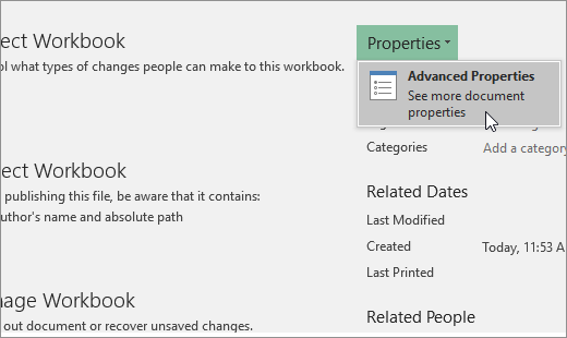
Click Properties, and then select Advanced Properties.
-
In the Summary tab, in the Hyperlink base text box, type the path that you want to use.
Note: You can override the link base address by using the full, or absolute, address for the link in the Insert Hyperlink dialog box.
-
-
In Excel 2007:
-
Click the Microsoft Office Button
, click Prepare, and then click Properties. -
In the Document Information Panel, click Properties, and then click Advanced Properties.
-
Click the Summary tab.
-
In the Hyperlink base box, type the path that you want to use.
Note: You can override the link base address by using the full, or absolute, address for the link in the Insert Hyperlink dialog box.
-
 , click Prepare, and then click Properties.
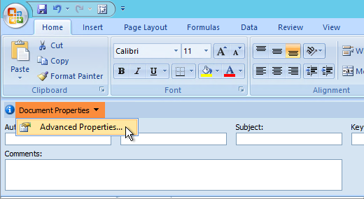
To delete a link, do one of the following:
-
To delete a link and the text that represents it, right-click the cell that contains the link, and then click Clear Contents on the shortcut menu.
-
To delete a link and the graphic that represents it, hold down Ctrl and click the graphic, and then press Delete.
-
To turn off a single link, right-click the link, and then click Remove Link on the shortcut menu.
-
To turn off several links at once, do the following:
-
In a blank cell, type the number 1.
-
Right-click the cell, and then click Copy on the shortcut menu.
-
Hold down Ctrl and select each link that you want to turn off.
Tip: To select a cell that has a link in it without going to the link destination, click the cell and hold the mouse button until the pointer becomes a cross
, and then release the mouse button. -
On the Home tab, in the Clipboard group, click the arrow below Paste, and then click Paste Special.
-
Under Operation, click Multiply, and then click OK.
-
On the Home tab, in the Styles group, click Cell Styles.
-
Under Good, Bad, and Neutral, select Normal.
-
A link opens another page or file when you click it. The destination is frequently another web page, but it can also be a picture, or an email address, or a program. The link itself can be text or a picture.
When a site user clicks the link, the destination is shown in a Web browser, opened, or run, depending on the type of destination. For example, a link to a page shows the page in the web browser, and a link to an AVI file opens the file in a media player.
How links are used
You can use links to do the following:
-
Navigate to a file or web page on a network, intranet, or Internet
-
Navigate to a file or web page that you plan to create in the future
-
Send an email message
-
Start a file transfer, such as downloading or an FTP process
When you point to text or a picture that contains a link, the pointer becomes a hand  , indicating that the text or picture is something that you can click.
What a URL is and how it works
When you create a link, its destination is encoded as a Uniform Resource Locator (URL), such as:
http://example.microsoft.com/news.htm
file://ComputerName/SharedFolder/FileName.htm
A URL contains a protocol, such as HTTP, FTP, or FILE, a Web server or network location, and a path and file name. The following illustration defines the parts of the URL:
1. Protocol used (http, ftp, file)
2. Web server or network location
3. Path
4. File name
Absolute and relative links
An absolute URL contains a full address, including the protocol, the Web server, and the path and file name.
A relative URL has one or more missing parts. The missing information is taken from the page that contains the URL. For example, if the protocol and web server are missing, the web browser uses the protocol and domain, such as .com, .org, or .edu, of the current page.
It is common for pages on the web to use relative URLs that contain only a partial path and file name. If the files are moved to another server, any links will continue to work as long as the relative positions of the pages remain unchanged. For example, a link on Products.htm points to a page named apple.htm in a folder named Food; if both pages are moved to a folder named Food on a different server, the URL in the link will still be correct.
In an Excel workbook, unspecified paths to link destination files are by default relative to the location of the active workbook. You can set a different base address to use by default so that each time that you create a link to a file in that location, you only have to specify the file name, not the path, in the Insert Hyperlink dialog box.
-
On a worksheet, select the cell where you want to create a link.
-
On the Insert tab, select Hyperlink.
You can also right-click the cell and then select Hyperlink… on the shortcut menu, or you can press Ctrl+K.
-
Under Display Text:, type the text that you want to use to represent the link.
-
Under URL:, type the complete Uniform Resource Locator (URL) of the webpage you want to link to.
-
Select OK.
To link to a location in the current workbook, you can either define a name for the destination cells or use a cell reference.
-
To use a name, you must name the destination cells in the workbook.
How to define a name for a cell or a range of cells
Note: In Excel for the Web, you can’t create named ranges. You can only select an existing named range from the Named Ranges control. Alternately, you can open the file in the Excel desktop app, create a named range there, and then access this option from Excel for the web.
-
Select the cell or range of cells that you want to name.
-
On the Name Box box at the left end of the formula bar
, type the name for the cells, and then press Enter.Note: Names can’t contain spaces and must begin with a letter.
-
-
On the worksheet, select the cell where you want to create a link.
-
On the Insert tab, select Hyperlink.
You can also right-click the cell and then select Hyperlink… on the shortcut menu, or you can press Ctrl+K.
-
Under Display Text:, type the text that you want to use to represent the link.
-
Under Place in this document:, enter the defined name or cell reference.
-
Select OK.
When you click a link to an email address, your email program automatically starts and creates an email message with the correct address in the To box, provided that you have an email program installed.
-
On a worksheet, select the cell where you want to create a link.
-
On the Insert tab, select Hyperlink.
You can also right-click the cell and then select Hyperlink… on the shortcut menu, or you can press Ctrl+K.
-
Under Display Text:, type the text that you want to use to represent the link.
-
Under E-mail address:, type the email address that you want.
-
Select OK.
You can also create a link to an email address in a cell by typing the address directly in the cell. For example, a link is created automatically when you type an email address, such as someone@example.com.
You can use the HYPERLINK function to create a link to a URL.
Note: The Link_location can be a text string enclosed in quotation marks or a reference to a cell that contains the link as a text string.
To select a hyperlink without activating the link to its destination, do any of the following:
-
Select a cell by clicking it when the pointer is an arrow.
-
Use the arrow keys to select the cell that contains the link.
You can change an existing link in your workbook by changing its destination, its appearance, or the text that is used to represent it.
-
Select the cell that contains the link that you want to change.
Tip: To select a hyperlink without activating the link to its destination, use the arrow keys to select the cell that contains the link.
-
On the Insert tab, select Hyperlink.
You can also right-click the cell or graphic and then select Edit Hyperlink… on the shortcut menu, or you can press Ctrl+K.
-
In the Edit Hyperlink dialog box, make the changes that you want.
Note: If the link was created by using the HYPERLINK worksheet function, you must edit the formula to change the destination. Select the cell that contains the link, and then select the formula bar to edit the formula.
-
Right-click the hyperlink that you want to copy or move, and then select Copy or Cut on the shortcut menu.
-
Right-click the cell that you want to copy or move the link to, and then select Paste on the shortcut menu.
To delete a link, do one of the following:
-
To delete a link, select the cell and press Delete.
-
To turn off a link (delete the link but keep the text that represents it), right-click the cell and then select Remove Hyperlink.
Need more help?
You can always ask an expert in the Excel Tech Community or get support in the Answers community.
See Also
Remove or turn off links
![]()
Download Article
Step-by-step guide to creating hyperlinks in Excel
![]()
Download Article
- Linking to a New File
- Linking to an Existing File or Webpage
- Linking Within the Document
- Creating an Email Address Hyperlink
- Using the HYPERLINK Function
- Creating a Link to a Workbook on the Web
- Video
- Q&A
- Tips
- Warnings
|
|
|
|
|
|
|
|
|
This wikiHow teaches you how to create a link to a file, folder, webpage, new document, email, or external reference in Microsoft Excel. You can do this on both the Windows and Mac versions of Excel. Creating a hyperlink is easy using Excel’s built-in link tool. Alternatively, you can use the HYPERLINK function to quickly link to a location.
Things You Should Know
- You can link to a new file, existing file, webpage, email, or location in your document.
- Use the HYPERLINK function if you already have the link location.
- Create an external reference link to another workbook to insert a cell value into your workbook.
-
1
Open an Excel document. Double-click the Excel document in which you want to insert a hyperlink.
- You can also open a new document by double-clicking the Excel icon and clicking Blank Workbook.
-
2
Select a cell. This should be a cell into which you want to insert your hyperlink.
Advertisement
-
3
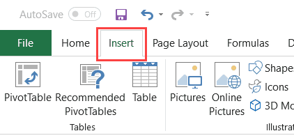
Click Insert. This tab is in the green ribbon at the top of the Excel window. Clicking Insert opens a toolbar directly below the green ribbon.[1]
- If you’re on a Mac, note that there’s an Excel Insert tab and an Insert menu item in your Mac’s menu bar. Select the Excel Insert tab.
-
4
Click Link. It’s toward the right side of the Insert toolbar in the «Links» section. Doing so opens a pop up menu.
-
5
Click Insert Link. It’s at the bottom of the Link pop up menu. This opens the Insert Hyperlink window.
-
6
Click Create New Document. This tab is on the left side of the pop-up window, under “Link to:”.
- This option is not available on some versions of Excel. You’ll need to create the new document before making the hyperlink, then use the Existing File or Web Page option.
-
7
Enter the hyperlink’s text. Type the text that you want to see displayed into the «Text to display» field. This is the box above the “Name of new document” field.
-
8
Type in a name for the new document. Do so in the «Name of new document» field.
-
9
Click OK. It’s at the bottom of the window. By default, this will create and open a new spreadsheet document, then create a link to it in the cell that you selected in the other spreadsheet document.
- You can also select the «Edit the new document later» option before clicking OK to create the spreadsheet and the link without opening the spreadsheet.
- If something goes wrong with the hyperlink, see our guide for fixing a hyperlink in Excel.


Advertisement
-
1
Open an Excel document. Double-click the Excel document in which you want to insert a hyperlink.
- You can also open a new document by double-clicking the Excel icon and then clicking Blank Workbook.
- Hyperlinks are a great way to organize and connect information across multiple Excel documents. You can also easily create hyperlinks in PowerPoint if you have a presentation coming up.
-
2
Select a cell. This should be a cell into which you want to insert your hyperlink.
-
3
Click Insert. This tab is in the green ribbon at the top of the Excel window. Clicking Insert opens a toolbar directly below the green ribbon.
- If you’re on a Mac, note that there’s an Excel Insert tab and an Insert menu item in your Mac’s menu bar. Select the Excel Insert tab.
-
4
Click Link. It’s toward the right side of the Insert toolbar in the «Links» section. Doing so opens a pop up menu.
-
5
Click Insert Link. It’s at the bottom of the Link pop up menu. This opens the Insert Hyperlink window.
-
6
Click the Existing File or Web Page. It’s on the left side of the window.
-
7
Enter the hyperlink’s text. Type the text that you want to see displayed into the «Text to display» field.
- If you don’t do this, your hyperlink’s text will just be the folder path to the linked item.
-
8
Select a destination. You can choose a file location on your computer, enter an address of a file or web page, or browse the internet. Here are the destination options:
- Current Folder — Search for files in your Documents or Desktop folder.
- Browsed Pages — Search through recently viewed web pages.
- Recent Files — Search through recently opened Excel files.
- Type in the location and name of a web page or file into the “Address” field. For example, this could be a URL to a website.
- Click the Browse the Web button (a globe behind a magnifying glass). Go to the web page you’re linking to, then go back to Excel. Don’t close your browser!
-
9
Select a file or webpage. Click the file, folder, or web address to which you want to link. A path to the folder will appear in the «Address» text box at the bottom of the window.
-
10
Click OK. It’s at the bottom of the page. Doing so creates your hyperlink in your specified cell.
- Note that if you move the item to which you linked, the hyperlink will no longer work.


Advertisement
-
1
Open an Excel document. Double-click the Excel document in which you want to insert a hyperlink. This method links to a cell or sheet in your workbook. For example, if you’re tracking your bills in Excel, you can link to a summary sheet from your data sheet.
- You can also open a new document by double-clicking the Excel icon and then clicking Blank Workbook.
-
2
Select a cell. This should be a cell into which you want to insert your hyperlink.
-
3
Click Insert. This tab is in the green ribbon at the top of the Excel window. Clicking Insert opens a toolbar directly below the green ribbon.
- If you’re on a Mac, note that there’s an Excel Insert tab and an Insert menu item in your Mac’s menu bar. Select the Excel Insert tab.
-
4
Click Link. It’s toward the right side of the Insert toolbar in the «Links» section. Doing so opens a pop up menu.
-
5
Click Insert Link. It’s at the bottom of the Link pop up menu. This opens the Insert Hyperlink window.
-
6
Click the Place in This Document. It’s on the left side of the window.
-
7
Select a location in the Excel document. You have two options for selecting a location:
- Under “Type the cell reference,” type in the cell you want to link to.
- Alternatively, under “Or select a place in this document,” click a sheet name or defined name.
-
8
Enter the hyperlink’s text. Type the text that you want to see displayed into the «Text to display» field.
- If you don’t do this, your hyperlink’s text will just be the linked cell’s name.
-
9
Click OK. This will create your link in the selected cell. If you click the hyperlink, Excel will automatically highlight the linked cell or take you to the sheet you selected.
- For general Excel tips, see our intro guide to Excel.


Advertisement
-
1
Open an Excel document. Double-click the Excel document in which you want to insert a hyperlink.
- You can also open a new document by double-clicking the Excel icon and then clicking Blank Workbook.
-
2
Select a cell. This should be a cell into which you want to insert your hyperlink.
-
3
Click Insert. This tab is in the green ribbon at the top of the Excel window. Clicking Insert opens a toolbar directly below the green ribbon.
- If you’re on a Mac, note that there’s an Excel Insert tab and an Insert menu item in your Mac’s menu bar. Select the Excel Insert tab.
-
4
Click Link. It’s toward the right side of the Insert toolbar in the «Links» section. Doing so opens a pop up menu.
-
5
Click Insert Link. It’s at the bottom of the Link pop up menu. This opens the Insert Hyperlink window.
-
6
Click E-mail Address. It’s on the left side of the window.
-
7
Enter the hyperlink’s text. Type the text that you want to see displayed into the «Text to display» field.
- If you don’t change the hyperlink’s text, the email address will display as itself.
-
8
Enter the email address. Type the email address that you want to hyperlink into the «E-mail address» field.
- You can also add a prewritten subject to the «Subject» field, which will cause the hyperlinked email to open a new email message with the subject already filled in.
-
9
Click OK. This button is at the bottom of the window.
- Clicking this email link will automatically open an installed email program with a new email to the specified address.


Advertisement
-
1
Open an Excel document. Double-click the Excel document in which you want to insert a hyperlink.
- You can also open a new document by double-clicking the Excel icon and then clicking Blank Workbook.
-
2
Select a cell. This should be a cell into which you want to insert your hyperlink.
-
3
Type =HYPERLINK(). This function creates a hyperlink to a document on the Internet, an intranet, or a server. This function has two parameters:[2]
- HYPERLINK(link_location,friendly_name)
- link_location is where you type in the path to the file and the file name.
- friendly_name is the text shown for the hyperlink in your Excel spreadsheet. This parameter is optional.
-
4
Add the link location and friendly name. To do so:
- In the parenthesis of the HYPERLINK function, type the file path and file name for the document you want to link to.
- Add a comma (,).
- Type the name you want to appear for the hyperlink.
-
5
Press ↵ Enter. This will confirm the HYPERLINK formula and create the hyperlink in the selected cell. Clicking the link will open the specified file.


Advertisement
-
1
Open an Excel document. Double-click the Excel document in which you want to insert a hyperlink.
- You can also open a new document by double-clicking the Excel icon and then clicking Blank Workbook.
-
2
Open the workbook you want to link to. This can be referred to as the source workbook. This method creates an external reference link to a workbook on the Internet or your intranet.
-
3
Select the cell you want to link to in the source workbook. This will place a green box around the cell.
-
4
Copy the cell. You’ll need to copy the cell to reference it in your workbook. To copy it:
- Go to the Home tab.
- Click Copy in the “Clipboard” section. This button has an icon of two pieces of paper.
-
5
Go to your workbook. This is the workbook that you want to place the external reference link in.
-
6
Select the cell you want to place the link in. You can place the link in any sheet of your workbook.
-
7
Click the Home tab. This will open the Home toolbar.
-
8
Click the Paste drop down button. This is the button below the clipboard with a down arrow. This opens the Paste drop down menu.
-
9
Click the Paste Link button. This is two chains linked together in front of a clipboard in the Paste drop down menu. The value of the external reference will appear in the cell you selected.
- To see the external reference location, select the cell with the external reference. Then, check the Formula Bar for the location.


Advertisement
Add New Question
-
Question
How do I put a hyperlink in a text box?

Right-click on the cell into which you wish to insert the link. Choose ‘Link’ on the menu which pops up, then insert the URL at the bottom of the little Link Setup Window.
-
Question
My Excel chart hyperlinks work on my computer, but not on the computers of folks I send the chart to. Why?
MS Office applications routinely disable links and other potentially harmful content whenever you open a file created on another PC or downloaded from the Internet. A warning message is displayed at the top of the document. The user then has the choice to trust the source of the document, which enables all content, or to view it in «Compatibility Mode,» with potentially harmful content disabled.
-
Question
The hyperlink option in the drop down menu is shaded and I can’t click on it. What should I do?
Highlight the text you want to add a hyperlink to, then click hyperlink.
Ask a Question
200 characters left
Include your email address to get a message when this question is answered.
Submit
Advertisement
Video
Thanks for submitting a tip for review!
Advertisement
-
If you move a file connected to an Excel spreadsheet by hyperlink to a new location, you will have to edit the hyperlink to include the new file location.
Advertisement
About This Article
Thanks to all authors for creating a page that has been read 486,649 times.
Is this article up to date?
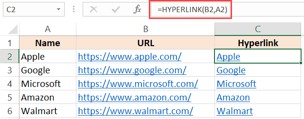
Excel allows having hyperlinks in cells which you can use to directly go to that URL.
For example, below is a list where I have company names which are hyperlinked to the company website’s URL. When you click on the cell, it will automatically open your default browser (Chrome in my case) and go to that URL.
There are many things you can do with hyperlinks in Excel (such as a link to an external website, link to another sheet/workbook, link to a folder, link to an email, etc.).
In this article, I will cover all you need to know to work with hyperlinks in Excel (including some useful tips and examples).
How to Insert Hyperlinks in Excel
There are many different ways to create hyperlinks in Excel:
- Manually type the URL (or copy paste)
- Using the HYPERLINK function
- Using the Insert Hyperlink dialog box
Let’s learn about each of these methods.
Manually Type the URL
When you manually enter a URL in a cell in Excel, or copy and paste it in the cell, Excel automatically converts it into a hyperlink.
Below are the steps that will change a simple URL into a hyperlink:
- Select a cell in which you want to get the hyperlink
- Press F2 to get into the edit mode (or double click on the cell).
- Type the URL and press enter. For example, if I type the URL – https://trumpexcel.com in a cell and hit enter, it will create a hyperlink to it.

Note that you need to add http or https for those URLs where there is no www in it. In case there is www as the prefix, it would create the hyperlink even if you don’t add the http/https.
Similarly, when you copy a URL from the web (or some other document/file) and paste it in a cell in Excel, it will automatically be hyperlinked.
Insert Using the Dialog Box
If you want the text in the cell to be something else other than the URL and want it to link to a specific URL, you can use the insert hyperlink option in Excel.
Below are the steps to enter the hyperlink in a cell using the Insert Hyperlink dialog box:
- Select the cell in which you want the hyperlink
- Enter the text that you want to be hyperlinked. In this case, I am using the text ‘Sumit’s Blog’
- Click the Insert tab.

- Click the links button. This will open the Insert Hyperlink dialog box (You can also use the keyboard shortcut – Control + K).

- In the Insert Hyperlink dialog box, enter the URL in the Address field.
- Press the OK button.


This will insert the hyperlink the cell while the text remains the same.

There are many more things you can do with the ‘Insert Hyperlink’ dialog box (such as create a hyperlink to another worksheet in the same workbook, create a link to a document/folder, create a link to an email address, etc.). These are all covered later in this tutorial.
Insert Using the HYPERLINK Function
Another way to insert a link in Excel can be by using the HYPERLINK Function.
Below is the syntax:
HYPERLINK(link_location, [friendly_name])
- link_location: This can be the URL of a web-page, a path to a folder or a file in the hard disk, place in a document (such as a specific cell or named range in an Excel worksheet or workbook).
- [friendly_name]: This is an optional argument. This is the text that you want in the cell that has the hyperlink. In case you omit this argument, it will use the link_location text string as the friendly name.
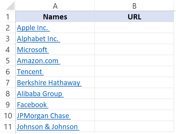
Below is an example where I have the name of companies in one column and their website URL in another column.

Below is the HYPERLINK function to get the result where the text is the company name and it links to the company website.
In the examples so far, we have seen how to create hyperlinks to websites.
But you can also create hyperlinks to worksheets in the same workbook, other workbooks, and files and folders on your hard disk.
Let’s see how it can be done.
Create a Hyperlink to a Worksheet in the Same Workbook
Below are the steps to create a hyperlink to Sheet2 in the same workbook:
- Select the cell in which you want the link
- Enter the text that you want to be hyperlinked. In this example, I have used the text ‘Link to Sheet2’.
- Click the Insert tab.
- Click the links button. This will open the Insert Hyperlink dialog box (You can also use the keyboard shortcut – Control + K).
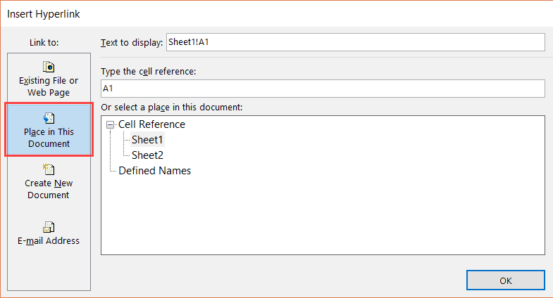
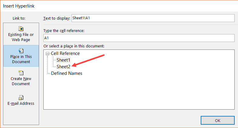
- In the Insert Hyperlink dialog box, select ‘Place in This Document’ option in the left pane.

- Enter the cell which you want to hyperlink (I am going with the default A1).
- Select the sheet that you want to hyperlink (Sheet2 in this case)
- Click OK.

Note: You can also use the same method to create a hyperlink to any cell in the same workbook. For example, if you want to link to a far off cell (say K100), you can do that by using this cell reference in step 6 and selecting the existing sheet in step 7.
You can also use the same method to link to a defined name (named cell or named range). If you have any named ranges (named cells) in the workbook, these would be listed in under the ‘Defined Names’ category in the ‘Insert Hyperlink’ dialog box.
Apart from the dialog box, there is also a function in Excel that allows you to create hyperlinks.
So instead of using the dialog box, you can instead use the HYPERLINK formula to create a link to a cell in another worksheet.
The below formula will do this:
=HYPERLINK("#"&"Sheet2!A1","Link to Sheet2")
Below is how this formula works:
- “#” would tell the formula to refer to the same workbook.
- “Sheet2!A1” tells the formula the cell that should be linked to in the same workbook
- “Link to Sheet2” is the text that appears in the cell.
Create a Hyperlink to a File (in the same or different folders)
You can also use the same method to create hyperlinks to other Excel (and non-Excel) files that are in the same folder or are in other folders.
For example, if you want to open a file with the Test.xlsx which is in the same folder as your current file, you can use the below steps:
- Select the cell in which you want the hyperlink
- Click the Insert tab.
- Click the links button. This will open the Insert Hyperlink dialog box (You can also use the keyboard shortcut – Control + K).
- In the Insert Hyperlink dialog box, select ‘Existing File or Webpage’ option in the left pane.
- Select ‘Current folder’ in the Look in options
- Select the file for which you want to create the hyperlink. Note that you can link to any file type (Excel as well as non-Excel files)

- [Optional] Change the Text to Display name if you want to.
- Click OK.

In case you want to link to a file which is not in the same folder, you can Browse the file and then select it. To Browse the file, click on the folder icon in the Insert Hyperlink dialog box (as shown below).

You can also do this using the HYPERLINK function.
The below formula will create a hyperlink that links to a file in the same folder as the current file:
=HYPERLINK("Test.xlsx","Test File")
In case the file is not in the same folder, you can copy the address of the file and use it as the link_location.
Create a Hyperlink to a Folder
This one also follows the same methodology.
Below are the steps to create a hyperlink to a folder:
- Copy the folder address for which you want to create the hyperlink
- Select the cell in which you want the hyperlink
- Click the Insert tab.
- Click the links button. This will open the Insert Hyperlink dialog box (You can also use the keyboard shortcut – Control + K).
- In the Insert Hyperlink dialog box, paste folder address
- Click OK.

You can also use the HYPERLINK function to create a hyperlink that points to a folder.
For example, the below formula will create a hyperlink to a folder named TEST on the desktop and as soon as you click on the cell with this formula, it will open this folder.
=HYPERLINK("C:UserssumitDesktopTest","Test Folder")
To use this formula, you will have to change the address of the folder to the one you want to link to.
Create Hyperlink to an Email Address
You can also have hyperlinks which open your default email client (such as Outlook) and have the recipients email and the subject line already filled in the send field.
Below are the steps to create an email hyperlink:
- Select the cell in which you want the hyperlink
- Click the Insert tab.
- Click the links button. This will open the Insert Hyperlink dialog box (You can also use the keyboard shortcut – Control + K).
- In the insert dialog box, click on ‘E-mail Address’ in the ‘Link to’ options
- Enter the E-mail address and the Subject line

- [Optional] Enter the text you want to be displayed in the cell.
- Click OK.

Now when you click on the cell which has the hyperlink, it will open your default email client with the email and subject line pre-filled.
You can also do this using the HYPERLINK function.
The below formula will open the default email client and have one email address already pre-filled.
=HYPERLINK("mailto:abc@trumpexcel.com","Send Email")
Note that you need to use mailto: before the email address in the formula. This tells the HYPERLINK function to open the default email client and use the email address that follows.
In case you want to have the subject line as well, you can use the below formula:
=HYPERLINK("mailto:abc@trumpexcel.com,?cc=&bcc=&subject=Excel is Awesome","Generate Email")
In the above formula, I have kept the cc and bcc fields as empty, but you can also these emails if needed.
Here is a detailed guide on how to send emails using the HYPERLINK function.
Remove Hyperlinks
If you only have a few hyperlinks, you can remove these manually, but if you have a lot, you can use a VBA Macro to do this.
Manually Remove Hyperlinks
Below are the steps to remove hyperlinks manually:
- Select the data from which you want to remove hyperlinks.
- Right-click on any of the selected cell.
- Click on the ‘Remove Hyperlink’ option.


The above steps would instantly remove hyperlinks from the selected cells.
In case you want to remove hyperlinks from the entire worksheet, select all the cells and then follow the above steps.
Remove Hyperlinks Using VBA
Below is the VBA code that will remove the hyperlinks from the selected cells:
Sub RemoveAllHyperlinks()
'Code by Sumit Bansal @ trumpexcel.com
Selection.Hyperlinks.Delete
End Sub
If you want to remove all the hyperlinks in the worksheet, you can use the below code:
Sub RemoveAllHyperlinks()
'Code by Sumit Bansal @ trumpexcel.com
ActiveSheet.Hyperlinks.Delete
End Sub
Note that this code will not remove the hyperlinks created using the HYPERLINK function.
You need to add this VBA code in the regular module in the VB Editor.
If you need to remove hyperlinks quite often, you can use the above VBA codes, save it in the Personal Macro Workbook, and add it to your Quick Access Toolbar. This will allow you to remove hyperlinks with a single click and it will be available in all the workbooks on your system.
Here is a detailed guide on how to remove hyperlinks in Excel.
Prevent Excel from Creating Hyperlinks Automatically
For some people, it’s a great feature that Excel automatically converts a URL text to a hyperlink when entered in a cell.
And for some people, it’s an irritation.
If you’re in the latter category, let me show you a way to prevent Excel from automatically creating URLs into hyperlinks.
The reason this happens as there is a setting in Excel that automatically converts ‘Internet and network paths’ into hyperlinks.
Here are the steps to disable this setting in Excel:
- Click the File tab.
- Click on Options.

- In the Excel Options dialog box, click on ‘Proofing’ in the left pane.

- Click on the AutoCorrect Options button.
- In the AutoCorrect dialog box, select the ‘AutoFormat As You Type’ tab.

- Uncheck the option – ‘Internet and network paths with hyperlinks’

- Click OK.
- Close the Excel Options dialog box.


If you’ve completed the following steps, Excel would not automatically turn URLs, email address, and network paths into hyperlinks.
Note that this change is applied to the entire Excel application, and would be applied to all the workbooks that you work with.
Extract Hyperlink URLs (using VBA)
There is no function in Excel that can extract the hyperlink address from a cell.
However, this can be done using the power of VBA.
For example, suppose you have a dataset (as shown below) and you want to extract the hyperlink URL in the adjacent cell.
Let me show you two techniques to extract the hyperlinks from the text in Excel.
Extract Hyperlink in the Adjacent Column
If you want to extract all the hyperlink URLs in one go in an adjacent column, you can so that using the below code:
Sub ExtractHyperLinks()
Dim HypLnk As Hyperlink
For Each HypLnk In Selection.Hyperlinks
    HypLnk.Range.Offset(0, 1).Value = HypLnk.Address
Next HypLnk
End Sub
The above code goes through all the cells in the selection (using the FOR NEXT loop) and extracts the URLs in the adjacent cell.
In case you want to get the hyperlinks in the entire worksheet, you can use the below code:
Sub ExtractHyperLinks()
On Error Resume Next
Dim HypLnk As Hyperlink
For Each HypLnk In ActiveSheet.Hyperlinks
    HypLnk.Range.Offset(0, 1).Value = HypLnk.Address
Next HypLnk
End Sub
Note that the above codes wouldn’t work for hyperlinks created using the HYPERLINK function.
Extract Hyperlink Using a Formula (created with VBA)
The above code works well when you want to get the hyperlinks from a dataset in one go.
But if you have a list of hyperlinks that keeps expanding, you can create a User Defined Function/formula in VBA.
This will allow you to quickly use the cell as the input argument and it will return the hyperlink address in that cell.
Below is the code that will create a UDF for getting the hyperlinks:
Function GetHLink(rng As Range) As String
    If rng(1).Hyperlinks.Count <> 1 Then
        GetHLink = ""
    Else
        GetHLink = rng.Hyperlinks(1).Address
    End If
End Function
Note that this wouldn’t work with Hyperlinks created using the HYPERLINK function.
Also, in case you select a range of cells (instead of a single cell), this formula will return the hyperlink in the first cell only.
Find Hyperlinks with Specific Text
If you’re working with a huge dataset that has a lot of hyperlinks in it, it could be a challenge when you want to find the ones that have a specific text in it.
For example, suppose I have a dataset as shown below and I want to find all the cells with hyperlinks that have the text 2019 in it and change it to 2020.

And no.. doing this manually is not an option.
You can do that using a wonderful feature in Excel – Find and Replace.
With this, you can quickly find and select all the cells that have a hyperlink and then change the text 2019 with 2020.
Below are the steps to select all the cells with a hyperlink and the text 2019:
- Select the range in which you want to find the cells with hyperlinks with 2019. In case you want to find in the entire worksheet, select the entire worksheet (click on the small triangle at the top left).
- Click the Home tab.

- In the Editing group, click on Find and Select

- In the drop-down, click on Replace. This will open the Find and Replace dialog box.

- In the Find and Replace dialog box, click on the Options button.This will show more options in the dialog box.

- In the ‘Find What’ options, click on the little downward pointing arrow in the Format button (as shown below).

- Click on the ‘Choose Format From Cell’. This will turn your cursor into a plus icon with a format picker icon.

- Select any cell which has a hyperlink in it. You will notice that the Format gets visible in the box on the left of the Format button. This indicates that the format of the cell you selected has been picked up.
- Enter 2019 in the ‘Find What’ field and 2020 in the ‘Replace with’ field.
- Click on the Replace All button.


In the above data, it will change the text of four cells that have the text 2019 in it and also has a hyperlink.
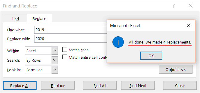
You can also use this technique to find all the cells with hyperlinks and get a list of it. To do this, instead of clicking on Replace All, click on the Find All button. This will instantly give you a list of all the cell address that has hyperlinks (or hyperlinks with specific text depending on what you’ve searched for).
Note: This technique works as Excel is able to identify the formatting of the cell that you select and use that as a criterion to find cells. So if you’re finding hyperlinks, make sure you select a cell that has the same kind of formatting. If you select a cell that has a background color or any text formatting, it may not find all the correct cells.
Selecting a Cell that has a Hyperlink in Excel
While Hyperlinks are useful, there are a few things about it that irritate me.
For example, if you want to select a cell that has a hyperlink in it, Excel would automatically open your default web browser and try to open this URL.
Another irritating thing about it is that sometimes when you have a cell that has a hyperlink in it, it makes the entire cell clickable. So even if you’re clicking on the hyperlinked text directly, it still opens the browser and the URL of the text.
So let me quickly show you how to get rid of these minor irritants.
Select the Cell (without opening the URL)
This is a simple trick.
When you hover the cursor over a cell that has a hyperlink in it, you’ll notice the hand icon (which indicates if you click on it, Excel will open the URL in a browser)
![]()
Click the cell anyway and hold the left button of the mouse.
After a second, you’ll notice that the hand cursor icon changes into the plus icon, and now when you leave it, Excel will not open the URL.
![]()
Instead, it would select the cell.
Now, you can make any changes in the cell you want.
Neat trick… right?
Select a Cell by clicking on the blank space in the cell
This is another thing that might drive you nuts.
When there is a cell with the hyperlink in it as well as some blank space, and you click on the blank space, it still opens the hyperlink.
![]()
Here is a quick fix.
This happens when these cells have the wrap text enabled.
If you disable wrap text for these cells, you will be able to click on the white space on the right of the hyperlink without opening this link.
Some Practical Example of Using Hyperlink
There are useful things you can do when working with hyperlinks in Excel.
In this section, I am going to cover some examples that you may find useful and can use in your day-to-day work.
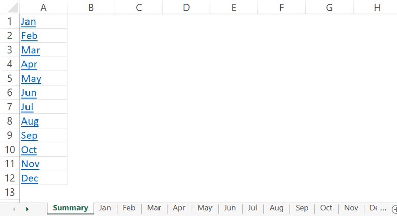
Example 1 – Create an Index of All Sheets in the Workbook
If you have a workbook with a lot of sheets, you can use a VBA code to quickly create a list of the worksheets and hyperlink these to the sheets.
This could be useful when you have 12-month data in 12 different worksheets and want to create one index sheet that links to all these monthly data worksheets.
Below is the code that will do this:
Sub CreateSummary()
'Created by Sumit Bansal of trumpexcel.com
'This code can be used to create summary worksheet with hyperlinks
Dim x As Worksheet
Dim Counter As Integer
Counter = 0
For Each x In Worksheets
Counter = Counter + 1
If Counter = 1 Then GoTo Donothing
    With ActiveCell
        .Value = x.Name
        .Hyperlinks.Add ActiveCell, "", x.Name & "!A1", TextToDisplay:=x.Name, ScreenTip:="Click here to go to the Worksheet"
        With Worksheets(Counter)
            .Range("A1").Value = "Back to " & ActiveSheet.Name
            .Hyperlinks.Add Sheets(x.Name).Range("A1"), "", _
            "'" & ActiveSheet.Name & "'" & "!" & ActiveCell.Address, _
            ScreenTip:="Return to " & ActiveSheet.Name
        End With
    End With
ActiveCell.Offset(1, 0).Select
Donothing:
Next x
End Sub
You can place this code in the regular module in the workbook (in VB Editor)
This code also adds a link to the summary sheet in cell A1 of all the worksheets. In case you don’t want that, you can remove that part from the code.
You can read more about this example here.
Note: This code works when you have the sheet (in which you want the summary of all the worksheets with links) at the beginning. In case it’s not at the beginning, this may not give the right results).
Example 2 – Create Dynamic Hyperlinks
In most cases, when you click on a hyperlink in a cell in Excel, it will take you to a URL or to a cell, file or folder. Normally, these are static URLs which means that a hyperlink will take you to a specific predefined URL/location only.
But you can also use a little bit for Excel formula trickery to create dynamic hyperlinks.
By dynamic hyperlinks, I mean links that are dependent on a user selection and change accordingly.
For example, in the below example, I want the hyperlink in cell E2 to point to the company website based on the drop-down list selected by the user (in cell D2).

This can be done using the below formula in cell E2:
=HYPERLINK(VLOOKUP(D2,$A$2:$B$6,2,0), "Click here")
The above formula uses the VLOOKUP function to fetch the URL from the table on the left. The HYPERLINK function then uses this URL to create a hyperlink in the cell with the text – ‘Click here’.
When you change the selection using the drop-down list, the VLOOKUP result will change and would accordingly link to the selected company’s website.
This could be a useful technique when you’re creating a dashboard in Excel. You can make the hyperlinks dynamic depending on the user selection (which could be a drop-down list or a checkbox or a radio button).
Here is a more detailed article of using Dynamic Hyperlinks in Excel.
Example 3 – Quickly Generate Simple Emails Using Hyperlink Function
As I mentioned in this article earlier, you can use the HYPERLINK function to quickly create simple emails (with pre-filled recipient’s emails and the subject line).
Single Recipient Email Id
=HYPERLINK("mailto:abc@trumpexcel.com","Generate Email")
This would open your default email client with the email id abc@trumpexcel.com in the ‘To’ field.
Multiple Recipients Email Id
=HYPERLINK("mailto:abc@trumpexcel.com,def@trumpexcel.com","Generate Email")
For sending the email to multiple recipients, use a comma to separate email ids. This would open the default email client with all the email ids in the ‘To’ field.
Add Recipients in CC and BCC List
=HYPERLINK("mailto:abc@trumpexcel.com,def@trumpexcel.com?cc=123@trumpexcel.com&bcc=456@trumpexcel.com","Generate Email")
To add recipients to CC and BCC list, use question mark ‘?’ when ‘mailto’ argument ends, and join CC and BCC with ‘&’. When you click on the link in excel, it would have the first 2 ids in ‘To’ field, 123@trumpexcel.com in ‘CC’ field and 456@trumpexcel.com in the ‘BCC’ field.
Add Subject Line
=HYPERLINK("mailto:abc@trumpexcel.com,def@trumpexcel.com?cc=123@trumpexcel.com&bcc=456@trumpexcel.com&subject=Excel is Awesome","Generate Email")
You can add a subject line by using the &Subject code. In this case, this would add ‘Excel is Awesome’ in the ‘Subject’ field.
Add Single Line Message in Body
=HYPERLINK("mailto:abc@trumpexcel.com,def@trumpexcel.com?cc=123@trumpexcel.com&bcc=456@trumpexcel.com&subject=Excel is Awesome&body=I love Excel","Email Trump Excel")
This would add a single line ‘I love Excel’ to the email message body.
Add Multiple Lines Message in Body
=HYPERLINK("mailto:abc@trumpexcel.com,def@trumpexcel.com?cc=123@trumpexcel.com&bcc=456@trumpexcel.com&subject=Excel is Awesome&body=I love Excel.%0AExcel is Awesome","Generate Email")
To add multiple lines in the body you need to separate each line with %0A. If you wish to introduce two line breaks, add %0A twice, and so on.
Here is a detailed article on how to send emails from Excel.
Hope you found this article useful.
Let me know your thoughts in the comments section.
You May Also Like the Following Excel Tutorials:
- Excel AutoCorrect
- How to Find External Links and References in Excel
- 100+ Excel Interview Questions & Answers
- Excel Text to Columns
- Excel Sparklines
Skip to content
В статье объясняются основы функции ГИПЕРССЫЛКА в Excel и приводятся несколько советов и примеров формул для ее наиболее эффективного использования.
Существует множество способов создать гиперссылку в Excel. Чтобы сделать ссылку на определенную веб-страницу, вы можете просто ввести ее URL-адрес в ячейку, нажать Enter, и Microsoft Excel автоматически преобразует запись в интерактивную гиперссылку.
Чтобы создать ссылку на другой рабочий лист или определенное место в другом файле Excel, вы можете использовать контекстное меню «Гиперссылка» или комбинацию клавиш Ctrl + К.
Но если вы хотите вставить на рабочий лист много одинаковых или похожих ссылок, то самый быстрый способ — использовать формулу гиперссылки, которая упрощает создание, копирование и редактирование гиперссылок в Excel.
Функция ГИПЕРССЫЛКА в Excel — синтаксис и способы использования
Функция ГИПЕРССЫЛКА в Excel используется для создания ссылки, которая направляет пользователя в указанное место в том же документе или открывает другой документ или веб-страницу. Используя формулу гиперссылки, вы можете ссылаться на:
- Определенное место, например ячейку или именованный диапазон в файле Excel (на существующем листе, или на другом листе, или в другой книге).
- Документ Word, презентацию PowerPoint или другой документ, хранящийся на жестком диске, в локальной сети или в Интернете.
- Закладка в документе Word.
- Веб-страница в Интернете.
- Адрес электронной почты для создания нового сообщения.
Эта функция доступна во всех версиях Excel для Office 365, Excel от 2019 до 2000. В Excel Online функцию ГИПЕРССЫЛКА можно использовать только для веб-адреса (URL).
Синтаксис функции ГИПЕРССЫЛКА следующий:
ГИПЕРССЫЛКА(адрес ; [имя])
Где:
- адрес (обязательно) — по которому необходимо перейти.
Он может быть представлен как ссылка на ячейку, содержащую ссылку, или же быть текстовой строкой, заключенной в кавычки, которая содержит путь к файлу, хранящемуся на локальном диске, или URL-адресом в Интернете.
Если указанный путь ссылки не существует или не работает, формула гиперссылки выдаст ошибку при попытке кликнуть по ней.
- имя (необязательно) — это пояснительный текст, который будет отображаться в ячейке. Чтобы было понятно, куда ведёт ссылка. Если опущено, то адрес из первого аргумента отображается как текст ссылки.
Этот аргумент может быть представлен в виде числа, текстовой строки, заключенной в кавычки, или ссылки на ячейку, содержащую нужный текст.
Щелчок по ячейке с формулой гиперссылки открывает файл или веб-страницу, указанную в аргументе адрес.
Ниже вы можете увидеть простейший пример формулы гиперссылки Excel, где A2 содержит имя, а B2 содержит адрес:
=ГИПЕРССЫЛКА(B2; A2)
Результат может выглядеть примерно так:

Ниже вы можете ознакомиться с примерами формул, демонстрирующими другие варианты использования функции ГИПЕРССЫЛКА в Excel.
Как использовать ГИПЕРССЫЛКА в Excel — примеры формул
Переходя от теории к практике, давайте посмотрим, как вы можете использовать функцию ГИПЕРССЫЛКА, чтобы открывать различные документы прямо из ваших рабочих таблиц. Мы также обсудим более сложную формулу, в которой она используется в сочетании с несколькими другими функциями для выполнения сложной задачи.
Функция Excel ГИПЕРССЫЛКА позволяет вам создавать ссылки нескольких различных типов, в зависимости от того, какое значение вы указываете в аргументе адрес. Рассмотрим, как создавать ссылки на листы, файлы, веб-страницы и другие элементы.
Гиперссылка на другой рабочий лист
Чтобы вставить гиперссылку на другой лист в той же книге, укажите перед именем целевого листа знак решетки (#), после него – восклицательный знак и имя целевой ячейки, например:
=ГИПЕРССЫЛКА(«#Лист1!A1″;»Лист1»)
Приведенная выше формула создает гиперссылку с текстом перехода «Лист1», которая открывает Лист1 из текущей книги и устанавливает курсор в A1.
Если имя рабочего листа содержит пробелы или неалфавитные символы, оно обязательно должно быть заключено в одинарные кавычки, например:
=ГИПЕРССЫЛКА(«#‘Лист 1‘!A1″;»Лист 1″)
Таким же образом можно создать гиперссылку на другую ячейку того же листа. Например, чтобы вставить гиперссылку, которая приведет вас к ячейке A1 на том же листе, используйте формулу, подобную этой:
=ГИПЕРССЫЛКА(«#A1″;»Перейти к ячейке А1»)
Гиперссылка на другую книгу
Чтобы создать гиперссылку на другую книгу, необходимо указать полный путь к целевой книге в следующем формате:
«Диск:ПапкаКнига.xlsx»
Например:
=ГИПЕРССЫЛКА(«C:ГиперссылкиКнига2.xlsx»;»Книга2″)
Чтобы перейти на конкретный лист и даже в конкретную ячейку, используйте этот формат:
«[Диск:ПапкаКнига.xlsx]Лист!Ячейка»
Например, чтобы добавить гиперссылку с названием «Книга3», которая открывает Лист2 в Книга2, хранящейся в папке Гиперссылки на диске С, попробуйте следующую формулу:
=ГИПЕРССЫЛКА(«[C:ГиперссылкиКнига2.xlsx]Лист2!A1″;»Книга2 Лист2 А1»)
В данном случае вы используете так называемую абсолютную гиперссылку, в которой целевой адрес абсолютно зафиксирован.
Если вы планируете в ближайшее время переместить свои файлы в другое место, более целесообразно создать относительную гиперссылку примерно так:
=ГИПЕРССЫЛКА(«ГиперссылкиКнига2.xlsx»;»Книга2″)
И раз об этом зашел разговор, остановимся подробнее на абсолютных и относительных гиперссылках.
Абсолютные и относительные гиперссылки в Excel
Microsoft Excel поддерживает два типа ссылок: абсолютные и относительные, в зависимости от того, указываете ли вы полный или частичный адрес.
Абсолютная гиперссылка содержит полный адрес, включая протокол и доменное имя для URL-адресов, а также полный путь и имя файла для документов. Например:
Абсолютный URL: https://mister-office.ru/funktsii-excel/function-if-excel-primery.html
В Интернете общепринятой практикой является использование относительных URL-адресов. В гиперссылках Excel всегда следует указывать полные URL-адреса веб-страниц . Однако Microsoft Excel может понимать URL-адреса без протокола.
Например, если вы введете «www.mister-office.ru» в ячейку, Excel автоматически добавит протокол «http» по умолчанию и преобразует его в гиперссылку, по которой вы можете перейти.
Со ссылками на файлы немного сложнее.
При создании ссылок на файлы Excel или другие документы, хранящиеся на вашем компьютере, вы можете использовать как абсолютные, так и относительные адреса.
Абсолютная ссылка на файл Excel: C:Excel filesSource DataBook1.xlsx
В случае абсолютной гиперссылки путь к цели указан совершенно явно и точно и должен быть обновлен каждый раз, когда файл перемещается в другое место.
Относительная гиперссылка содержит частичный адрес. Например:
Пример относительной ссылки на файл Excel: Source dataBook1.xlsx
Относительная гиперссылка — это гиперссылка, которая содержит целевой адрес относительно адреса файла, в котором она записана.
В относительной гиперссылке отсутствующая часть пути к файлу относится к расположению активной книги. Основное преимущество этого подхода заключается в том, что вам не нужно редактировать адрес ссылки при перемещении файлов в другое место.
Например, если ваша активная книга и целевая книга находятся на диске C, а затем вы перемещаете их на диск D, относительные гиперссылки будут продолжать работать до тех пор, пока относительный путь к целевому файлу остается неизменным.
Гиперссылка на именованный диапазон
Если вы создаете гиперссылку на именованный диапазон на рабочем листе, укажите полный путь к целевому имени:
«[Диск:ПапкаКнига.xlsx]Лист!Имя»
Например, чтобы вставить ссылку на диапазон с именем «Диапазон_данных», хранящийся на Лист2 в Книга2, используйте следующую формулу:
=ГИПЕРССЫЛКА(«[C:ГиперссылкиКнига2.xlsx]Лист2!Диапазон_данных»;»Книга2 Лист2 Диапазон данных»)
Если вы ссылаетесь на именованный диапазон уровня рабочей книги, имя листа указывать не нужно, например:
=ГИПЕРССЫЛКА(«[C:ГиперссылкиКнига2.xlsx]Диапазон_данных_1″;»Диапазон данных 1»)
Гиперссылка для открытия файла, хранящегося на жестком диске
Чтобы создать ссылку, открывающую другой документ, укажите полный путь к этому документу в следующем формате:
«Диск:Папкаимя_файла.расширение»
Например, чтобы открыть документ Word с именем Прайс—лист, который хранится в папке Word files на диске D, используйте следующую формулу:
=ГИПЕРССЫЛКА(«D:Word filesПрайс-лист.docx»;»Прайс лист»)
Гиперссылка на закладку в документе Word
Чтобы сделать гиперссылку на определенное место в документе Word, заключите путь к документу в [квадратные скобки] и используйте закладку , чтобы определить место, к которому вы хотите перейти.
Например, следующая формула добавляет гиперссылку на закладку с именем Таблица_скидок в файле Цены.docx :
=ГИПЕРССЫЛКА(«[C:ГиперссылкиЦены.docx]Таблица_скидок»;»Скидки»)
Гиперссылка на файл на сетевом диске
Чтобы открыть файл, хранящийся в вашей локальной сети, укажите путь к этому файлу в формате универсального соглашения об именах (UNC), в котором перед именем сервера используется двойная обратная косая черта, например:
«\имя_серверапапкаимя_файла.расширение»
Приведенная ниже формула создает гиперссылку под названием « Прайс на сервере», которая открывает книгу «Прайс-лист.xlsx », хранящуюся на SERVER1 в папке Alex :
=ГИПЕРССЫЛКА(«\SERVERAlexПрайс-лист.xlsx»;»Прайс на сервере»)
Чтобы открыть сетевой файл Excel на определенном листе, заключите путь к файлу в [квадратные скобки] и напишите далее имя листа, восклицательный знак (!) и ячейку, на которую указывает ссылка:
=ГИПЕРССЫЛКА(«[\SERVERAlexПрайс-лист.xlsx]Лист1!А1″;»Прайс Лист1 на сервере»)
Гиперссылка на веб-страницу
Чтобы создать гиперссылку на веб-страницу в Интернете, укажите ее URL-адрес, заключенный в кавычки, например:
=ГИПЕРССЫЛКА(«https://www.mister-office.ru»4; «Перейти на Мистер Офис»)
Приведенная выше формула вставляет гиперссылку под названием «Перейти на Мистер Офис», которая открывает домашнюю страницу нашего веб-сайта.
Гиперссылка для отправки электронного письма
Чтобы создать по клику на ячейку новое сообщение для определенного получателя, укажите адрес электронной почты в следующем формате:
«mailto:email_address»
Например:
=ГИПЕРССЫЛКА(«mailto:alex@mister-office.ru»;»Отправить email»)
Приведенная выше формула добавляет гиперссылку под названием « Отправить email», и нажатие на нее создает новое почтовое сообщение.
Искать значение и создать гиперссылку на первое совпадение
При работе с большими наборами данных вы часто можете оказаться в ситуации, когда вам нужно найти конкретное значение и вернуть соответствующие данные из другого столбца. Для этого вы используете либо функцию ВПР, либо более мощную комбинацию ПОИСКПОЗ ИНДЕКС .
Но что, если вы хотите не только получить соответствующее значение, но и перейти к позиции этого значения в исходном наборе данных, чтобы просмотреть другие детали в той же строке? Это можно сделать с помощью функции ГИПЕРССЫЛКА Excel с некоторой помощью функций ЯЧЕЙКА, ИНДЕКС и ПОИСКПОЗ.
Общая формула для создания гиперссылки на первое совпадение выглядит следующим образом:
ГИПЕРССЫЛКА(«#»&ЯЧЕЙКА(«адрес»; ИНДЕКС( массив; ПОИСКПОЗ ( искомое_значение ; диапазон_поиска ;0))), ИНДЕКС( массив; ПОИСКПОЗ ( искомое_значение; диапазон_поиска ;0)))
Чтобы увидеть эту формулу в действии, рассмотрим следующий пример. Предположим, у вас есть список продавцов в столбце A и проданных товаров в столбце C. Вы хотите найти первый товар, проданный определенным продавцом, и создать гиперссылку на какую-либо ячейку в этой строке, чтобы вы могли перейти туда просмотреть все другие подробности, связанные именно с этим конкретным заказом.
С искомым значением в ячейке F2, списком продавцов (диапазон поиска) в A2:A10 и списком товаров (массив данных) в C2:C10 формула принимает следующий вид:
=ГИПЕРССЫЛКА(«#»&@ЯЧЕЙКА(«address»; ИНДЕКС($C$2:$C$10; ПОИСКПОЗ($E2;$A$2:$A$10;0))); ИНДЕКС($C$2:$C$10; ПОИСКПОЗ($E2;$A$2:$A$10;0)))
Как видно на скриншоте ниже, формула извлекает найденное значение и преобразует его в интерактивную гиперссылку, которая направляет пользователя к позиции первого совпадения в исходном наборе данных.

Если вы работаете с длинными строками данных, то может быть удобнее, чтобы гиперссылка указывала на первую ячейку в строке, где найдено совпадение. Для этого вы просто указываете другой массив в первой комбинации ИНДЕКС ПОИСКПОЗ – столбец A (в этом примере $A$2:$A$10):
=ГИПЕРССЫЛКА(«#»&@ЯЧЕЙКА(«address»; ИНДЕКС($A$2:$A$10; ПОИСКПОЗ($E2;$A$2:$A$10;0))); ИНДЕКС($C$2:$C$10; ПОИСКПОЗ($E2;$A$2:$A$10;0)))
Эта формула приведет вас к первой ячейке в строке с найденным товаром, который в нашем случае был обнаружен в третьей ячейке строки:

Примечание. Обратите внимание на использование абсолютных ссылок на ячейки для используемых диапазонов. Это важно, если вы планируете вставить более одной гиперссылки, скопировав формулу вниз по столбцу.
Как редактировать несколько гиперссылок одновременно
Как упоминалось в начале статьи, одним из наиболее полезных преимуществ гиперссылок на основе формул является возможность редактирования сразу нескольких формул гиперссылок за один приём с помощью функции Excel «Заменить все».
Предположим, вы хотите заменить старый URL-адрес своей компании (old-website.com) новым (new-website.com) во всех гиперссылках на текущем листе или во всей книге. Чтобы это сделать, выполните шаги, описанные ниже:
- Нажмите клавиши
Ctrl + Н, чтобы открыть вкладку «Заменить» диалогового окна «Найти и заменить». - В поле «Найти» введите текст, который вы хотите изменить (в данном примере — «old-website.com»). В поле Заменить на введите новый текст («new-website.com» в данном примере).
- В правой части диалогового окна нажмите кнопку Параметры.
- В вкладке Параметры выберите Лист или Книга в зависимости от того, хотите ли вы изменить гиперссылки только на текущем листе или на всех листах текущей книги.
- Там же в параметрах в пункте Искать в выберите Формулы.
- В качестве дополнительной меры предосторожности сначала нажмите кнопку «Найти все», и Excel отобразит список всех формул, содержащих искомый текст:

- Просмотрите результаты поиска, чтобы убедиться, что вы хотите изменить все найденные формулы. Если вы это сделаете, перейдите к следующему шагу, в противном случае уточните поиск.
- Нажмите кнопку «Заменить все». Excel заменит указанный текст во всех найденных гиперссылках и сообщит, сколько изменений было внесено.
- Нажмите кнопку Закрыть. Готово!
Аналогичным образом вы можете одновременно редактировать текст ссылки (второй параметр) во всех формулах гиперссылки. При этом убедитесь, что заменяемый текст в аргументе имя нигде не появляется в адресе, чтобы не нарушить формулы.
ГИПЕРССЫЛКА Excel не работает — причины и решения
Самая распространенная причина, по которой формула гиперссылки не работает (и первое, что вы должны проверить!) — это несуществующий или неверный путь в аргументе адрес. Если это не так, проверьте следующие две вещи:
- Если место назначения ссылки не открывается при нажатии на гиперссылку, убедитесь, что расположение ссылки указано в правильном формате. Примеры формул для создания различных типов гиперссылок можно найти выше.
- Если вместо текста ссылки появится ошибка типа ЗНАЧ! или N/A, скорее всего, проблема связана с аргументом имя вашей формулы гиперссылки.
Как правило, такие ошибки возникают, когда имя возвращается какой-либо другой функцией (функциями), например, в нашем ВПР и гиперссылке на первое совпадение. В этом случае в ячейке формулы появится ошибка #Н/Д, если искомое значение не будет найдено в таблице поиска. Чтобы предотвратить такие ошибки, вы можете рассмотреть возможность использования функции ЕСЛИОШИБКА для отображения пустой строки или некоторого понятного для пользователя текста вместо значения ошибки.
Вот как можно создавать различные ссылки с помощью функции Excel ГИПЕРССЫЛКА.
Другие статьи по теме:
 Как удалить сразу несколько гиперссылок — В этой короткой статье я покажу вам, как можно быстро удалить сразу все нежелательные гиперссылки с рабочего листа Excel и предотвратить их появление в будущем. Решение работает во всех версиях Excel,… Гиперссылка в Excel: как сделать, изменить, удалить — В статье разъясняется, как сделать гиперссылку в Excel, используя 3 разных метода. Вы узнаете, как вставлять, изменять и удалять гиперссылки на рабочих листах, а также исправлять неработающие ссылки. Гиперссылки широко используются…
  Как использовать функцию ДВССЫЛ – примеры формул — В этой статье объясняется синтаксис функции ДВССЫЛ, основные способы ее использования и приводится ряд примеров формул, демонстрирующих использование ДВССЫЛ в Excel. В Microsoft Excel существует множество функций, некоторые из которых…
If you need quick access to a file outside of Excel, you can insert or create excel hyperlinks in Excel worksheets on a web page or in another file. Excel also allows you to insert excel hyperlinks in specific chart elements.

In this article, you’ll learn how to create hyperlinks pointing to different destinations in Excel using different methods (including some useful tips and examples). As a bonus, you’ll also learn how to add hyperlinks in Google Sheets.
Here are four ways to create an Excel hyperlink:
- Type the URL
- Use the Insert Hyperlink command
- Drag and drop a Link
- Use the HYPERLINK function
These methods can help you create a link in Excel that points to different destinations, including:
- Link to a new file.
- Link to an existing file or web page.
- Link to a specific location in a workbook.
- Create a custom link using the HYPERLINK function.
- Link to an email address.
- Create an external reference link to worksheet data on the web.
- Link without activating the ling
Note: Excel also allows you to change a hyperlink, change the appearance of a link in a text, change the graphic or text in a link, copy or move a link and set the base address of the links in a workbook.
1] Type the URL
You can create a hyperlink that points to a particular website, document or image, etc., on the web.
If you type a valid website address in a Worksheet cell and press Enter, Excel will automatically create a hyperlink
For example,
- In cell B3 below, type the address of the Contextures website: https://www.softwarekeep.com.
- Press Enter


You typed changes to a hyperlink, and you can click the link to go to the Softwarekeep website.
2] Use the Insert Hyperlink command
Excel has the built-in ‘Insert hyperlink’ command that allows you to insert hyperlinks as you please. Use the following steps to insert a hyperlink using this command:
- On a worksheet, select the cell where you want to create a hyperlink.
- In the Excel ribbon, click the Insert tab, then select Link or Hyperlink command.
 or
or 


Alternatively, you can also right-click the cell and then select Link/hyperlink on the shortcut menu or use the Ctrl+K shortcut.
- Under the Display Text box, type the text that you want to use to represent the link.
- Now, in the Insert Hyperlink dialog box, choose the link type on the left pane, i.e.
- Existing file or Web Page
- Place in This Document
- Create New Document
- E-mail Address


Create a hyperlink to the Existing File or Web Page
You will use this option to create a hyperlink that connects to another Excel file or directs you to a web page. Use the following steps:
- In the Link To list, click on an Existing File or Web Page on your PC (use the Look in the drop-down list, if necessary).

- Use the folder navigation to find and select the existing file you need to link to.

- OR, type a URL in the address box to link to a web page.

- The result will look like this:


Create a hyperlink: Place in this Document.
The ‘Place in this document option allows you to link to a cell in the same spreadsheet.
In a large spreadsheet, it can be essential to have a table of contents or create a link to find a quick way to get from one section to another. To do this, link a cell to another in the same spreadsheet.
To do that:
- Press Ctrl + K to bring up the Insert Hyperlink dialog.
- In the left pane, select Place in This Document:
- Select a sheet/place in the Or select a place in this document field.
- Type the cell reference:
- Click Ok.


Link to a different workbook
You can easily link to a different spreadsheet as you can link within one.
- Press Ctrl + K to open up the links dialog.
- Select the Existing File or Web Page on the left pane.
- Use the file explorer to find the file you want to link to:
- Click Ok.

Create a Link to a new file: Create New Document
Use the following steps to create a link on a new file. You will use the create New Document option to do this.
- On a worksheet, click the cell where you want to create a link.
- You can also select an object, such as a picture or an element in a chart, that you want to use to represent the link.
- Go to the Insert tab in the Links group, click the Link/Hyperlink button.
- Or right-click the cell or graphic and then click Link/Hyperlink on the shortcut menu.
- Or press Ctrl+K.
- Under Link/Hyperlink, click Create New Document.
- In the Name of new document box, type a name for the new file.Tip: To specify a location other than the one shown under Full path, you can type the new location preceding the name in the Name of new document box, or you can click Change to select the location that you want and then click OK.
- Under When to edit, click Edit the new document later or Edit the new document now to specify when you want to open the new file for editing.
- In the Text to display box, type the text that you want to use to represent the link.

Note: You can choose to add/display helpful information when you rest the pointer on the link. For this, click the ScreenTip then type the text that you want in the ScreenTip text box, and then click OK.
Create hyperlink to an email address
Excel allows you to create a link to an email address.
When you click a link to an email address, your email program automatically starts and creates an email message with the correct address in the To box, provided that you have an email program installed.
- On a worksheet, click the cell where you want to create a link.
- You can also select an object, such as a picture or an element in a chart, that you want to use to represent the link.
- Go to the Insert tab > then the Links group > click the Link/Hyperlink button.
- Or right-click the cell or object and then click Hyperlink/Link on the shortcut menu.
- Or press Ctrl+K.
- Now, under Link to, click Email Address.
- Type the email address that you want in the E-mail address box.
- Type the subject of the email message in the Subject box.
Note: Some web browsers and email programs may not recognize the subject line. - Type the email text you want to represent the link in the Text to display box.
- If you want to display helpful information when you rest the pointer on the link, click ScreenTip, type the text that you want in the ScreenTip text box
- Click OK.


3] Create Hyperlinks with Drag and Drop
The drag and drop method is the quickest way to create hyperlinks within an Excel file.
For instance, you can create a table of contents sheet (TOC), in a workbook, with links to other sections of the document (or sheets).
Follow these steps to create drag and drop hyperlinks:
- Make sure your workbook is saved. This technique won’t work in a new workbook, that hasn’t been saved.
- Click on a cell that you want to link to. This is the cell you’re going to drag to another sheet, where you want to create a hyperlink.
- Point to the cell’s border, and press the right mouse button.
- To drag the cell to another sheet, press the Alt key, and drag the cell onto the other sheet’s tab.

- Once the other sheet is activated, release the Alt key.
- Now, drag to the cell where you want the hyperlink.
- Release the right mouse button.
- In the popup menu, click Create Hyperlink Here.

- Now, you will see a hyperlink in the cell, with the text from the original cell.


4] Use the Excel HYPERLINK function
Another way to insert a link or create hyperlink in Excel is through the Excel HYPERLINK Function.
Through the HYPERLINK function, you can create a link that opens a document that is stored on a network server, an intranet, or the Internet. When you click the cell that contains the HYPERLINK function, Excel opens the file that is stored at the location of the link.
Here’s the syntax of the Excel HYPERLINK function
=HYPERLINK(link_location, [friendly_name])
Where:
- link_location: can be a path to a file or folder, the URL of a web page, or a place in a document (such as a specific cell or named range in an Excel worksheet or workbook).
- [friendly_name]: is an optional argument. This is the text that you want in the cell that has the hyperlink. In case you omit this argument, it will use the link_location text string as the friendly name.
Here are HYPERLINK Function examples:
Link to cells in external spreadsheets
You can use the HYPERLINK function to link to specific cells in external spreadsheets. Here’s how that looks:
=HYPERLINK(“[name of the spreadsheet]cell reference”, “friendly name”)
Link to Worksheet in a Shared Internet
This example (below) opens a worksheet named Budget Report.xls, which is stored on the Internet at the location named example.softwarekeep.com/report and displays the text «Click for report»:
=HYPERLINK(«http://example.softwarekeep.com/report/budget report.xls», «Click for report»)
In the next example, you can create a link to cell F10 on the worksheet named SoftwareKeep.Windows in the workbook Budget Report.xls, which is stored on the Internet at the location named example.softwarekeep.com/report.
The cell on the worksheet that contains the link displays the contents of cell D1 as the jump text. Here’s how it appears:
=HYPERLINK(«[http://example.softwarekeep.com/report/budget report.xls]SoftwareKeep.Windows!F10», D1)
Link Within the Same File
Use the HYPERLINK function to create a link to a cell or range somewhere within the current workbook. When doing this, the trick is to add a pound sign (#) at the start of the address.
Here are examples of HYPERLINK formulas within the same workbook:
Type the Address
Start with a #, then type the sheet name and cell reference.
Optional — Type a friendly name, such as «Budget» to appear in the cell:
=HYPERLINK(«#Sheet2!B2″,»Budget»)
Use Cell References
Use the & operator to create a link location.
In this example, the sheet name is in cell B3, the cell address is in C9, and the friendly name is in cell D7.
=HYPERLINK(«#»&»‘» & B3 & «‘!» & C9,D7)
Type a Range Name
For a link to a workbook-level named range in the same workbook, you will use the range name as the link location. Here’s how to do it:
=HYPERLINK(«#StartCell»,»StartCell»)
Final Thoughts
Creating hyperlinks in Excel documents is a very useful skill to know. And when you can tweak the link creation using different methods, you can not only make your work look nice, but provide useful links that point to more resources for your users. This is a skill that really comes in handy!
One more thing
First, we hope you enjoyed reading this article and you’ve learned how to create hyperlinks in Excel. We have tons of more content in Excel and other tips and tricks in our Help Center that can help you improve your skills and productivity.
Second, If you want to be the first to receive our daily tips and tricks and other guides, sign up to our newsletter. You will also receive promotions, deals, and discounts to get our products for the best price.
You may also like
> How To Use Excel Round Down Function
> How To Calculate Coefficient of Variation in Excel
> How To Use the Excel Data Analysis ToolPak
> How To Calculate a P-Value in Excel
> How to Edit Legend in Excel