
Enter data manually in worksheet cells
Excel for Microsoft 365 Excel 2021 Excel 2019 Excel 2016 Excel 2013 Excel 2010 Excel 2007 More…Less
You have several options when you want to enter data manually in Excel. You can enter data in one cell, in several cells at the same time, or on more than one worksheet at once. The data that you enter can be numbers, text, dates, or times. You can format the data in a variety of ways. And, there are several settings that you can adjust to make data entry easier for you.
This topic does not explain how to use a data form to enter data in worksheet. For more information about working with data forms, see Add, edit, find, and delete rows by using a data form.
Important: If you can’t enter or edit data in a worksheet, it might have been protected by you or someone else to prevent data from being changed accidentally. On a protected worksheet, you can select cells to view the data, but you won’t be able to type information in cells that are locked. In most cases, you should not remove the protection from a worksheet unless you have permission to do so from the person who created it. To unprotect a worksheet, click Unprotect Sheet in the Changes group on the Review tab. If a password was set when the worksheet protection was applied, you must first type that password to unprotect the worksheet.
-
On the worksheet, click a cell.
-
Type the numbers or text that you want to enter, and then press ENTER or TAB.
To enter data on a new line within a cell, enter a line break by pressing ALT+ENTER.
-
On the File tab, click Options.
In Excel 2007 only: Click the Microsoft Office Button
 , and then click Excel Options.
 -
Click Advanced, and then under Editing options, select the Automatically insert a decimal point check box.
-
In the Places box, enter a positive number for digits to the right of the decimal point or a negative number for digits to the left of the decimal point.
For example, if you enter 3 in the Places box and then type 2834 in a cell, the value will appear as 2.834. If you enter -3 in the Places box and then type 283, the value will be 283000.
-
On the worksheet, click a cell, and then enter the number that you want.
Data that you typed in cells before selecting the Fixed decimal option is not affected.
To temporarily override the Fixed decimal option, type a decimal point when you enter the number.
 , and then click Excel Options.
-
On the worksheet, click a cell.
-
Type a date or time as follows:
-
To enter a date, use a slash mark or a hyphen to separate the parts of a date; for example, type 9/5/2002 or 5-Sep-2002.
-
To enter a time that is based on the 12-hour clock, enter the time followed by a space, and then type a or p after the time; for example, 9:00 p. Otherwise, Excel enters the time as AM.
To enter the current date and time, press Ctrl+Shift+; (semicolon).
-
-
To enter a date or time that stays current when you reopen a worksheet, you can use the TODAY and NOW functions.
-
When you enter a date or a time in a cell, it appears either in the default date or time format for your computer or in the format that was applied to the cell before you entered the date or time. The default date or time format is based on the date and time settings in the Regional and Language Options dialog box (Control Panel, Clock, Language, and Region). If these settings on your computer have been changed, the dates and times in your workbooks that have not been formatted by using the Format Cells command are displayed according to those settings.
-
To apply the default date or time format, click the cell that contains the date or time value, and then press Ctrl+Shift+# or Ctrl+Shift+@.
-
Select the cells into which you want to enter the same data. The cells do not have to be adjacent.
-
In the active cell, type the data, and then press Ctrl+Enter.
You can also enter the same data into several cells by using the fill handle
to automatically fill data in worksheet cells.For more information, see the article Fill data automatically in worksheet cells.
 to automatically fill data in worksheet cells.
By making multiple worksheets active at the same time, you can enter new data or change existing data on one of the worksheets, and the changes are applied to the same cells on all the selected worksheets.
-
Click the tab of the first worksheet that contains the data that you want to edit. Then hold down Ctrl while you click the tabs of other worksheets in which you want to synchronize the data.
Note: If you don’t see the tab of the worksheet that you want, click the tab scrolling buttons to find the worksheet, and then click its tab. If you still can’t find the worksheet tabs that you want, you might have to maximize the document window.
-
On the active worksheet, select the cell or range in which you want to edit existing or enter new data.
-
In the active cell, type new data or edit the existing data, and then press Enter or Tab to move the selection to the next cell.
The changes are applied to all the worksheets that you selected.
-
Repeat the previous step until you have completed entering or editing data.

-
To cancel a selection of multiple worksheets, click any unselected worksheet. If an unselected worksheet is not visible, you can right-click the tab of a selected worksheet, and then click Ungroup Sheets.
-
When you enter or edit data, the changes affect all the selected worksheets and can inadvertently replace data that you didn’t mean to change. To help avoid this, you can view all the worksheets at the same time to identify potential data conflicts.
-
On the View tab, in the Window group, click New Window.
-
Switch to the new window, and then click a worksheet that you want to view.
-
Repeat steps 1 and 2 for each worksheet that you want to view.
-
On the View tab, in the Window group, click Arrange All, and then click the option that you want.
-
To view worksheets in the active workbook only, in the Arrange Windows dialog box, select the Windows of active workbook check box.
-
There are several settings in Excel that you can change to help make manual data entry easier. Some changes affect all workbooks, some affect the whole worksheet, and some affect only the cells that you specify.
Change the direction for the Enter key
When you press Tab to enter data in several cells in a row and then press Enter at the end of that row, by default, the selection moves to the start of the next row.
Pressing Enter moves the selection down one cell, and pressing Tab moves the selection one cell to the right. You cannot change the direction of the move for the Tab key, but you can specify a different direction for the Enter key. Changing this setting affects the whole worksheet, any other open worksheets, any other open workbooks, and all new workbooks.
-
On the File tab, click Options.
In Excel 2007 only: Click the Microsoft Office Button
, and then click Excel Options. -
In the Advanced category, under Editing options, select the After pressing Enter, move selection check box, and then click the direction that you want in the Direction box.
Change the width of a column
At times, a cell might display #####. This can occur when the cell contains a number or a date and the width of its column cannot display all the characters that its format requires. For example, suppose a cell with the Date format «mm/dd/yyyy» contains 12/31/2015. However, the column is only wide enough to display six characters. The cell will display #####. To see the entire contents of the cell with its current format, you must increase the width of the column.
-
Click the cell for which you want to change the column width.
-
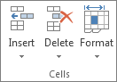
On the Home tab, in the Cells group, click Format.
-
Under Cell Size, do one of the following:
-
To fit all text in the cell, click AutoFit Column Width.
-
To specify a larger column width, click Column Width, and then type the width that you want in the Column width box.
-
Note: As an alternative to increasing the width of a column, you can change the format of that column or even an individual cell. For example, you could change the date format so that a date is displayed as only the month and day («mm/dd» format), such as 12/31, or represent a number in a Scientific (exponential) format, such as 4E+08.
Wrap text in a cell
You can display multiple lines of text inside a cell by wrapping the text. Wrapping text in a cell does not affect other cells.
-
Click the cell in which you want to wrap the text.
-
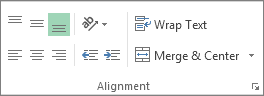
On the Home tab, in the Alignment group, click Wrap Text.
Note: If the text is a long word, the characters won’t wrap (the word won’t be split); instead, you can widen the column or decrease the font size to see all the text. If all the text is not visible after you wrap the text, you might have to adjust the height of the row. On the Home tab, in the Cells group, click Format, and then under Cell Size click AutoFit Row.
For more information on wrapping text, see the article Wrap text in a cell.
Change the format of a number
In Excel, the format of a cell is separate from the data that is stored in the cell. This display difference can have a significant effect when the data is numeric. For example, when a number that you enter is rounded, usually only the displayed number is rounded. Calculations use the actual number that is stored in the cell, not the formatted number that is displayed. Hence, calculations might appear inaccurate because of rounding in one or more cells.
After you type numbers in a cell, you can change the format in which they are displayed.
-
Click the cell that contains the numbers that you want to format.
-
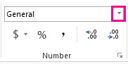
On the Home tab, in the Number group, click the arrow next to the Number Format box, and then click the format that you want.
To select a number format from the list of available formats, click More Number Formats, and then click the format that you want to use in the Category list.
Format a number as text
For numbers that should not be calculated in Excel, such as phone numbers, you can format them as text by applying the Text format to empty cells before typing the numbers.
-
Select an empty cell.
-
On the Home tab, in the Number group, click the arrow next to the Number Format box, and then click Text.
-
Type the numbers that you want in the formatted cell.
Numbers that you entered before you applied the Text format to the cells must be entered again in the formatted cells. To quickly reenter numbers as text, select each cell, press F2, and then press Enter.
Need more help?
You can always ask an expert in the Excel Tech Community or get support in the Answers community.
Need more help?
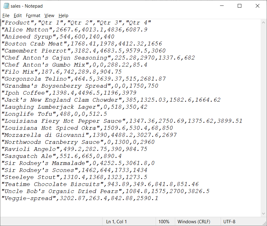
This VBA Program reads an Excel Range (Sales Data) and write to a Text file (Sales.txt)
Excel VBA code to read data from an Excel file (Sales Data – Range “A1:E26”). Need two “For loop” for rows and columns. Write each value with a comma in the text file till the end of columns (write without comma only the last column value). Do the above step until reach the end of rows.
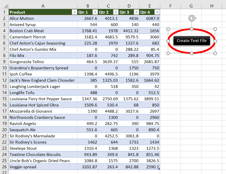
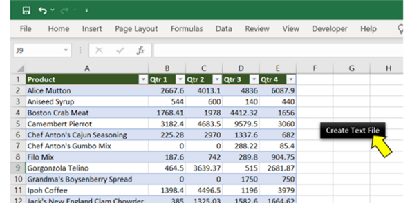
Sales Data in Excel: 5 columns and 25 rows
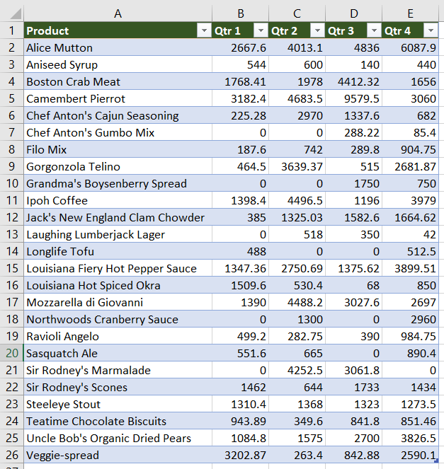
Sales Data
VBA code to create a text file as below
VBA Code:
- Declaring Variables :
| Variable | Data Type | Comments |
|---|---|---|
| myFileName | String | Output text file (Full path with file name) |
| rng | Range | Excel range to read |
| cellVal | Variant | Variable to assign each cell value |
| row | Integer | Iterate rows |
| col | Integer | Iterate columns |
'Variable declarations
Dim myFileName As String, rng As Range, cellVal As Variant, row As Integer, col As Integer
- Initialize variables:
- myFileName: The file name with the full path of the output text file
- rng: Excel range to read data from an excel.
'Full path of the text file
myFileName = "D:ExcelWriteTextsales.txt"
'Data range need to write on text file
Set rng = ActiveSheet.Range("A1:E26")
Open the output text file and assign a variable “#1”
'Open text file
Open myFileName For Output As #1
‘Nested loop to iterate both rows and columns of a given range eg: “A1:E26” [5 columns and 26 rows]
'Number of Rows
For row = 1 To rng.Rows.Count
   'Number of Columns
   For col = 1 To rng.Columns.Count
Assign the value to variable cellVal
cellVal = rng.Cells(row, col).Value
Write cellVal with comma. If the col is equal to the last column of a row. write-only value without the comma.
'write cellVal on text file
    If col = rng.Columns.Count Then
        Write #1, cellVal
    Else
        Write #1, cellVal,
    End If
Close both for loops
   Next col
Next row
Close the file
Close #1
Approach:
Step 1: Add a shape (Create Text File) to your worksheet
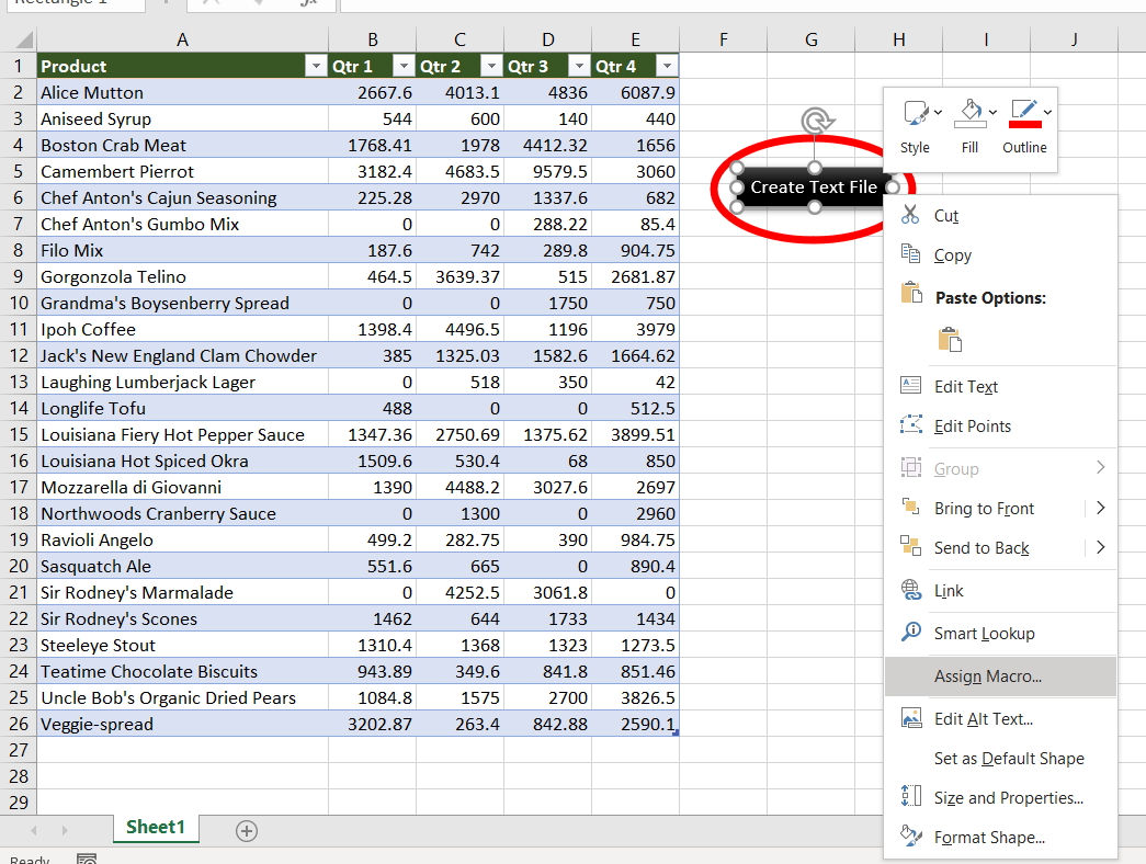
Step 2: Right-click on “Create a Text file” and “Assign Macro..”
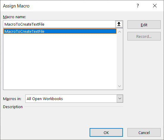
Step 3: Select MacroToCreateTextFile
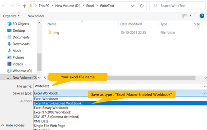
Step 4: Save your excel file as “Excel Macro-Enabled Workbook” *.xlsm
Step 5: Click “Create Text file”
The following sections explain how to write various types of data to an Excel
worksheet using XlsxWriter.
Writing data to a worksheet cell
The worksheet write() method is the most common means of writing
Python data to cells based on its type:
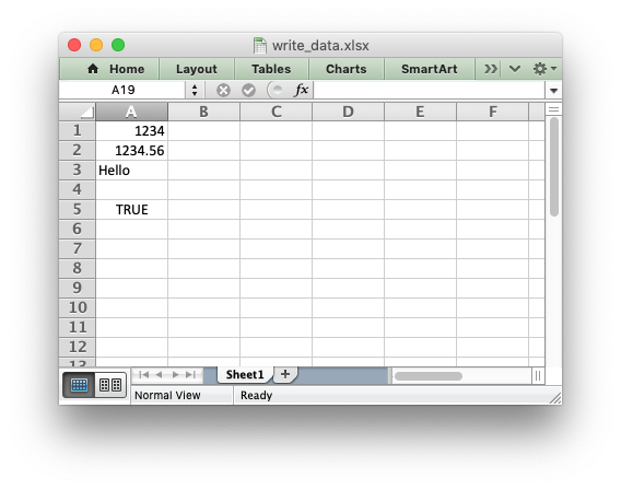
import xlsxwriter

workbook = xlsxwriter.Workbook('write_data.xlsx')
worksheet = workbook.add_worksheet()

worksheet.write(0, 0, 1234)     # Writes an int
worksheet.write(1, 0, 1234.56)  # Writes a float
worksheet.write(2, 0, 'Hello')  # Writes a string
worksheet.write(3, 0, None)     # Writes None
worksheet.write(4, 0, True)     # Writes a bool

workbook.close()
The write() method uses the type() of the data to determine which
specific method to use for writing the data. These methods then map some basic
Python types to corresponding Excel types. The mapping is as follows:
| Python type | Excel type | Worksheet methods |
|---|---|---|
int |
Number | write(), write_number() |
long |
||
float |
||
Decimal |
||
Fraction |
||
basestring |
String | write(), write_string() |
str |
||
unicode |
||
None |
String (blank) | write(), write_blank() |
datetime.date |
Number | write(), write_datetime() |
datetime.datetime |
||
datetime.time |
||
datetime.timedelta |
||
bool |
Boolean | write(), write_boolean() |
The write() method also handles a few other Excel types that are
encoded as Python strings in XlsxWriter:
| Pseudo-type | Excel type | Worksheet methods |
|---|---|---|
| formula string | Formula | write(), write_formula() |
| url string | URL | write(), write_url() |
It should be noted that Excel has a very limited set of types to map to. The
Python types that the write() method can handle can be extended as
explained in the Writing user defined types section below.
Writing lists of data
Writing compound data types such as lists with XlsxWriter is done the same way
it would be in any other Python program: with a loop. The Python
enumerate() function is also very useful in this context:
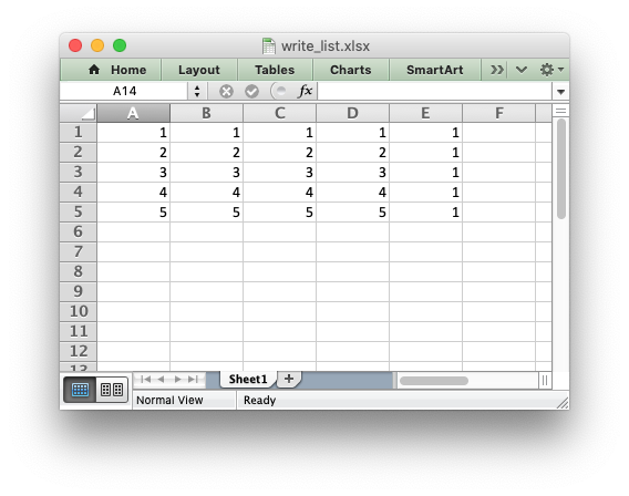
import xlsxwriter

workbook = xlsxwriter.Workbook('write_list.xlsx')
worksheet = workbook.add_worksheet()

my_list = [1, 2, 3, 4, 5]

for row_num, data in enumerate(my_list):
    worksheet.write(row_num, 0, data)

workbook.close()
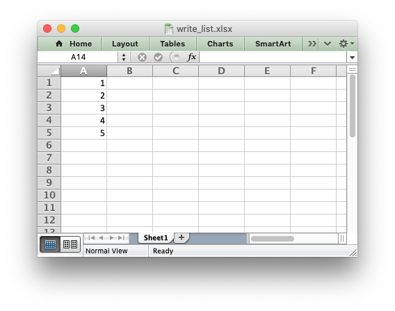
Or if you wanted to write this horizontally as a row:
import xlsxwriter

workbook = xlsxwriter.Workbook('write_list.xlsx')
worksheet = workbook.add_worksheet()

my_list = [1, 2, 3, 4, 5]

for col_num, data in enumerate(my_list):
    worksheet.write(0, col_num, data)

workbook.close()

For a list of lists structure you would use two loop levels:
import xlsxwriter

workbook = xlsxwriter.Workbook('write_list.xlsx')
worksheet = workbook.add_worksheet()

my_list = [[1, 1, 1, 1, 1],
           [2, 2, 2, 2, 1],
           [3, 3, 3, 3, 1],
           [4, 4, 4, 4, 1],
           [5, 5, 5, 5, 1]]

for row_num, row_data in enumerate(my_list):
    for col_num, col_data in enumerate(row_data):
        worksheet.write(row_num, col_num, col_data)

workbook.close()
The worksheet class has two utility functions called
write_row() and write_column() which are basically a loop around
the write() method:
import xlsxwriter

workbook = xlsxwriter.Workbook('write_list.xlsx')
worksheet = workbook.add_worksheet()

my_list = [1, 2, 3, 4, 5]

worksheet.write_row(0, 1, my_list)
worksheet.write_column(1, 0, my_list)

workbook.close()

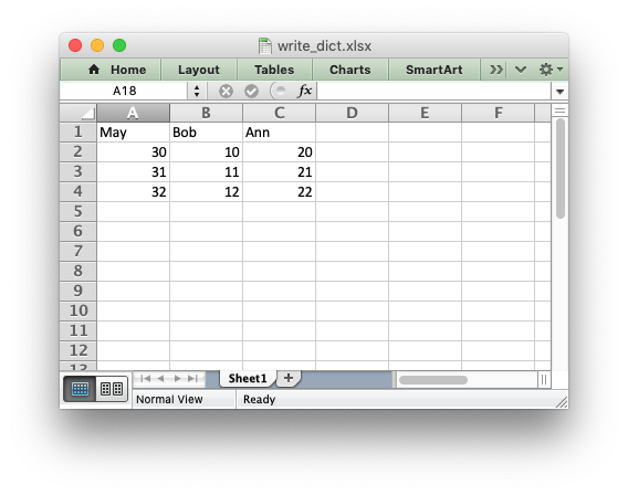
Writing dicts of data
Unlike lists there is no single simple way to write a Python dictionary to an
Excel worksheet using Xlsxwriter. The method will depend of the structure of
the data in the dictionary. Here is a simple example for a simple data
structure:
import xlsxwriter

workbook = xlsxwriter.Workbook('write_dict.xlsx')
worksheet = workbook.add_worksheet()

my_dict = {'Bob': [10, 11, 12],
           'Ann': [20, 21, 22],
           'May': [30, 31, 32]}

col_num = 0
for key, value in my_dict.items():
    worksheet.write(0, col_num, key)
    worksheet.write_column(1, col_num, value)
    col_num += 1

workbook.close()
Writing dataframes
The best way to deal with dataframes or complex data structure is to use
Python Pandas. Pandas is a Python data analysis
library. It can read, filter and re-arrange small and large data sets and
output them in a range of formats including Excel.
To use XlsxWriter with Pandas you specify it as the Excel writer engine:
import pandas as pd

# Create a Pandas dataframe from the data.
df = pd.DataFrame({'Data': [10, 20, 30, 20, 15, 30, 45]})

# Create a Pandas Excel writer using XlsxWriter as the engine.
writer = pd.ExcelWriter('pandas_simple.xlsx', engine='xlsxwriter')

# Convert the dataframe to an XlsxWriter Excel object.
df.to_excel(writer, sheet_name='Sheet1')

# Close the Pandas Excel writer and output the Excel file.
writer.close()
The output from this would look like the following:
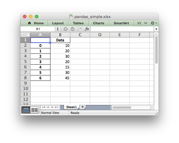
For more information on using Pandas with XlsxWriter see Working with Pandas and XlsxWriter.
Writing user defined types
As shown in the first section above, the worksheet write() method
maps the main Python data types to Excel’s data types. If you want to write an
unsupported type then you can either avoid write() and map the user type
in your code to one of the more specific write methods or you can extend it
using the add_write_handler() method. This can be, occasionally, more
convenient then adding a lot of if/else logic to your code.
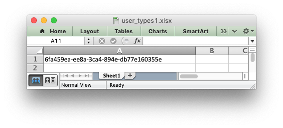
As an example, say you wanted to modify write() to automatically write
uuid types as strings. You would start by creating a function that
takes the uuid, converts it to a string and then writes it using
write_string():
def write_uuid(worksheet, row, col, uuid, format=None):
    return worksheet.write_string(row, col, str(uuid), format)
You could then add a handler that matches the uuid type and calls your
user defined function:
#                           match,     action()
worksheet.add_write_handler(uuid.UUID, write_uuid)
Then you can use write() without further modification:
my_uuid = uuid.uuid3(uuid.NAMESPACE_DNS, 'python.org')

# Write the UUID. This would raise a TypeError without the handler.
worksheet.write('A1', my_uuid)
Multiple callback functions can be added using add_write_handler() but
only one callback action is allowed per type. However, it is valid to use the
same callback function for different types:
worksheet.add_write_handler(int,   test_number_range)
worksheet.add_write_handler(float, test_number_range)
How the write handler feature works
The write() method is mainly a large if() statement that checks the
type() of the input value and calls the appropriate worksheet method to
write the data. The add_write_handler() method works by injecting
additional type checks and associated actions into this if() statement.
Here is a simplified version of the write() method:
def write(self, row, col, *args):

    # The first arg should be the token for all write calls.
    token = args[0]

    # Get the token type.
    token_type = type(token)

    # Check for any user defined type handlers with callback functions.
    if token_type in self.write_handlers:
        write_handler = self.write_handlers[token_type]
        function_return = write_handler(self, row, col, *args)

        # If the return value is None then the callback has returned
        # control to this function and we should continue as
        # normal. Otherwise we return the value to the caller and exit.
        if function_return is None:
            pass
        else:
            return function_return

    # Check for standard Python types, if we haven't returned already.
    if token_type is bool:
        return self.write_boolean(row, col, *args)

    # Etc. ...
The syntax of write handler functions
Functions used in the add_write_handler() method should have the
following method signature/parameters:
def my_function(worksheet, row, col, token, format=None):
    return worksheet.write_string(row, col, token, format)
The function will be passed a worksheet instance, an
integer row and col value, a token that matches the type added to
add_write_handler() and some additional parameters. Usually the
additional parameter(s) will only be a cell format
instance. However, if you need to handle other additional parameters, such as
those passed to write_url() then you can have more generic handling
like this:
def my_function(worksheet, row, col, token, *args):
    return worksheet.write_string(row, col, token, *args)
Note, you don’t have to explicitly handle A1 style cell ranges. These will
be converted to row and column values prior to your function being called.
You can also make use of the row and col parameters to control the
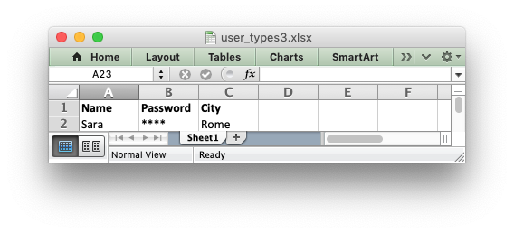
logic of the function. Say for example you wanted to hide/replace user
passwords with ‘****’ when writing string data. If your data was
structured so that the password data was in the second column, apart from the
header row, you could write a handler function like this:
def hide_password(worksheet, row, col, string, format=None):
    if col == 1 and row > 0:
        return worksheet.write_string(row, col, '****', format)
    else:
        return worksheet.write_string(row, col, string, format)
The return value of write handler functions
Functions used in the add_write_handler() method should return one of
the following values:
None: to indicate that control is return to the parentwrite()
method to continue as normal. This is used if your handler function logic
decides that you don’t need to handle the matched token.- The return value of the called
write_xxx()function. This is generally 0
for no error and a negative number for errors. This causes an immediate
return from the callingwrite()method with the return value that was
passed back.
For example, say you wanted to ignore NaN values in your data since Excel
doesn’t support them. You could create a handler function like the following
that matched against floats and which wrote a blank cell if it was a NaN
or else just returned to write() to continue as normal:
def ignore_nan(worksheet, row, col, number, format=None):
    if math.isnan(number):
        return worksheet.write_blank(row, col, None, format)
    else:
        # Return control to the calling write() method.
        return None
If you wanted to just drop the NaN values completely and not add any
formatting to the cell you could just return 0, for no error:
def ignore_nan(worksheet, row, col, number, format=None):
    if math.isnan(number):
        return 0
    else:
        # Return control to the calling write() method.
        return None
This is a submission of the Enhance your bot building with templates blog post series. In this blog post, I will show you how to automate a process on writing data into an excel file.
Steps to follow:
1.Create a project
2.Include the Excel Script Library
3. Add Activities and functions from ‘Excel Lib’ category
4.Set the data that has to be written to the Excel.
5. Save the excel.
Pre-requisites: Desktop Studio :1.0.8.36 MS Office
Instructions:
1. Create a project and a workflow.
Create a new project. Create a new workflow using Workflow perspective.
2. Include the Excel Library for the project.

3. Add the activities from the Excel Lib.
As the first step in the workflow, include the Activity Initialize Excel to initialize Excel Library.
4. Create a new excel file.
Use the activity Create Excel file to create a new excel file. If you want to write data into an existing excel file use the activity Open Existing Excel file. In this blog, I am creating a new excel file.
5. Activate your worksheet to write data into excel.

6. Prepare Excel data
Create an activity Custom to write the below code. Custom activity is used to add manual code. The excel data should be in an array format. Create an item with an array in the Context. Click on the checkbox, to make the item as an array.

Prepare your Excel data in an array format as below.
        rootData.aExcelData[0] = ['Account ID','Opportunity ID','Status'];
	rootData.aExcelData[1] = ['4892737','1223','Open'];
	rootData.aExcelData[2] = ['4358635','987','Closed'];
	rootData.aExcelData[3] = ['68989','8999','In Process'];
6.Set the data into excel.
Use activity Set Values to write the values to the excel. Enter the parameters as below. Excel has a starting column as A and starting row as 1. The data that has to be written to the excel is bound to the field Data.

7. Save the excel
Use the activity Save as Excel to save the new excel file. Enter the location and name of the excel file to be saved.

8.Close the Excel File
Use the activity Close Excel File to close the existing excel file.
9.End Excel file
Use the activity End Excel in order to close the Excel Library once you are done using it in your project
10. Final workflow looks as below

Output
The file is saved in the mentioned location with the output as below.

Conclusion
This blog post should help you to understand the use of the ‘Excel Library’ and how to write data into excel.
Data Table in Excel (Table of Contents)
- Data Table in Excel
- How to Create Data Table in Excel?
Data Table in Excel
Data tables are used to analyze the changes seen in your final result when certain variables are changed from your function or formula. Data tables are one of the existing parts of What-If analysis tools, which allow you to observe your result by experimenting it with different values of variables and to compare the outcomes stored by the data table.
There are two types of a data table, which are as follows:
- One-Variable Data Table.
- Two-Variable Data Table.
How to Create Data Table in Excel?
Data Table in Excel is very simple and easy to create. Let’s understand the working of the Data Table in Excel by Some Examples.
You can download this Data Table Excel Template here – Data Table Excel Template
Data Table in Excel Example #1 – One-Variable Data Table
One-variable data tables are efficient in the case of analyzing the changes in the result of your formula when you change the values for a single input variable.
Use case of One-Variable Data Table in Excel:
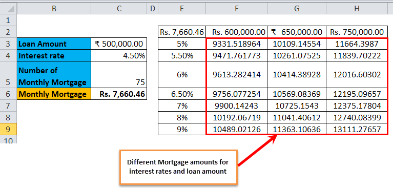
The one-variable data table is useful in scenarios where a person can observe how different interest rates change the amount of their mortgage amount to be paid. Consider the below figure, which shows the mortgage amount calculated based on the interest rate using the PMT function.
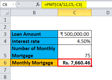
The table above shows the data where the mortgage amount is calculated based on the interest rate, mortgage period and loan amount. It uses the PMT formula to calculate the monthly mortgage amount, which can be written as =PMT (C4/12, C5,-C3).
In the case of observing the monthly mortgage amount for different interest rates, where the interest rate is considered as a variable. In order to do this, there is a need for creating a one-variable data table. The steps to create the one-variable data table are as follows:
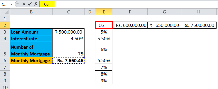
Step 1: Prepare a column which consists of different values for the interest rates. We have entered different values for interest rates in the column which is highlighted in the figure.
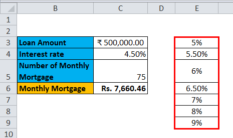
Step 2: In the cell (F2), which is one row above and diagonal to the column which you prepared in the previous step, type this = C6.
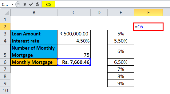
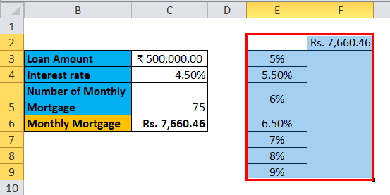
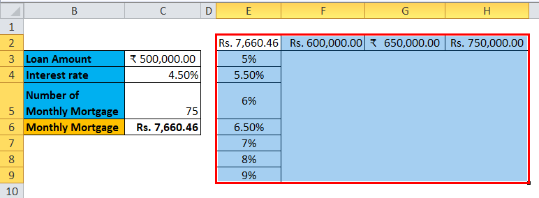
Step 3: Select the entire prepared column by values of different interest rates along with the cell where you had inserted the value, i.e. F2 cell.
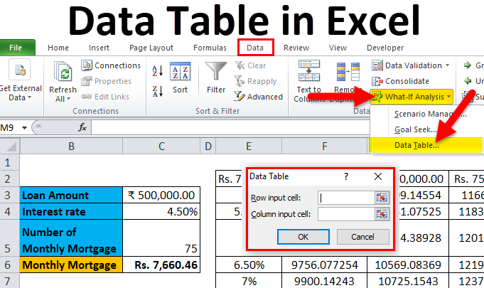
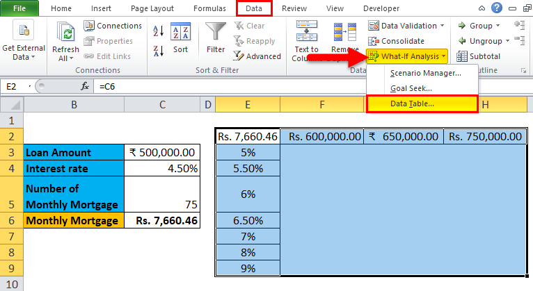
Step 4: Click on the ‘Data’ tab and select ‘What-If Analysis’, and from the options popped down, select ‘Data Table’.
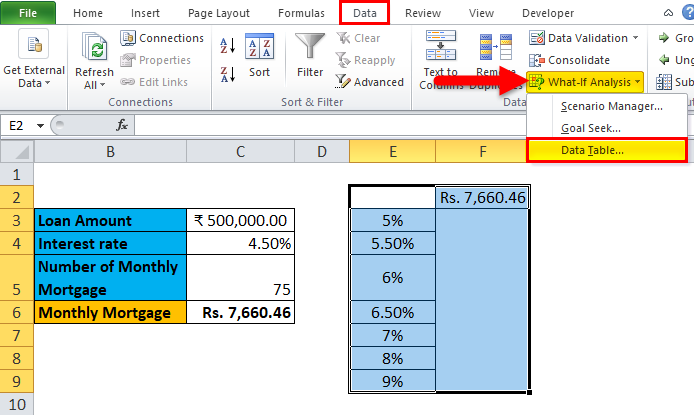
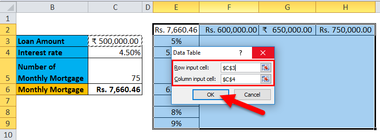
Step 5: Data table dialog box will appear.
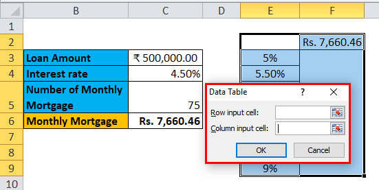
Step 6: In the Column input cell, refer to cell C4 and click OK.
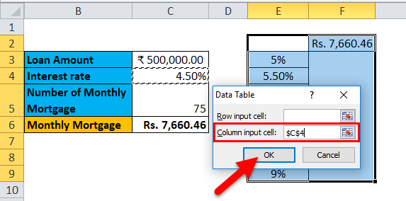
In the dialog box, we refer to the cell C4 in the Column input cell and keep the row input cell empty as we are preparing a data table with one variable.
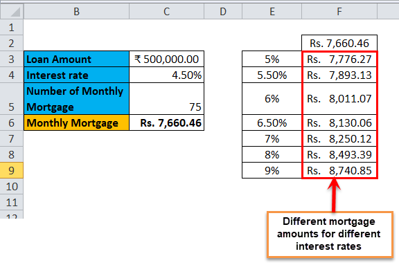
Step 7: After following all the steps, we get all the different mortgage amounts for all entered interests rates in column E (unmarked), and the different mortgage amounts are observed in column F (marked).
Data Table in Excel Example #2 – Two-Variable Data Table
Two-variable data tables are useful in scenarios where a user needs to observe the changes in the result of their formula when they change two input variables simultaneously.
Use-case of Two-Variable Data Table in Excel:
The two-variable data table is useful in scenarios where a person can observe how different interest rates and loan amounts change the amount of their mortgage amount to be paid. Instead of calculating for individual values separately, we can observe them with instantaneous results. Consider the below figure, which shows the mortgage amount calculated based on the interest rate using the PMT function.
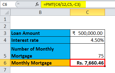
The above example is similar to our example shown in the previous case for a one-variable data table. Here the mortgage amount in cell C6 is calculated based on the interest rate, mortgage period and loan amount. It uses the PMT formula to calculate the monthly mortgage amount, which can be written as =PMT (C4/12, C5,-C3).
In order to explain the two-variable data table with reference to the above example, we will show the different mortgage amounts and choose the best which suits you by observing the different values of interest rates and loan amount. In order to do this, there is a need for creating a two-variable data table. The steps to create the one-variable data table are as follows:
Step 1: Prepare a column which consists of different values for the interest rates and loan amount.
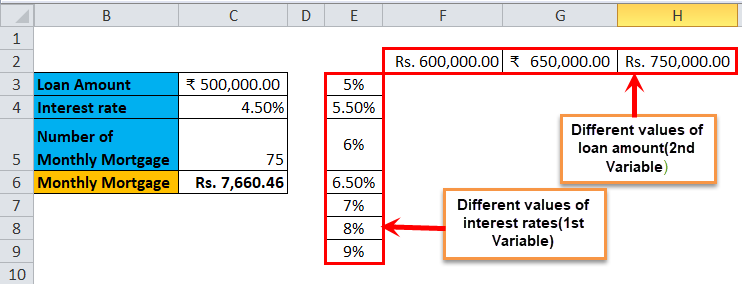
We have prepared a column consisting of the different interest rates, and in the cell diagonal to starting cell of the column, we have entered the different values of the loan amount.
Step 2: In the cell (E2), which is one row above to the column which you prepared in the previous step, type this = C6.
Step 3: Select the entire prepared column by values of different interest rates along with the cell where you had inserted the value, i.e. E2 cell.
Step 4: Click on the ‘Data’ tab and select ‘What-If Analysis’, and from the options popped down, select ‘Data Table’.
Step 5: A Data table dialog box will appear. The ‘Column input cell’ refers to cell C4 and in the ‘Row input cell’ C3. Both the values are selected as we are changing both the variables and Click OK.
Step 6: After following all the steps, we get different values of mortgage amounts for different values of interest rates and loan amount.
Things to Remember About Data Table in Excel
- For one variable data table, the ‘Row input cell’ is left empty, and in a two-variable data table, both ‘Row input cell’ and ‘Column input cell’ are filled.
- Once the What-If analysis is performed, and the values are calculated, you cannot change or modify any cell from the set of values.
Recommended Articles
This has been a guide to a Data Table in Excel. Here we discuss its types and how to create data table examples and downloadable excel templates. You may also look at these useful functions in excel –
- Two-Variable Data Table in Excel
- One Variable Data Table in Excel
- Excel Data Visualization
- Database Function in Excel
Write Data to Worksheet Cell in Excel VBA
Description:
In the previous post we have seen, how to read data from excel to VBA. We will see how to write data to Worksheet Cell in Excel VBA.
Write Data to Worksheet Cell in Excel VBA – Solution(s):
![]() It is same as reading the data from Excel to VBA. We can use Cell or Range Object to write into a Cell.
It is same as reading the data from Excel to VBA. We can use Cell or Range Object to write into a Cell.
Write Data to Worksheet Cell in Excel VBA – An Example of using Cell Object
The following example will show you how to write the data to Worksheet Cell using Cell Object.
Example Codes
In this example I am writing the data to first Cell of the Worksheet.
Sub sbWriteIntoCellData()

Cells(1, 1)="Hello World"
'Here the first value is Row Value and the second one is column value
'Cells(1, 1) means first row first column
End Sub
In this example I am writing the data to first row and fourth column of the worksheet.
Sub sbWriteIntoCellData1()

Cells(1, 4)="Hello World"

End Sub
Write Data to Worksheet Cell in Excel VBA – An Example of using Range Object
The following example will show you how to write the data into Worksheet Cell or Range using Range Object.
Example Codes
In this example I am reading the data from first Cell of the worksheet.
Sub sbRangeData()

Range("A1")="Hello World"
'Here you have to specify the Cell Name which you want to read - A is the Column and 1 is the Row

End Sub
Write Data to Worksheet Cell in Excel VBA – Specifying the Parent Objects
When you are writing the data using Cell or Range object, it will write the data into Active Sheet. If you want to write the data to another sheet, you have to mention the sheet name while writing the data.
The below example is reading the data from Range A5 of Sheet2:
Sub sbRangeData1()

Sheets("Sheet2").Range("A5")="Hello World"
'Here the left side part is sheets to refer and the right side part is the range to read.

End Sub
In the same way you can mention the workbook name, if you are writing the data to different workbooks.
A Powerful & Multi-purpose Templates for project management. Now seamlessly manage your projects, tasks, meetings, presentations, teams, customers, stakeholders and time. This page describes all the amazing new features and options that come with our premium templates.
Save Up to 85% LIMITED TIME OFFER

All-in-One Pack
120+ Project Management Templates
Essential Pack
50+ Project Management Templates
Excel Pack
50+ Excel PM Templates
PowerPoint Pack
50+ Excel PM Templates
MS Word Pack
25+ Word PM Templates
Ultimate Project Management Template
Ultimate Resource Management Template
Project Portfolio Management Templates
Related Posts
-
- Description:
- Write Data to Worksheet Cell in Excel VBA – Solution(s):
- Write Data to Worksheet Cell in Excel VBA – An Example of using Cell Object
- Write Data to Worksheet Cell in Excel VBA – An Example of using Range Object
- Write Data to Worksheet Cell in Excel VBA – Specifying the Parent Objects
VBA Reference
Effortlessly
Manage Your Projects
120+ Project Management Templates
Seamlessly manage your projects with our powerful & multi-purpose templates for project management.
120+ PM Templates Includes:
29 Comments
-
Tamil
February 4, 2015 at 4:42 PM — ReplyHi Madam,
the way of tutor is awesome for Beginners. Thanks a lot
Edward Tamil
-
Waris
March 27, 2015 at 11:09 AM — ReplyHi Team,
I am just starting learning ABC of VBA macro, I hope it is very useful site for such learner like me….
Keep it…
Waris
-
JAVAID IQBAL
June 8, 2015 at 4:39 AM — ReplyHi Madam,
the way of tutor is awesome for Beginners.Thanks a lot
-
JAVAID IQBAL
June 8, 2015 at 4:40 AM — ReplyHi Madam,
Awesome for Beginners.
Thanks a lot
-
PNRao
June 8, 2015 at 9:39 AM — ReplyVery nice feedback! Thanks Javid!
Thanks-PNRao! -
Ekram
July 31, 2015 at 2:20 AM — ReplyI have been trying to learn Macro for sometime. And this is the first site that has been very helpful. I would definitely recommend this site for anyone to understand what to command and how. We need more ppl like you. Thank you for being such a awesome person.
-
Yogesh Kumar
August 30, 2015 at 6:53 PM — ReplyHi,
I am wondering for a VBA code to read entire data from active excel sheet and print line by line in immediate window.
I searched a lot but unfortunately I did not get any code. Can you help me ? Thanks in advance…Yogi
-
PNRao
August 30, 2015 at 11:31 PM — ReplyHi Yogesh,
You can loop through each cell in the used range of a worksheet and print in the immediate window, the below code will check the each cell, and it will print if the value is not blank.Sub sbReadEachCellPrintinImmediateWindow() For Each cell In ActiveSheet.UsedRange.Cells If Trim(cell.Value) <> " Then Debug.Print cell.Value Next End SubHope this helps!
Thanks-PNRao! -
Yogesh Kumar
September 1, 2015 at 12:00 PM — ReplyHi PNRao,
Thanks a lot for your help, this code worked. May I know , how to print excel row data line by line ?
I want to print a row data in one line and next row data should be print in next line in immediate window or Is there any way to print entire excel sheet data in tabular form in immediate window. Please let me know if this is possible. Thank you in advance.Thanks
Yogi -
Yogesh Kumar
September 2, 2015 at 11:56 AM — ReplySub show()
Dim Arr() As Variant
Arr = Range(“A1:I12”)
Dim R As Long
Dim C As Long
For R = 1 To UBound(Arr, 1)
For C = 1 To UBound(Arr, 2)
Debug.Print Arr(R, C)
Next C
Next REnd Sub
This code prints a range as column in immediate window. Can any one tell me how to print data line by line ? I want to print one row data in one line and next data from next row should be print in next line in immediate window. Please help. Thanks in advance.
Yogi
-
PNRao
September 2, 2015 at 11:12 PM — ReplyHi Yogesh,
You need a small change in your code, see the below code to print each row in one line. In this example, we are storing all the data in a variable and printing for each record:Sub show() Dim Arr() As Variant Arr = Range("A1:I12") Dim R As Long Dim C As Long For R = 1 To UBound(Arr, 1) strnewRow = " For C = 1 To UBound(Arr, 2) strnewRow = strnewRow & " " & Arr(R, C) Next C Debug.Print strnewRow Next R End SubThanks-PNRao!
-
Yogesh Kumar
September 3, 2015 at 1:31 PM — ReplyThank you very much PNRao. This code prints data exactly as per my need.
You are genius ! Hats off to you. Thanks a lot for your help. -
PNRao
September 3, 2015 at 3:59 PM — ReplyYou are most welcome Yogesh! I am glad you found this useful.
Thanks-PNRao! -
Yogesh Kumar
September 6, 2015 at 2:30 PM — ReplyHi
Sub show()
Dim Arr() As Variant
Arr = Range(“A1:I12″)
Dim R As Long
Dim C As Long
For R = 1 To UBound(Arr, 1)
strnewRow = ”
For C = 1 To UBound(Arr, 2)
strnewRow = strnewRow & ” ” & Arr(R, C)
Next C
Debug.Print strnewRowNext R
End SubIn this code I have to do some modifications that this code can read only even columns. Please help me.
Thanks in advance. -
driqbal
October 16, 2015 at 11:31 PM — ReplyYogesh Kumar September 6, 2015 at 2:30 PM
Reply
you need very little modification
Sub show()Dim Arr() As Variant
Arr = Range(“A1:I12”)
Dim R As Long
Dim C As Long
For R = 1 To UBound(Arr, 1)
strnewRow = “”
For C = 2 To UBound(Arr, 2) step 2
strnewRow = strnewRow & ” ” & Arr(R, C)
Next C
Debug.Print strnewRowNext R
End SubThis code will read only even columns.
-
driqbal
October 16, 2015 at 11:33 PM — ReplySub show()
Dim Arr() As Variant
Arr = Range(“A1:I12”)
Dim R As Long
Dim C As Long
For R = 1 To UBound(Arr, 1)
strnewRow = “”
For C = 1 To UBound(Arr, 2)
strnewRow = strnewRow & ” ” & Arr(R, C)
Next C
Debug.Print strnewRowNext R
End Sub -
Jon
November 6, 2015 at 3:26 PM — ReplyI am a V basic user of excel but have created a time sheet at work, i would like to take the information from these sheets completed by multiple people and bring the m together on one sheet is this possible, is it reasonably simple?
Any help would be great.
-
PNRao
November 7, 2015 at 11:21 AM — ReplyHi Jon,
We can use VBA to combine the data from different sheets and workbooks. It can be done in couple of hours based on the requirement. Please let us know if you want us to do this for you.Thanks-PNRao!
-
Abhishek
November 9, 2015 at 10:44 AM — ReplyHi,
I need one big help . Basically, i have 3 worksheets wherein one is the main template ,other one is mapping sheet and third one is the actual scattered data . Now i have to create a macro and run the same for multiple sheets with multiple formats. So, how we can write the vba code to read the scattered data from the 3rd worksheet and through mapping worksheet we can have the data entered into the main template . As the header available in in main template for eg . description can be different like description-value in the other worksheet having scattered data . So we have to use the mapping sheet to get the correct value .Kindly help
-
PNRao
November 9, 2015 at 3:39 PM — ReplyHi Abhishek,
We can use VBA to read the scattered data from the defined worksheet. It will take 2-3 hours based on the requirement. Please let us know if you want us to do this for you.Thanks-PNRao!
-
David
January 13, 2016 at 11:45 PM — ReplyI have a set of data A1:L171 that needs to be merged to multiple Excel templates. However, I only need B,F,G,H (Client, Date, Time AM, Time PM). So basically what I am looking for is a mail merge but through Excel. Is this possible?
-
Surendra
March 14, 2016 at 9:23 PM — ReplyI want to create a function which can help me to find if any particular cell has special character or not. can anyone help me out. thanks
-
Desk Tyrant
June 24, 2016 at 11:36 AM — ReplyHey,
thanks for the super quick tutorial. This stuff is pretty complicated at times and it’s hard to find solutions on the internet, but this helped me a bit so thanks again.
-
Claire
July 7, 2016 at 9:35 AM — ReplyHi,
I am trying to change the output from a macro that I have designed which is a series of combo boxes – currently the output is across the sheet, with each combo box selection being input into a consecutive column. I’d like them to be input into consecutive rows (so the text appears in a single column).
The current script that I’m using is:Private Sub CommandButton1_Click()
If Me.ComboBox1.Value = “Select” Then
MsgBox “Please select a wildlife health option”, vbExclamation, “Wildlife Health”
Me.ComboBox1.SetFocus
Exit Sub
End If
If Me.ComboBox2.Value = “Select” Then
MsgBox “Please select an option for normal ecology”, vbExclamation, “Normal ecology”
Me.ComboBox2.SetFocus
Exit Sub
End If
If Me.ComboBox3.Value = “Select” Then
MsgBox “Please select an option for disease”, vbExclamation, “Disease”
Me.ComboBox3.SetFocus
Exit Sub
End IfRowCount = Sheets(“Sheet2”).Range(“A1”).CurrentRegion.Rows.Count
With Sheets(“Sheet2”).Range(“A1”)
.Offset(RowCount, 1).Value = Me.ComboBox1.Value
.Offset(RowCount, 2).Value = Me.ComboBox2.Value
.Offset(RowCount, 3).Value = Me.ComboBox3.Value
End With
End SubAny help appreciated.
Regards,
Claire -
Ratish
September 29, 2016 at 7:27 PM — ReplyHi,
I am new to excel, My requirement is if I click a button on excel it should update the highlighted cell with the name of the person who clicked and with the time stamp
-
Man
October 5, 2016 at 12:41 PM — Reply -
Ram
July 8, 2017 at 3:23 PM — ReplyHi, Can some one help me on below request.
i have created excel sheet with data from columns A to E (inputs: column A,B,C,D and output: E)
how to read output (E column) data if i give input data from column A- D though macros.
-
PNRao
July 17, 2017 at 1:56 PM — ReplyExample:
Range("E1")=Range("A1")+Range("B1")+Range("C1")+Range("D1")
If Range("E1")>70 Then
MsgBox "Good"
Else
MsgBox "Try Again"
End If
Hope this helps!
-
Zach
October 19, 2019 at 12:37 AM — ReplyHello,
Thanks for the cell tip, I was only aware of using Range(“A1”) = “text” to print to excel. Is there a way to print text to excel starting at a specified cell but not stating every other following text cells location.
Effectively Manage Your
Projects and Resources
ANALYSISTABS.COM provides free and premium project management tools, templates and dashboards for effectively managing the projects and analyzing the data.
We’re a crew of professionals expertise in Excel VBA, Business Analysis, Project Management. We’re Sharing our map to Project success with innovative tools, templates, tutorials and tips.
Project Management
Excel VBA
Download Free Excel 2007, 2010, 2013 Add-in for Creating Innovative Dashboards, Tools for Data Mining, Analysis, Visualization. Learn VBA for MS Excel, Word, PowerPoint, Access, Outlook to develop applications for retail, insurance, banking, finance, telecom, healthcare domains.
Page load link
Go to Top


Photo by Mika Baumeister / Unsplash
Excel files are increasingly used to export data from a Web application to share with other applications or just for reporting and business decision-making. In Node.js, you can export data as PDF or CSV, but Excel can also be the preferred output format. We will see how to write data in an Excel file in this post.
If you are interested in how to generate a CSV file with Node.js, check out this article:
Generate a CSV file from data using Node.js
In this post, we will see how to write data coming from a database in a CSV file using Node.js and Typescript. We will a package called csv-writer.
 Teco TutorialsEric Cabrel TIOGO

Set up the project
Make sure you have Node.js installed on your computer before continuing. I prepared a project starter to quickly start a Node.js project with Typescript. Let’s clone it and make it works locally.
git clone https://github.com/tericcabrel/node-ts-starter node-excel-write

cd node-excel-write

yarn install # or npm install

yarn start # or npm run start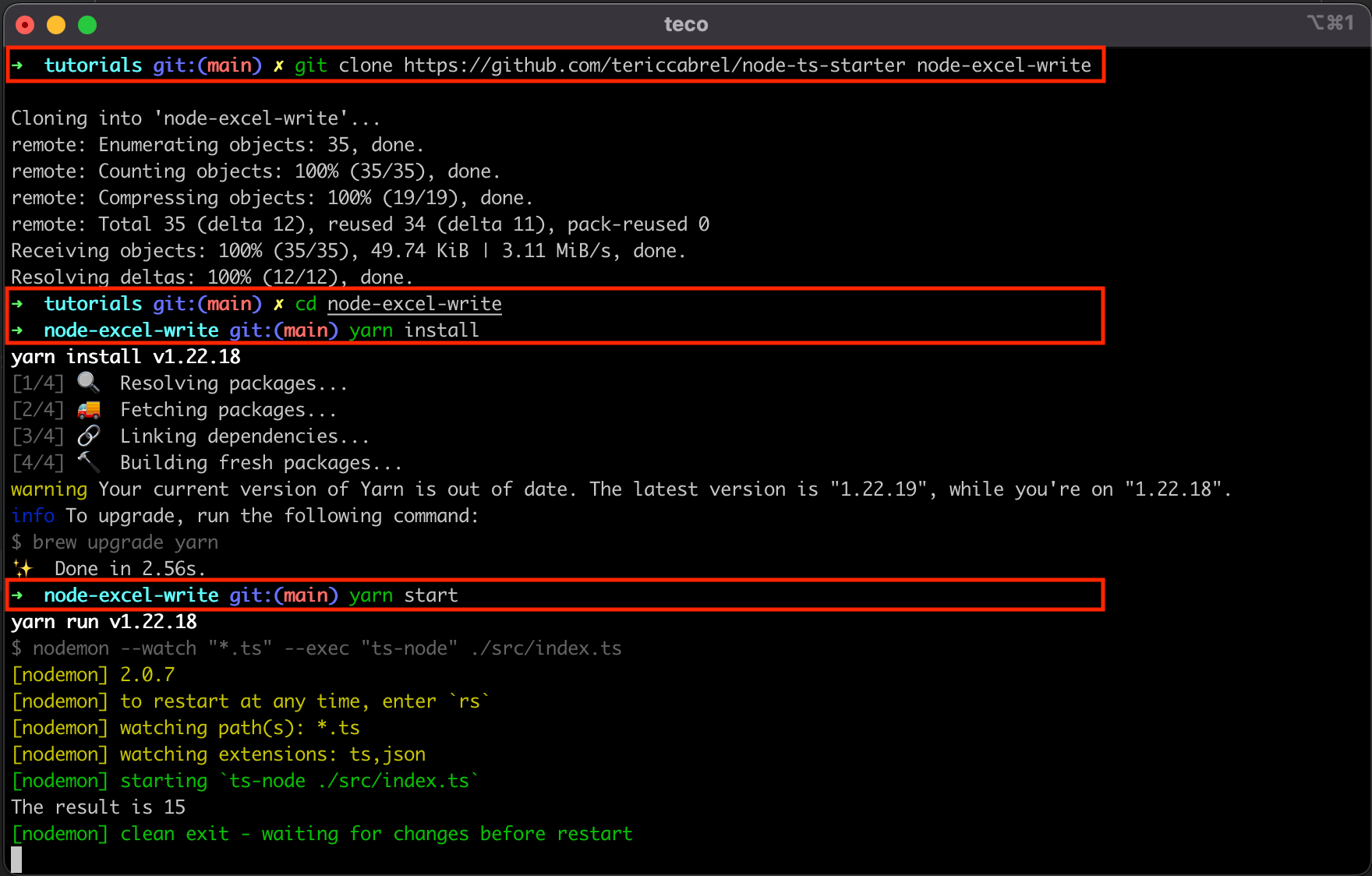
Define the data to write
Let’s say we retrieve a list of countries from the database, and we want to write them in an Excel file. The first is to define the sample of data we want to write.
Replace the content of the file src/index.ts with the code below:
type Country = {
  name: string;
  countryCode: string;
  capital: string;
  phoneIndicator: number;
};

const countries: Country[] = [
  { name: 'Cameroon', capital: 'Yaounde', countryCode: 'CM', phoneIndicator: 237 },
  { name: 'France', capital: 'Paris', countryCode: 'FR', phoneIndicator: 33 },
  { name: 'United States', capital: 'Washington, D.C.', countryCode: 'US', phoneIndicator: 1 },
  { name: 'India', capital: 'New Delhi', countryCode: 'IN', phoneIndicator: 91 },
  { name: 'Brazil', capital: 'Brasília', countryCode: 'BR', phoneIndicator: 55 },
  { name: 'Japan', capital: 'Tokyo', countryCode: 'JP', phoneIndicator: 81 },
  { name: 'Australia', capital: 'Canberra', countryCode: 'AUS', phoneIndicator: 61 },
  { name: 'Nigeria', capital: 'Abuja', countryCode: 'NG', phoneIndicator: 234 },
  { name: 'Germany', capital: 'Berlin', countryCode: 'DE', phoneIndicator: 49 },
];
Note: I get the information about countries here: https://restcountries.com
Install the package ExcelJS
ExcelJS is an excellent library for manipulating an Excel file from Node.js. We will use it in this post, so let’s install it:
npm install exceljsCreate a sheet
With Excel, you can create many sheets where everything sheet contains different kinds of data.
The first to do with ExcelJS is to create the sheet that will hold the countries list. In the file, index.ts add the code below:
import Excel from 'exceljs';

const workbook = new Excel.Workbook();
const worksheet = workbook.addWorksheet('Countries List');
You can use as many sheets as you want; just give a proper variable name for each sheet.
const worksheetCountries = workbook.addWorksheet('Countries List');
const worksheetContinents = workbook.addWorksheet('Continents List');
const worksheetCities = workbook.addWorksheet('Cities List');
For this post, we only need one sheet.
Define the columns’ header
To create the table header, we need to map each column of the header to a property of the Country object.
Update the file src/index.ts, to add the code below:
const countriesColumns = [
  { key: 'name', header: 'Name' },
  { key: 'countryCode', header: 'Country Code' },
  { key: 'capital', header: 'Capital' },
  { key: 'phoneIndicator', header: 'International Direct Dialling' },
];

worksheet.columns = countriesColumns;
The value of the property key must be a key of the object Country (name, countryCode, capital and phoneIndicator).
The property header can be anything, and it will be displayed as the header in the CSV file.
Write the data to the file
It is straightforward to write the file in the sheet.
countries.forEach((country) => {
  worksheet.addRow(country);
});
That’s it.
The remaining part is to generate the Excel file by providing the path to write the file. The code below does that:
import * as path from 'path';

const exportPath = path.resolve(__dirname, 'countries.xlsx');

await workbook.xlsx.writeFile(exportPath);
If you work with Excel and want to level up your skill, I recommend the guide below, containing 36 tutorials covering Excel basics, functions, and advanced formulas.
36 Excel Tutorials To Help You Master Spreadsheets — Digital.com
Excel spreadsheets are essentially databases. Here are 36 Excel tutorials you can use to master Excel and help your career or business grow.
 Digital.comAkshat Biyani

Wrap up
Here is what the index.ts the file looks like this:
import Excel from 'exceljs';
import path from 'path';

type Country = {
  name: string;
  countryCode: string;
  capital: string;
  phoneIndicator: number;
};

const countries: Country[] = [
  { name: 'Cameroon', capital: 'Yaounde', countryCode: 'CM', phoneIndicator: 237 },
  { name: 'France', capital: 'Paris', countryCode: 'FR', phoneIndicator: 33 },
  { name: 'United States', capital: 'Washington, D.C.', countryCode: 'US', phoneIndicator: 1 },
  { name: 'India', capital: 'New Delhi', countryCode: 'IN', phoneIndicator: 91 },
  { name: 'Brazil', capital: 'Brasília', countryCode: 'BR', phoneIndicator: 55 },
  { name: 'Japan', capital: 'Tokyo', countryCode: 'JP', phoneIndicator: 81 },
  { name: 'Australia', capital: 'Canberra', countryCode: 'AUS', phoneIndicator: 61 },
  { name: 'Nigeria', capital: 'Abuja', countryCode: 'NG', phoneIndicator: 234 },
  { name: 'Germany', capital: 'Berlin', countryCode: 'DE', phoneIndicator: 49 },
];

const exportCountriesFile = async () => {
  const workbook = new Excel.Workbook();
  const worksheet = workbook.addWorksheet('Countries List');

  worksheet.columns = [
    { key: 'name', header: 'Name' },
    { key: 'countryCode', header: 'Country Code' },
    { key: 'capital', header: 'Capital' },
    { key: 'phoneIndicator', header: 'International Direct Dialling' },
  ];

  countries.forEach((item) => {
    worksheet.addRow(item);
  });

  const exportPath = path.resolve(__dirname, 'countries.xlsx');

  await workbook.xlsx.writeFile(exportPath);
};

exportCountriesFile();
Execute the file with the command: yarn start.
A file named countries.xlsx will be generated in the same folder containing the file index.ts. Open the file with an Excel file visualizer.
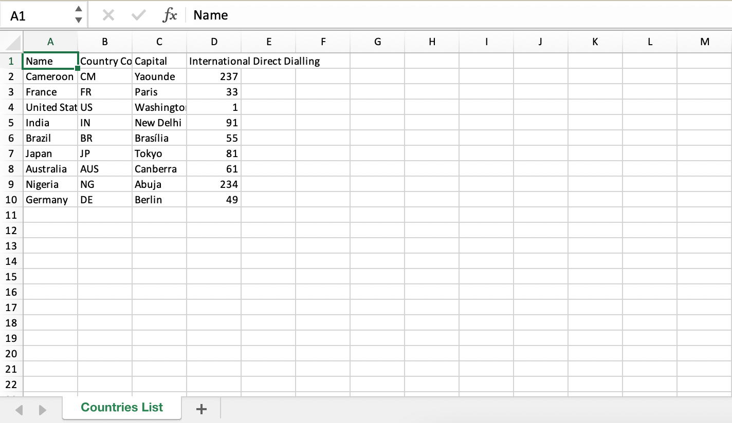
Yeah! it works
Styling the sheet
There is no distinction between the header and other rows on the spreadsheet, and the text’s header overlaps the column width.
We can apply styling on the header to customize the text and increase the column width.
Update the index.ts file with the code below:
worksheet.columns.forEach((sheetColumn) => {
sheetColumn.font = {
size: 12,
};
sheetColumn.width = 30;
});
worksheet.getRow(1).font = {
bold: true,
size: 13,
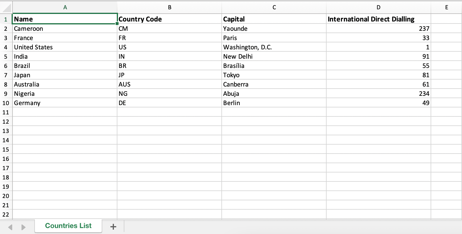
};The forEach() on the worksheet columns will apply the styling, so we first want the font size for all the columns to be 12px and the column width to be 30px.
We want to make the header’s text bold and increase the font size to 13px. We know it is the first line of the sheet. Yeah, the index doesn’t start at 0 but at 1 ?.
Rerun the code to generate a new file, open the generated file again, and tadaaa!
Wrap up
ExcelJS helps you with creating Excel file and writing data inside, but it also allows styling the spreadsheet columns. The support for TypeScript makes the experience of working with great.
Check out the package documentation to learn about other options.
You can find the code source on the GitHub repository.
Follow me on Twitter or subscribe to my newsletter to avoid missing the upcoming posts and the tips and tricks I occasionally share.