
Excel for Microsoft 365 Excel for Microsoft 365 for Mac Excel 2021 Excel 2021 for Mac Excel 2019 Excel 2019 for Mac Excel 2016 Excel 2016 for Mac Excel 2013 Excel 2010 Excel 2007 Excel for Mac 2011 More…Less
By using What-If Analysis tools in Excel, you can use several different sets of values in one or more formulas to explore all the various results.
For example, you can do What-If Analysis to build two budgets that each assumes a certain level of revenue. Or, you can specify a result that you want a formula to produce, and then determine what sets of values will produce that result. Excel provides several different tools to help you perform the type of analysis that fits your needs.
Note that this is just an overview of those tools. There are links to help topics for each one specifically.
What-If Analysis is the process of changing the values in cells to see how those changes will affect the outcome of formulas on the worksheet.
Three kinds of What-If Analysis tools come with Excel: Scenarios, Goal Seek, and Data Tables. Scenarios and Data tables take sets of input values and determine possible results. A Data Table works with only one or two variables, but it can accept many different values for those variables. A Scenario can have multiple variables, but it can only accommodate up to 32 values. Goal Seek works differently from Scenarios and Data Tables in that it takes a result and determines possible input values that produce that result.
In addition to these three tools, you can install add-ins that help you perform What-If Analysis, such as the Solver add-in. The Solver add-in is similar to Goal Seek, but it can accommodate more variables. You can also create forecasts by using the fill handle and various commands that are built into Excel.
For more advanced models, you can use the Analysis ToolPak add-in.
A Scenario is a set of values that Excel saves and can substitute automatically in cells on a worksheet. You can create and save different groups of values on a worksheet and then switch to any of these new scenarios to view different results.
For example, suppose you have two budget scenarios: a worst case and a best case. You can use the Scenario Manager to create both scenarios on the same worksheet, and then switch between them. For each scenario, you specify the cells that change and the values to use for that scenario. When you switch between scenarios, the result cell changes to reflect the different changing cell values.
1. Changing cells
2. Result cell
1. Changing cells
2. Result cell
If several people have specific information in separate workbooks that you want to use in scenarios, you can collect those workbooks and merge their scenarios.
After you have created or gathered all the scenarios that you need, you can create a Scenario Summary Report that incorporates information from those scenarios. A scenario report displays all the scenario information in one table on a new worksheet.
Note: Scenario reports are not automatically recalculated. If you change the values of a scenario, those changes will not show up in an existing summary report. Instead, you must create a new summary report.
If you know the result that you want from a formula, but you’re not sure what input value the formula requires to get that result, you can use the Goal Seek feature. For example, suppose that you need to borrow some money. You know how much money you want, how long a period you want in which to pay off the loan, and how much you can afford to pay each month. You can use Goal Seek to determine what interest rate you must secure in order to meet your loan goal.

Cells B1, B2, and B3 are the values for the loan amount, term length, and interest rate.
Cell B4 displays the result of the formula =PMT(B3/12,B2,B1).
Note: Goal Seek works with only one variable input value. If you want to determine more than one input value, for example, the loan amount and the monthly payment amount for a loan, you should instead use the Solver add-in. For more information about the Solver add-in, see the section Prepare forecasts and advanced business models, and follow the links in the See Also section.
If you have a formula that uses one or two variables, or multiple formulas that all use one common variable, you can use a Data Table to see all the outcomes in one place. Using Data Tables makes it easy to examine a range of possibilities at a glance. Because you focus on only one or two variables, results are easy to read and share in tabular form. If automatic recalculation is enabled for the workbook, the data in Data Tables immediately recalculates; as a result, you always have fresh data.
Cell B3 contains the input value.
Cells C3, C4, and C5 are values Excel substitutes based on the value entered in B3.
A Data Table cannot accommodate more than two variables. If you want to analyze more than two variables, you can use Scenarios. Although it is limited to only one or two variables, a Data Table can use as many different variable values as you want. A Scenario can have a maximum of 32 different values, but you can create as many scenarios as you want.
If you want to prepare forecasts, you can use Excel to automatically generate future values that are based on existing data, or to automatically generate extrapolated values that are based on linear trend or growth trend calculations.
You can fill in a series of values that fit a simple linear trend or an exponential growth trend by using the fill handle or the Series command. To extend complex and nonlinear data, you can use worksheet functions or the regression analysis tool in the Analysis ToolPak Add-in.
Although Goal Seek can accommodate only one variable, you can project backward for more variables by using the Solver add-in. By using Solver, you can find an optimal value for a formula in one cell—called the target cell—on a worksheet.
Solver works with a group of cells that are related to the formula in the target cell. Solver adjusts the values in the changing cells that you specify—called the adjustable cells—to produce the result that you specify from the target cell formula. You can apply constraints to restrict the values that Solver can use in the model, and the constraints can refer to other cells that affect the target cell formula.
Need more help?
You can always ask an expert in the Excel Tech Community or get support in the Answers community.
See Also
Scenarios
Goal Seek
Data Tables
Using Solver for capital budgeting
Using Solver to determine the optimal product mix
Define and solve a problem by using Solver
Analysis ToolPak Add-in
Overview of formulas in Excel
How to avoid broken formulas
Detect errors in formulas
Keyboard shortcuts in Excel
Excel functions (alphabetical)
Excel functions (by category)
Need more help?
Want more options?
Explore subscription benefits, browse training courses, learn how to secure your device, and more.
Communities help you ask and answer questions, give feedback, and hear from experts with rich knowledge.
What is IF Function in Excel?
IF function in Excel evaluates whether a given condition is met and returns a value depending on whether the result is “true” or “false”. It is a conditional function of Excel, which returns the result based on the fulfillment or non-fulfillment of the given criteria.
For example, the IF formula in Excel can be applied as follows:
“=IF(condition A,“value B”,“value C”)”
The IF excel function returns “value B” if condition A is met and returns “value C” if condition A is not met.
It is often used to make logical interpretations which help in decision-making.
Table of contents
- What is IF Function in Excel?
- Syntax of the IF Excel Function
- How to Use IF Function in Excel?
- Example #1
- Example #2
- Example #3
- Example #4
- Example #5
- Guidelines for the Multiple IF Statements
- Frequently Asked Question
- IF Excel Function Video
- Recommended Articles
Syntax of the IF Excel Function
The syntax of the IF function is shown in the following image:

The IF excel function accepts the following arguments:
- Logical_test: It refers to the condition to be evaluated. The condition can be a value or a logical expression.
- Value_if_true: It is the value returned as a result when the condition is “true”.
- Value_if_false: It is the value returned as a result when the condition is “false”.
In the formula, the “logical_test” is a required argument, whereas the “value_if_true” and “value_if_false” are optional arguments.
The IF formula uses logical operators to evaluate the values in a range of cells. The following table shows the different logical operatorsLogical operators in excel are also known as the comparison operators and they are used to compare two or more values, the return output given by these operators are either true or false, we get true value when the conditions match the criteria and false as a result when the conditions do not match the criteria.read more and their meaning.
| Operator | Meaning |
|---|---|
| = | Equal to |
| > | Greater than |
| >= | Greater than or equal to |
| < | Less than |
| <= | Less than or equal to |
| <> | Not equal to |
How to Use IF Function in Excel?
Let us understand the working of the IF function with the help of the following examples in Excel.
You can download this IF Function Excel Template here – IF Function Excel Template
Example #1
If there is no oxygen on a planet, life is impossible. If oxygen is available on a planet, then life is possible. The following table shows a list of planets in column A and the information on the availability of oxygen in column B. We have to find the planets where life is possible, based on the condition of oxygen availability.

Let us apply the IF formula to cell C2 to find out whether life is possible on the planets listed in the table.
The IF formula is stated as follows:
“=IF(B2=“Yes”, “Life is Possible”, “Life is Not Possible”)
The succeeding image shows the IF formula applied to cell C2.

The subsequent image shows how the IF formula is applied to the range of cells C2:C5.

Drag the cells to view the output of all the planets.

The output in the below worksheet shows life is possible on the planet Earth.
Flow Chart of Generic IF Excel Function

The IF Function Flow Chart for Mars (Example #1)

The flow of IF function flowchart for Jupiter and Venus is the same as the IF function flowchart for Mars (Example #1).
The IF Function Flow Chart for Earth

Hence, the IF excel function allows making logical comparisons between values. The modus operandi of the IF function is stated as: If something is true, then do something; otherwise, do something else.
Example #2
The following table shows a list of years. We want to find out if the given year is a leap year or not.
A leap year has 366 days; the extra day is the 29th of February. The criteria for a leap year are stated as follows:
- The year will be exactly divisible by 4 and not exactly be divisible by 100 or
- The year will be exactly divisible by 400.

In this example, we will use the IF function along with the AND, OR, and MOD functions to find the leap years.
We use the MOD function to find a remainder after a dividend is divided by a divisor.
The AND functionThe AND function in Excel is classified as a logical function; it returns TRUE if the specified conditions are met, otherwise it returns FALSE.read more evaluates both the conditions of the leap years for the value “true”. The OR functionThe OR function in Excel is used to test various conditions, allowing you to compare two values or statements in Excel. If at least one of the arguments or conditions evaluates to TRUE, it will return TRUE. Similarly, if all of the arguments or conditions are FALSE, it will return FASLE.read more evaluates either of the condition for the value “true”.
We will apply the MOD function to the conditions as follows:
If MOD(year,4)=0 and MOD(year,100)<>(is not equal to) 0, then the year is a leap year.
or
If MOD(year,400)=0, then the year is a leap year; otherwise, the year is not a leap year.
The IF formula is stated as follows:
“=IF(OR(AND((MOD(year,4)=0),(MOD(year,100)<>0)),(MOD(year,400)=0)),“Leap Year”, “Not A Leap Year”)”
The argument “year” refers to a reference value.
The following images show the output of the IF formula applied in the range of cells.


The following image shows how the IF formula is applied to the range of cells B2:B18.

The succeeding table shows the years 1960, 2028, and 2148 as leap years and the remaining as non-leap years.

The result of the IF excel formula is displayed for the range of cells B2:B18 in the following image.

Example #3
The succeeding table shows a list of drivers and the directions they undertook to reach the destination. It is preceded by an image of the road intersection explaining the turns taken by the drivers and their destinations. The right turn leads to town B, and the left turn leads to town C. Identify the driver’s destination to town B and town C.
Road Intersection Image


Let us apply the IF excel function to find the destination. Here, the condition is mentioned as follows:
- If the driver turns right, he/she reaches town B.
- If the driver turns left, he/she reaches town C.
We use the following IF formula to find the destination:
“=IF(B2=“Left”, “Town C”, “Town B”)”
The succeeding image shows the output of the IF formula applied to cell C2.

Drag the cells to use the formula in the range C2:C11. Finally, we get the destinations of each driver for their turning movements.
The below image displays the IF formula applied to the range.

The output of the IF formula and the destinations are displayed in the succeeding image.

The result shows that six drivers reached town C, and the remaining four have reached town B.
Example #4
The following table shows a list of items and their inventory levels. We want to check if the specific item is available in the inventory or not using the IF function.

Let us list the name of items in column A and the number of items in column B. The list of data to be validated for the entire items list is shown in the cell E2 of the below image.

We use the Excel IF along with the VLOOKUP functionThe VLOOKUP excel function searches for a particular value and returns a corresponding match based on a unique identifier. A unique identifier is uniquely associated with all the records of the database. For instance, employee ID, student roll number, customer contact number, seller email address, etc., are unique identifiers.
read more to check the availability of the items in the inventory.
The VLOOKUP function looks up the values referring to the number of items, and the IF function will check whether the item number is greater than zero or not.
We will apply the following IF formula in the F2 cell:
“=IF(VLOOKUP(E2,A2:B11,2,0)=0, “Item Not Available”,“Item Available”)”
If the lookup value of an item is equal to 0, then the item is not available; else, the item is available.
The succeeding image shows the result of the IF formula in the cell F2.

Select “bat” in the E2 item cell to know whether the item is available or not in the inventory (as shown in the following image).

Example #5
The following table shows the list of students and their marks. The grade criteria are provided based on the marks obtained by the students. We want to find the grade of each student in the list.

We apply the Nested IF in Excel since we have multiple criteria to find and decide each student’s grade.
The Nesting of IF function uses the IF function inside another IF formula when multiple conditions are to be fulfilled.
The syntax of Nesting of IF function is stated as follows:
“=IF( condition1, value_if_true1, IF( condition2, value_if_true2, value_if_false2 ))”
The succeeding table represents the range of scores and the grades, respectively.

Let us apply the multiple IF conditions with AND function in the below-nested formula to find out the grade of the students:
“=IF((B2>=95),“A”,IF(AND(B2>=85,B2<=94),“B”,IF(AND(B2>=75,B2<=84),“C”,IF(AND(B2>=61,B2<=74),“D”,“F”))))”
The IF function checks the logical condition as shown in the formula below:
“=IF(logical_test, [value_if_true],[value_if_false])”
We will split the above-mentioned nested formula and check the IF statements as shown below:
First Logical Test: B2>=95
If the formula returns,
- Value_if_true, execute: “A” (Grade A) else(comma) enter value_if_false
- Value_if_false, then the formula finds another IF condition and enter IF condition
Second Logical Test: B2>=85(logical expression 1) and B2<=94(logical expression 2)
(We use AND function to check the multiple logical expressions as the two given conditions are to be evaluated for “true.”)
If the formula returns,
- Value_if_true, execute: “B” (Grade B) else(comma) enter value_if_false
- Value_if_false, then the formula finds another IF condition and enter IF condition
Third Logical Test: B2>=75(logical expression 1) and B2<=84(logical expression 2)
(We use AND function to check the multiple logical expressions as the two given conditions are to be evaluated for “true.”)
If the formula returns,
- Value_if_true, execute: “C” (Grade C) else(comma) enter value_if_false
- value_if_false, then the formula finds another IF condition and enter IF condition
Fourth Logical Test: B2>=61(logical expression 1) and B2<=74(logical expression 2)
(We use AND function to check the multiple logical expressions as the two given conditions are to be evaluated for “true.”)
If the formula returns,
- Value_if_true, execute: “D” (Grade D) else(comma) enter value_if_false
- Value_if_false, execute: “F” (Grade F)
- Finally, close the parenthesis.
The below image displays the output of the IF formula applied to the range.

The succeeding image shows the IF nested formula applied to the range.

The grades of the students are listed in the following table.

Guidelines for the Multiple IF Statements
The guidelines for the multiple IF statements are listed as follows:
- Use nested IF function to a limited extent as multiple IF statements require a great deal of thought to be accurate.
- Multiple IF statementsIn Excel, multiple IF conditions are IF statements that are contained within another IF statement. They are used to test multiple conditions at the same time and return distinct values. Additional IF statements can be included in the ‘value if true’ and ‘value if false’ arguments of a standard IF formula.read more require multiple parentheses (), which is often difficult to manage. Excel provides a way to check the color of each opening and closing parenthesis to avoid this situation. The last closing parenthesis color will always be black, denoting the end of the formula statement.
- Whenever we pass a string value for the arguments “value_if_true” and “value_if_false” or test a reference against a string value, enclose the string value in double quotes. Passing a string value without quotes will result in “#NAME?” error.
Frequently Asked Question
1. What is the IF function in Excel?
The Excel IF function is a logical function that checks the given criteria and returns one value for a “true” and another value for a “false” result.
The syntax of the IF function is stated as follows:
“=IF(logical_test, [value_if_true], [value_if_false])”
The arguments are as follows:
1. Logical_test – It refers to a value or condition that is tested.
2. Value_if_true – It is the value returned when the condition logical_test is “true.”
3. Value_if_false – It is the value returned when the condition logical_test is “false.”
The “logical_test” is a required argument, whereas the “value_if_true” and “value_if_false” are optional arguments.
2. How to use the IF Excel function with multiple conditions?
The IF Excel statement for multiple conditions is created by using multiple IF functions in a single formula.
The syntax of IF function with multiple conditions is stated as follows:
“=IF (condition 1_“true”, do something, IF (condition 2_“true”, do something, IF (condition 3_ “true”, do something, else do something)))”
3. How to use the function IFERROR in Excel?
IF Excel Function Video
Recommended Articles
This has been a guide to the IF function in Excel. Here we discuss how to use the IF function along with examples and downloadable templates. You may also look at these useful functions –
- What is the Logical Test in Excel?A logical test in Excel results in an analytical output, either true or false. The equals to operator, “=,” is the most commonly used logical test.read more
- “Not Equal to” in Excel“Not Equal to” argument in excel is inserted with the expression <>. The two brackets posing away from each other command excel of the “Not Equal to” argument, and the user then makes excel checks if two values are not equal to each other.read more
- Data Validation ExcelThe data validation in excel helps control the kind of input entered by a user in the worksheet.read more

Excel has its own What-If analysis tools so that you can use worksheet data to create scenarios and see the numerical output based on your scenario setup.
The Goal Seek Tool
Excel’s goal seek tool is the most common What-If analysis tool. When you have a table of data and want to make a change, you use the goal seek tool to make changes to your formulas to see results based on those calculations.
With the membership table, the net revenue of payments is displayed for each day in February. The calculation shows results for each revenue day so that the reviewer can see the actual revenue from each day that subtracts the payment fees. What if the payment fees changed? You might have a payment processor that you’re reviewing that has higher fees or possibly one that has lower fees. How does this change your revenue? You can answer these two scenario questions using a goal seek What-If analysis.
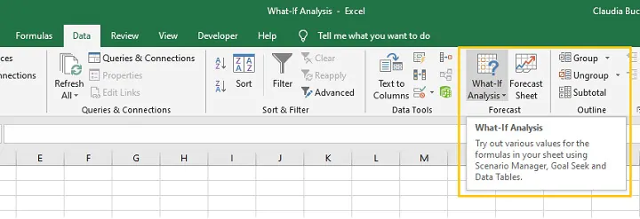
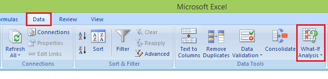
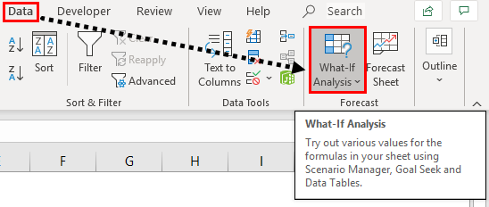
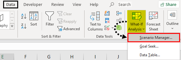
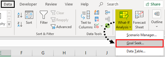
Excel 2019 has three What-If analysis tools. Goal seek is just one of them. The tools to use Excel’s What-If features can be found in Excel’s «Data» menu. Click this menu tab, and then you’ll find the «What-If Analysis» button in the «Forecast» section.
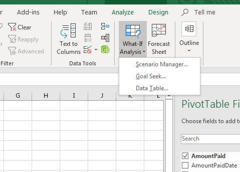
(Whiat-If Analysis button)
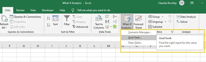
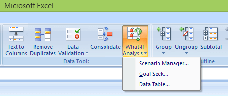
Click the «What-If Analysis» button and a dropdown of options displays. These options are the three different tools that you can use for your What-If analysis. For this example, click the «Goal Seek» option.
(Goal seek configurations)
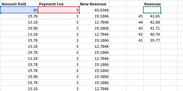
Before you perform a goal seek, you have a few requirements that you must follow before the tool will work. The example uses a pivot table to display data, but goal seek cannot change pivot table data. For this reason, a «Payment Fee» and «New Revenue» columns were created. The payment fee represents the percentage for payments. The new revenue column represents the total amount of revenue by subtracting the payment fee percentage from the gross payment amount.
When working with goal seek tools, the target cell must be a formula. This is because the goal seek tool will take your target value and temporarily change the values in your formula to reach your target scenario.
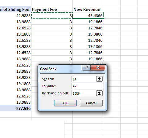
In this example, the scenario identifies the payment fee that you need to use to get to a specific amount. The net revenue currently for the first cell in the «New Revenue» column is 43.4366. This is the cell that contains the formula that calculates how much net revenue is made by subtracting the fee percent from gross revenue. The «Set cell» input text box must contain a cell with a formula, and the E4 column has the formula requirement.
The «To value» input text box is your target amount. You can run several goal seek evaluations on your worksheet data, but you would need to change values and use multiple goal seek scenarios. For this example, the goal 42 is set to see the maximum threshold for a payment fee to keep net revenue at 42 from the original charge amount.
The cell that contains the payment fee that can be altered is D4. The «By changing cell» input text box is the value that you want to alter. For this example, the payment fee is what will change to determine the fee that would result in net revenue of $42.
After you enter your goal seek values, click «OK,» and Excel 2019 changes the values to display results.
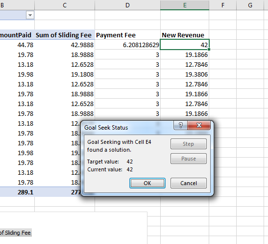
(Goal seek results)
Goal seek searches for a value that would match your scenario results. In this example, the status window displays a notification that it was able to find a value fit suited your requirements. In the spreadsheet, Excel changes the results so that you can see the values that need to change to reach your goals.
In this example, payment fees were increased to examine a threshold for a payment fee that would keep the total net revenue at $42. The result was that payment fees could increase to up to a little over 6% and your total net revenue would not go below $42.
The «Goal Seek Status» window has a «Step» and «Pause» button. With some complex goal seek scenarios, the What-If tool won’t be able to find a value that will match your proposed end result. You can use the «Step» button to add another step to the goal seek or use the «Stop» button to cancel the goal seek procedure and change the values for each input option.
The Scenario Tool
The goal seek tool lets you review one scenario and enter values for one end result. The scenario tool takes this a step further and lets you have multiple values and goals to find variations of your projections. To open a scenario configuration window, click the «Data» tab and then click the «What-If Analysis» button in the «Forecast» section. Clicking the «Scenario Manager» option in the dropdown menu will open a configuration window where you set up your scenarios.

(Scenario Manager window)
Because scenarios let you put together several projections, you have a much more complex configuration window when you work with scenarios. Click «Add» to create your first scenario based on the data in your spreadsheet. This example uses the data from membership charges, payment fees, and net revenue by subtracting fees from gross revenue.
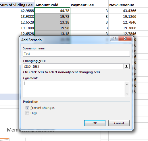
(Add scenario)
Because a scenario lets you review several projects with multiple values, you can enter multiple cells in the «Changing cells» input text box. You can also add cells into this text box by using your mouse and clicking each cell in the worksheet.
Excel 2019 automatically fills in your name with the date the scenario was created in the «Comment» input text box. You can leave this text box blank or add your own comment to organize scenarios when you have several that you want to review. Give your scenario a name by entering a value in the «Scenario name» input text box. When you review a list of scenarios in the future, this name will help you find the one that you’re looking for.
When you are finished configuring your scenario, click «OK» to create it. Now, it’s time to enter the values for the selected cells.
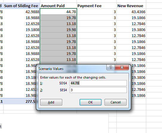
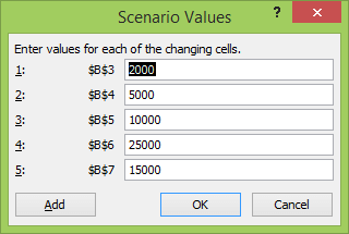
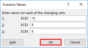
(Scenario values)
The advantage of a scenario over a goal seek is that you can change values in multiple cells, and the next window after creating a scenario is where you configure the values for each cell that you chose to change in the previous window. The default values are the ones that are already entered.
Each cell that you configured in the previous window is displayed with an adjacent input text box where you enter your new values. You can add multiple values, enter just one and leave the others, or any other combination of new values that match your scenario. In this example, the payment fee of 3% is changed to 2% with a total revenue value of $45. Click the «OK» button when you are finished entering new values.
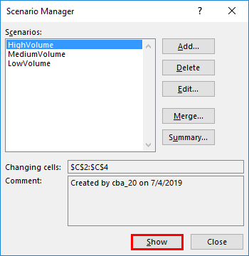
After creating a scenario, you’re returned to a window where you can see a list of all your configured scenarios.
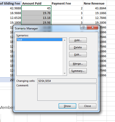
(List of scenarios)
From this window, you can edit, delete or add another scenario. This window is also where you can activate the scenario and view the results of your calculations. Click the scenario that you want to view (in this case «Test) and then click the «Show» button at the bottom of the window.
Clicking «Show» in this example changes the payment fee in the first row to 2 and the total amount paid as 45. The end result is the new revenue value. This value changes to a slightly higher amount. If you want to create another scenario with different values or additional cells to change, you can add another scenario with various changes. With scenarios, you aren’t bound to only one goal with one variable input parameter. You can store multiple scenarios to quickly see the various ways that you can make revenue or manipulate costs so that you make your goals.
When you are finished with your scenario values, click «Close» to exit the window.
Data Tables
With scenarios and the goal seek tools, you set up cells with data that changes based on the variables that you set. For instance, using the payments and fee expenses, you might want to allocate a section of your worksheet that displays a list of possible revenue data points and the net revenue results for a specific payment fee. This example uses a 3% payment fee and then displays several data points with resulting net revenue values.
To create a data table, you first need to set up your column of data.
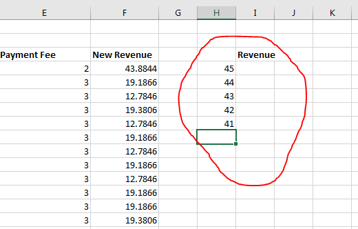
(Data table test data)
In this example, a column of revenue values is set up from $41-$45. To the right of each value is a blank cell with the column header «Revenue.» This column is where the results of your data table calculations will display.
To create the data table, click the «What-If Analysis» button in the «Forecasting» section of the «Data» menu tab. Select «Data Table» from the dropdown menu and a configuration window opens where you can set up your data.
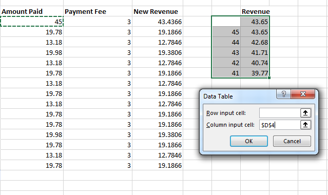
(Data table configuration)
Before you set up the table, you must enter the formula in the first cell under the column label. In this example, the first cell under «Revenue» with the value of 43.65 contains the formula =D4-(D4*E4/100) to calculate the first value in the data table. This formula tells the data table how to calculate the other values.
You must also select the two columns that contain the variable values and the cells to the right of them where the results will display. Make sure you include the cell that has the formula, or the data table will be unable to calculate a result regardless of the number of values you enter.
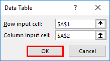
Data tables have two input text boxes that configure them with your selected data. The «Row input cell» text box is where you specify the cell that contains static information for each formula. Since this example will show different net revenue values for a static 3% payment fee, the «Row input cell» text box should be the cell with the payment fee, which is cell E4. However, this data table will use the column row text box.
The «Column input cell» text box contains the original first value 45. The «Row input cell» input text box can be left blank since it won’t be used. Click «OK» and Excel uses the stored formula to configure the values in each row and displays the result in the right adjacent cell. For each column input, the calculation is made and then the results show in the table.
(Data table results)
When you apply the configurations to your data table, the window closes, and you can see the formulated values in the column you chose. With data tables, you can identify values that are used in the calculation because Excel 2019 highlights them in red and blue. This lets you quickly identify which values are used in calculations so that you can understand the information displayed in your worksheet.
Data tables are somewhat different than goal seek and scenario tools, because you can only use static values that are then used to calculate results from a list of input values that you specify in a table. Any alternative formats will fail, and Excel 2019 will give you an error and will not let you complete the data table configuration.
Excel will not let you simply redefine data table data. Once you create it, you must keep it on your worksheet unless you decide to delete it. You can clear a data table by highlighting all column data and pressing the «Delete» key. After you delete the table, you can then redesign and add new configurations to a new table that displays your information.
What-If tools in Excel help you determine the right direction for your finances and business. These tools are beneficial when you have data and want to make a change but you’re unsure of how those changes could result in your financial projections. Excel’s What-If tools are powerful features that can be useful when you want to know what could happen when data changes in your information.
If you’ve ever experimented with different variables to see how your changes would affect the outcome of a situation, you’ve done a what if analysis.
Would you be able to sell more items if you had a sale this week? Or would you make more money by increasing the price instead? In the above scenarios, you want to know the degree to which each change affects the overall outcome. For this reason, a what if analysis is also known as a sensitivity analysis.
Most what if analyses are really mathematical calculations, and that is Excel’s specialty. To help you do a what if analysis, Excel uses commands from the Forecast command group on the Data tab to prepare simple forecasts or advanced business models.
Download your free Excel practice file
Use this free Excel file to practice what if analysis along with the tutorial.
Goal Seek
The simplest sensitivity analysis tool in Excel is Goal Seek. Assuming that you know the single outcome you would like to achieve, the Goal Seek feature in Excel allows you to arrive at that goal by mathematically adjusting a single variable within the equation.
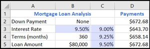
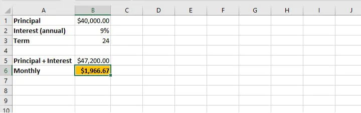
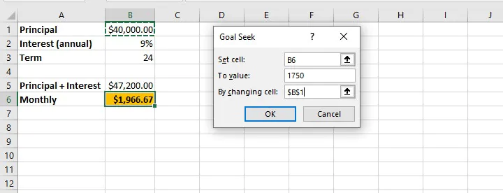
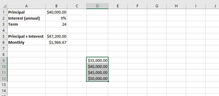
 To illustrate how it works, imagine that the bank is offering an interest rate of 9% per annum on personal loans with 24 months to repay, and that you would like to borrow $40,000.
Using the above information, the bank calculates that the amount borrowed plus interest over the loan period will be $47,200, as shown in cell B5. The amount to be paid each month is also calculated and shown in cell B6.
 By using the Goal Seek command, we can indicate a desired outcome and Excel will determine the adjustment we need to make to a single variable.
In the example above, cell B5 is dependent on the variables in cells B1, B2, and B3. Cell B6 is dependent on cells B3 and B5. Therefore, if we determine that the monthly repayment amount quoted is higher than desired, we can use Goal Seek to set the monthly amount to $1750. Excel can work backwards to change either cell B1, B2, or B3 to reach that goal.
Practically speaking, we may not have much control over the interest rate, so it is more likely that we have the option of adjusting the amount we borrow, or the repayment period.
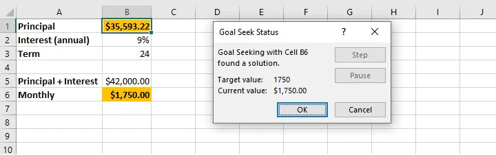
Our first inclination may be to find out how much we will be able to borrow if we pay $1750 per month and all other variables remain the same. Excel will change the principal (B1) based on the number we enter as the new value for cell B6.
 Assuming that the interest amount (9%) and loan period (24 months) remain the same, the new principal amount is calculated and displayed in cell B1 if a valid solution exists.
 Points to note:
- The cell chosen in the “Set cell” field must be a cell containing a formula.
- The cell chosen in the “By changing cell” field must be a cell containing a constant.
- Once “OK” is selected from the Goal Seek Status window, the values on the worksheet are adjusted and are only retrievable by selecting the ‘Undo’ command (Ctrl+Z Windows shortcut/Cmd+Z Mac shortcut).
Scenario Manager
Another what if analysis tool is the Scenario Manager. This option is somewhat more advanced than Goal Seek in that it allows the adjustment of multiple variables at the same time.
 Some other noticeable differences between Goal Seek and Scenario Manager are listed below:
- The Scenario Manager allows the creation of an unlimited number of possible scenarios by changing up to 32 variables at a time.
- Each scenario can be saved for comparative purposes.
- Scenarios may be named and edited, and a brief description provided.
- Only constant values should be changed within the Scenario Manager — cells with formulas should not be manually adjusted.
If we continue our bank loan example, we can determine our model’s sensitivity to change by adjusting any or all of the values in cell B1, B2, or B3.
Best practice
As a best practice, the original worksheet data should be saved as a scenario so that you can revert to it after all the experiments have been completed.
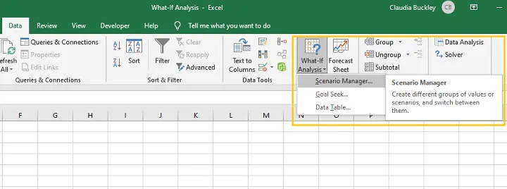
Step 1 — Click ‘What If Analysis’ from the Data tab and select Scenario Manager.
Step 2 — Click ‘Add’ from the Scenario Manager pop-up window.
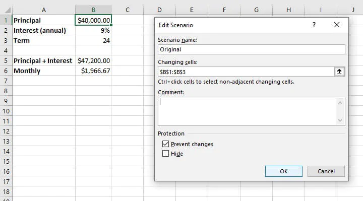
Step 3 — Name this scenario “Original” and enter the cell references of all cells with constant values that you may consider changing in other scenarios (maximum 32 cells). Click OK.
 Step 4 — For the “Original” scenario, do not adjust any values in the ‘Scenario Values’ window.
 Step 5 — Click ‘Add’ to create your first experimental scenario.
Creating experimental scenarios
When creating an experimental scenario, give the scenario a descriptive name from the ‘Add Scenario’ pop-up window. The changing cells will be the same as the ones referenced in your ‘Original’ scenario.
Even if you will not be adjusting all the values in those cells, it is highly recommended that they remain referenced in the ‘changing cells’ field. You may place additional details about the experimental scenario in the ‘Comment’ field (see below).
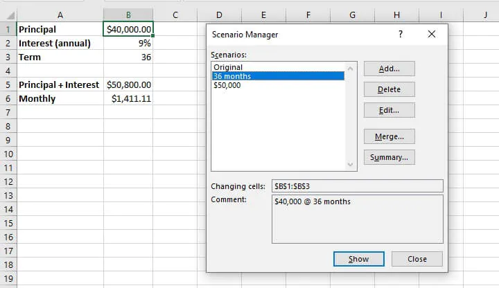
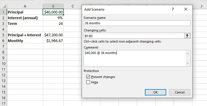 As illustrated above, our experimental scenario is given the name “36 months” and refers to cells B1 to B3 as changing cells. An additional comment indicates that this scenario is to determine the effect of borrowing $40,000 over a 36-month period.
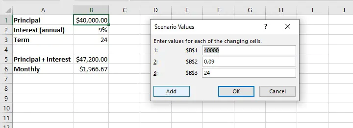
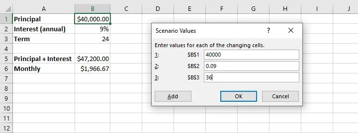
In the ‘Scenario Values’ window, each changing cell is displayed as a field where we can manipulate the constant value so as to affect the outcome of the dependent cells — in our case, cells B5 and B6. As described in our scenario name and comments, we only adjust cell B3 by changing the value to 36.
To add another scenario at this point, select ‘Add’. If not, click OK.
Adjust multiple variables
To experiment with adjusting multiple variables within one scenario, the steps are the same as above, with the exception that the desired changes would be made in the Scenario Values window.
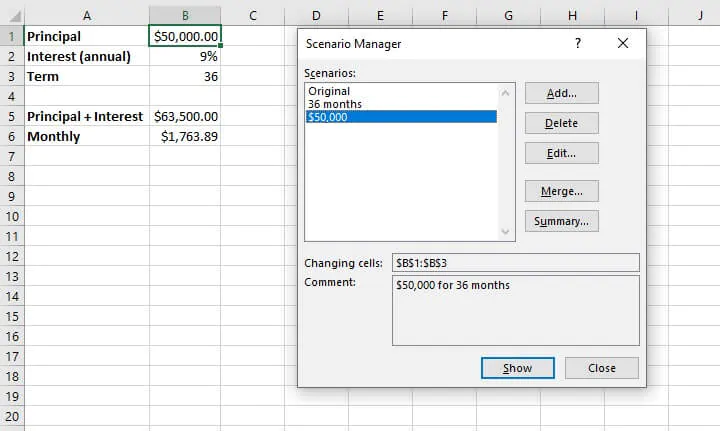
For example, to get Excel to perform a what if analysis on borrowing $50,000 over a 36-month period in the above situation at the same rate of interest, we would simply adjust the fields referencing those variables after creating a new scenario. Excel’s Scenario Manager can handle an unlimited number of scenarios created in this same way.
A list of created scenarios can be viewed by clicking OK from the Scenario Values window, or by selecting Scenario Manager from the What If Analysis dropdown menu.
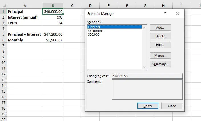 To see the outcome of each adjustment on the output cell(s), either double click on a scenario name, or highlight a name and click Show.
Scenario summary
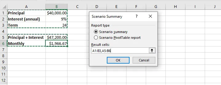
Scenarios that have been created may also be compared side by side with the creation of a Scenario summary worksheet, which is generated by selecting ‘Summary’ from the Scenario Manager window.
There are two report types available — Scenario summary and Scenario PivotTable report. Result cells are the cells that will be displayed in the summary. Ideally, these should include all cells which were adjusted as well as result cells. It’s also a good idea to select cells that contain header names so that these are clearly displayed in the summary.
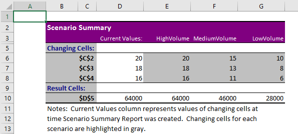
 Choosing the ‘Scenario summary’ option will create a new sheet within the workbook that displays each scenario in columnar format. Changing Cells are highlighted in gray, and Result Cells are displayed under Changing Cells.
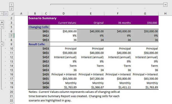 Note that if named ranges were created for Changing or Result Cells, range names will be displayed instead of cell references.
Selecting the Scenario PivotTable report type will create a pivot table report in a new worksheet. Learn more about pivot tables from our Resource Library.
Using data tables for what if analysis
The third what if analysis tool from the Forecast command group is the Data Table. Data tables allow the adjustment of only one or two variables within a dataset, but each variable can have an unlimited number of possible values. Data tables are designed for side-by-side comparisons in a way that makes them easier to read than scenarios, once they are set up correctly.
Data tables are under-utilized, but are not as scary as they may seem.
One-variable data tables
If the only variable to be considered in our loan example were the amount being borrowed, we could set up a one-variable data table.
Step 1 — make a list of all possible principal loan amounts. The list may be by column or row. In our example, we will enter a column list in the range D9 to D12.
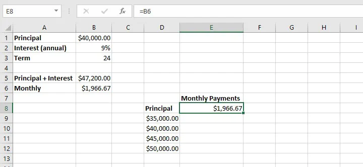
 Step 2 — In an adjacent column, enter the formula which was used to arrive at the original outcome. In this case, we can simply type =B6 in cell E8. This links our new data table to the original variables.
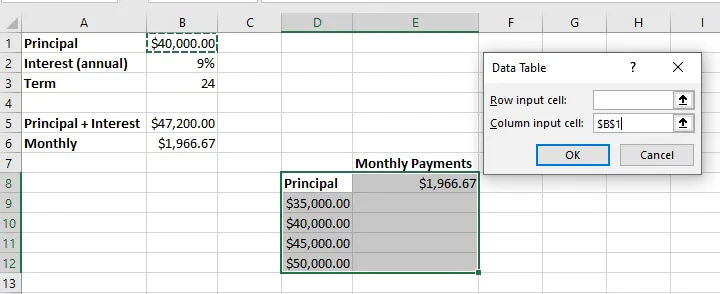
 Step 3 — Select the entire data table range, including the list of variable values, the formula, and blank cells.
Step 4 — From the What If Analysis dropdown menu, select Data Table.
Step 5 — In the column input cell field (since we entered our variables in column format), enter the cell reference that was used to calculate the result in the original dataset. In the above example, this would be cell B1 since this is the variable we have adjusted. No value is entered in the ‘Row input cell’ field in this instance since this is a one-variable data table.
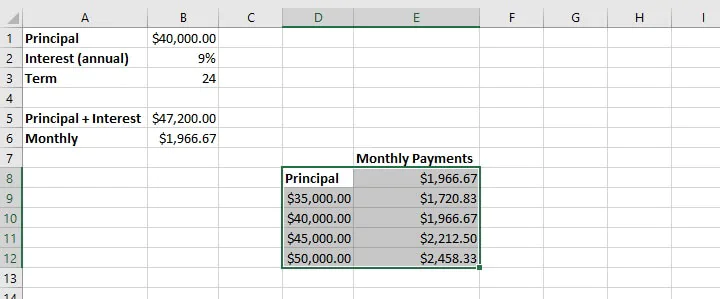
 Step 6 — Select OK. The result is a list of outcomes created by adjusting the one variable in cell B1, assuming that all other variables remain constant.
 To create a row-oriented data table, the variables would be listed horizontally, and the row input cell would be used in the Data Table window instead of the column input cell.
Two-variable data tables
When creating a two-variable data table, one set of values is listed horizontally and the other set is listed vertically. In our example, we will add the loan period (term) as our second variable, displayed horizontally.
In this case, the formula which was used to arrive at the original outcome must be replicated above the vertical list of variables. As shown below, we type =B6 in cell D7. This links our new data table to the original variables.
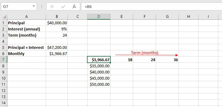 As before, highlight the entire data table range and select Data Table from the What If Analysis menu. The row input cell is the cell reference (B3) that corresponds to the horizontal variables from the original dataset, while the column input cell (B1) corresponds to the vertical variables.
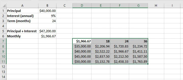
When we select OK, Excel returns a matrix that can be used to compare the outcome of different changes to our original scenario. It may be necessary to adjust the output cells to the appropriate number format for your data type (in the case of the above example, currency).
Summary
Now that you’ve taken the time to demystify how to do a what if analysis in Excel by using these three main tools, why not experiment with using them in different settings — like budget management, profit margin percentages, project completion targets, and the like?
Once you get the hang of these, you’ll want to check out our resource center and take our Basic and Advanced Excel course to become a real pro!
Ready to become a certified Excel ninja?
Start learning for free with GoSkills courses
Start free trial
In Excel, What-if analysis is a process of changing cells’ values to see how those changes will affect the worksheet’s outcome. You can use several different sets of values to explore all the different results in one or more formulas.
What-if Excel is used by almost every data analyst and especially middle to higher management professionals to make better, faster and more accurate decisions based on data. What-if analysis is useful in many situations, such as:
- You can propose different budgets based on revenue.
- You can predict the future values based on the given historical values.
- If you expect a certain value due to a formula, you can find different sets of input values that produce the desired result.
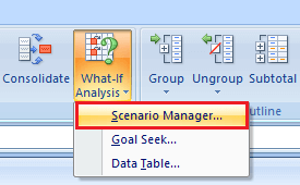
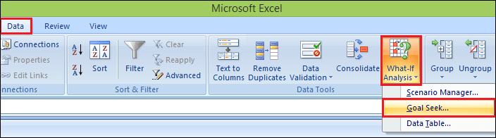
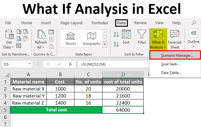
To enable the what-if analysis tool go to the Data menu tab and click on the What-If Analysis option under the Forecast section.
Now click on the What-If Analysis. Excel has the following What-if analysis tools that can be used based on the data analysis needs:
- Scenario Manager
- Goal Seek
- Data Tables
Data Tables and Scenarios take sets of input values and project forward to determine possible results. Goal seek differs from Data Tables and Scenarios in that it takes a result and projects backward to determine possible input values that produce that result.
1. Scenario Manager
A scenario is a set of values that Excel saves and can substitute automatically in cells on a worksheet. Below are the following key features, such as:
- You can create and save different groups of values on a worksheet and then switch to any of these new scenarios to view different results.
- A scenario can have multiple variables, but it can accommodate only up to 32 values.
- You can also create a scenario summary report, which combines all the scenarios on one worksheet. For example, you can create several different budget scenarios that compare various possible income levels and expenses, and then create a report that lets you compare the scenarios side-by-side.
- Scenario Manager is a dialog box that allows you to save the values as a scenario and name the scenario.
2. Goal Seek
Goal Seek is useful if you want to know the formula’s result but unsure what input value the formula needs to get that result. For example, if you want to borrow a loan and know the loan amount, tenure of loan and the EMI that you can pay, you can use Goal Seek to find the interest rate at which you can avail of the loan.
Goal Seek can be used only with one variable input value. If you have more than one variable for input values, you can use the Solver add-in.
3. Data Table
A Data Table is a range of cells where you can change values in some of the cells and answer different answers to a problem. For example, you might want to know how much loan you can afford for a home by analyzing different loan amounts and interest rates. You can put these different values and the PMT function in a Data Table and get the desired result.
A Data Table works only with one or two variables, but it can accept many different values for those variables.
What-If Analysis Scenario Manager
Scenario Manager is one of the What-if Analysis tools in Excel. Scenario Manager is useful in a case where you have more than two variables in the sensitivity analysis. Scenario Manager creates scenarios for each set of the input values for the variables under consideration. Scenarios help you to explore a set of possible outcomes, supporting the following:
- Varying as many as 32 input sets.
- Merging the scenarios from several different worksheets or workbooks.
If you want to analyze more than 32 input sets, and the values represent only one or two variables, you can use Data Tables.
Initial Values for Scenarios
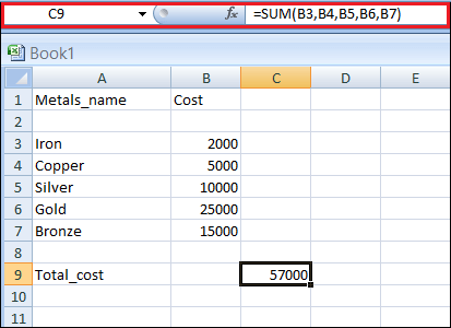
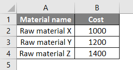
Before you create several different scenarios, you need to define a set of initial values on which the scenarios will be based. Consider an example of a company that wants to buy Metals for their needs. Due to the scarcity of funds, the company wants to understand how much cost will happen for different buying possibilities.
In these cases, we can use the scenario manager for applying different scenarios to understand the results and make the decision accordingly. Now below are the following steps for setting up the initial values for Scenarios:
Step 1: Define the cells that contain the input values.
Step 2: Name the cells Metals_name and Cost.
Step 3: Define the cells that contain the results.
Step 4: Name the result cell Total_cost.
Step 5: place the formula in the result cell.
Step 6: Below is the created table.
To create an analysis report with Scenario Manager, follow the following steps, such as:
Step 1: Click the Data tab.
Step2: Go to the What-If Analysis button and click on the Scenario Manager from the dropdown list.
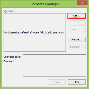
Step 3: Now a scenario manager dialog box appears, click on the Add button to create a scenario.
Step 4: Create the scenario, name the scenario, enter the value for each changing input cell for that scenario, and then click the Ok button.
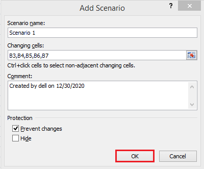
Step 5: Now, B3, B4, B5, B6, and B7 appear in the cells box.
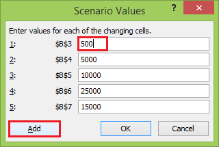
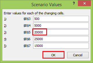
Step 6: Now, change the value of B3to 500 and click the Add button.
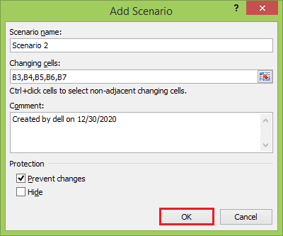
Step 7: After clicking on the Add button, the add scenario dialog box appears again.
- In the scenario name box, create scenario 2.
- Select the prevent changes.
- And click on the Ok
Step 8: Again appears scenario values box with the changed value of B3 cell.
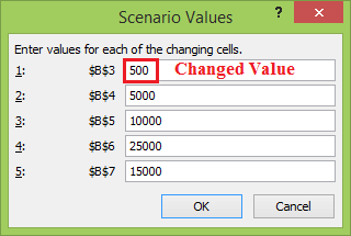
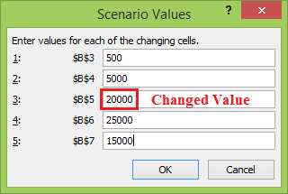
Step 9: Change the value of B5 to 20000 and click the Ok button.
Step 10: Similarly, create Scenario 3 and click the Ok button.

Step 11: Again, appears scenario values box with a changed value of the B5 cell.
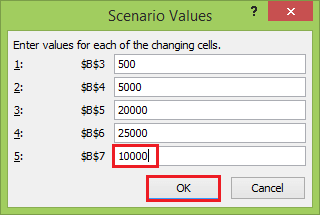
Step 12: Change the value of B7 to 10000 and click the Ok button.
The Scenario Manager Dialog box appears. In the box under Scenarios, You will find the names of all the scenarios that you have created.
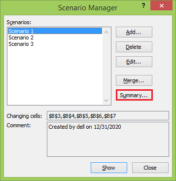
Step 13: Now, click on the Summary button. The Scenario Summary dialog box appears.
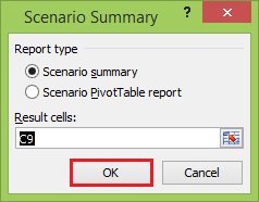
Excel provides two types of Scenario Summary reports:
- Scenario summary.
- Scenario PivotTable report.
Step 14: Select Scenario summary under Report type and click Ok. Scenario Summary report appears in a new worksheet. You will get the following Scenario summary report.
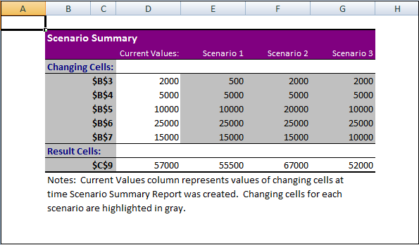
You can observe the following in the Scenario Summary report:
- Changing Cells: Enlists all the cells used as changing cells.
- Result Cells: Displays the result cell specified.
- Current Values: It is the first column and enlists the values of that scenario selected in the Scenario Manager Dialog box before creating the summary report.
- For all the scenarios you have created, the changing cells will be highlighted in gray.
- In the $C$9 row, the result values for each scenario will be displayed.
What-If Analysis Goal Seek
Goal Seek is a What-If Analysis tool that helps you to find the input value that results in a target value that you want. Goal Seek requires a formula that uses the input value to give the result in the target value. Then, by varying the formula’s input value, Goal Seek tries to solve the input value.
Goal Seek works only with one variable input value. If you have more than one input value to be determined, you have to use the Solver add-in. Below are the following steps to use the Goal Seek feature in Excel.
Step 1: On the Data tab, go What-If Analysis and click on the Goal Seek option.
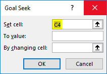
Step 2: The Goal Seek dialog box appears.
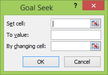
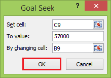
Step 3: Type C9 in the Set cell box. This box is the reference for the cell that contains the formula that you want to resolve.
Step 4: Type 57000 in the To value box. Here, you get the formula result.
Step 5: Type B9 in the By changing cell box. This box has the reference of the cell that contains the value you want to adjust.
Step 6: This cell that the formula must reference goal Seek changes in the cell that you specified in the Set cell box. Click Ok.
Step 7: Goal Seek box produces the following result.
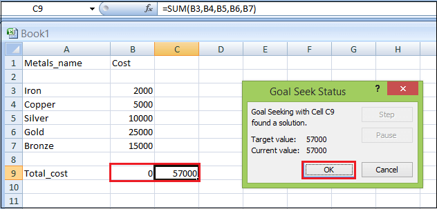
As you can observe, Goal Seek found the solution using B9, and it returns 0 in the B9 cell because the target value and current value are the same.
What-If Analysis Data Tables
With a Data Table in Excel, you can easily vary one or two inputs and perform a What-if analysis. A Data Table is a range of cells where you can change values in some of the cells and answer different answers to a problem. There are two types of Data Tables, such as:
- One-variable data tables
- Two-variable data tables
If you have more than two variables in your analysis problem, you need to use the Excel Scenario Manager Tool.
One-variable Data Tables
A one-variable Data Table can be used to see how different values of one variable in one or more formulas will change those formulas’ results. In other words, with a one-variable Data Table, you can determine how changing one input changes any number of outputs. Below is an example of creating a one-variable data table.
A good example of a data table employs the PMT function with different loan amounts and interest rates to calculate the loan.
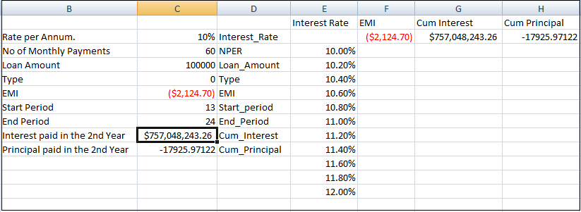
There is a loan of 1 00,000 for a tenure of 5 years. You want to know the monthly payments (EMI) for varied interest rates. You also want to know the amount of interest and Principal that is paid in the second year.
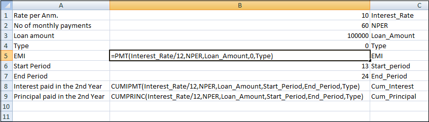
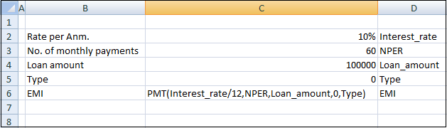
Step 1: Create the required table.
- Assume that the interest rate is 10%.
- List all the required values.
- Name the cells containing the values.
- Set the calculation for EMI, Cumulative Interest and Cumulative Principal with the Excel functions PMT, CUMIPMT and CUMPRINC, respectively.
- Below is the created table.
Step 2: Type the list of interest rate values that you want to substitute in the input cell.
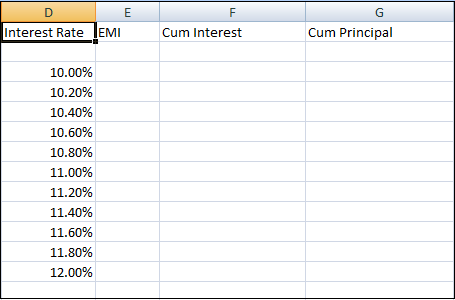
As you observe, there is an empty row above the Interest Rate values. This row is for the formulas.
Step 3: Type the first function (PMT) in the cell one row above and one cell to the right of the column of values. Type the other functions (CUMIPMT and CUMPRINC) in the cells to the first function’s right.
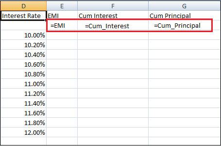
Step 4: The Data Table looks as given below.
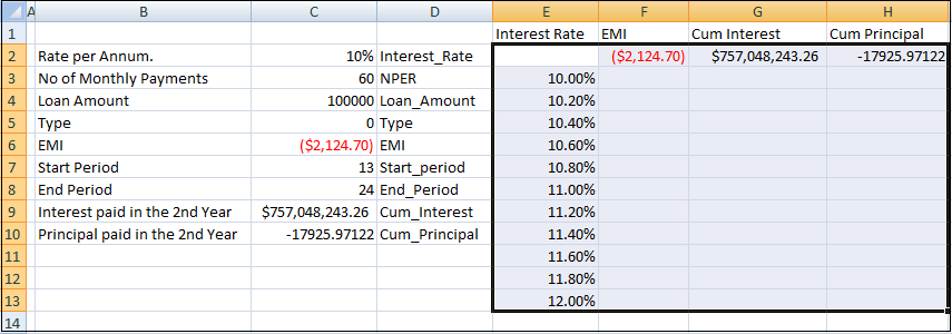
Step 5: Select the range of cells that contains the formulas and values that you want to substitute, E2:H13.
Step 6: Go to the Data tab, select What-if Analysis and click on the Data Table tool in the dropdown list.
Step 7: Data Table dialog box appears.
- Click in the Column input cell box.
- And click on the Interest_Rate cell, which is C2.
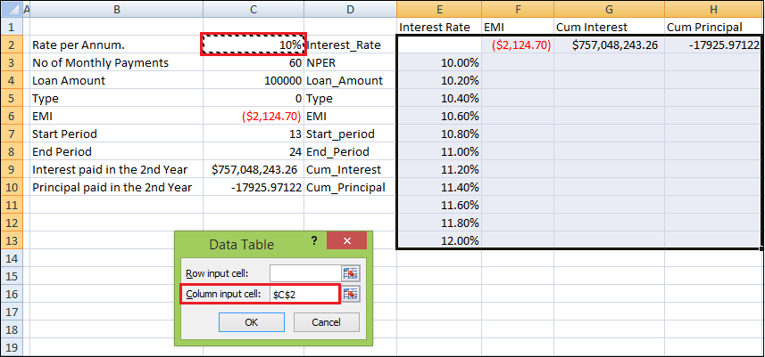
You can see that the Column input cell is taken as $C$2.
Step 8: Click on the Ok button.
The Data Table is filled with the calculated results for each input value.
Two-variable Data Tables
A two-variable Data Table can be used to see how different values of two variables in a formula will change that formula’s results. In other words, with a two-variable Data Table, you can determine how changing two inputs changes a single output.
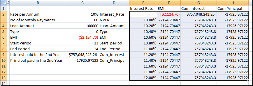
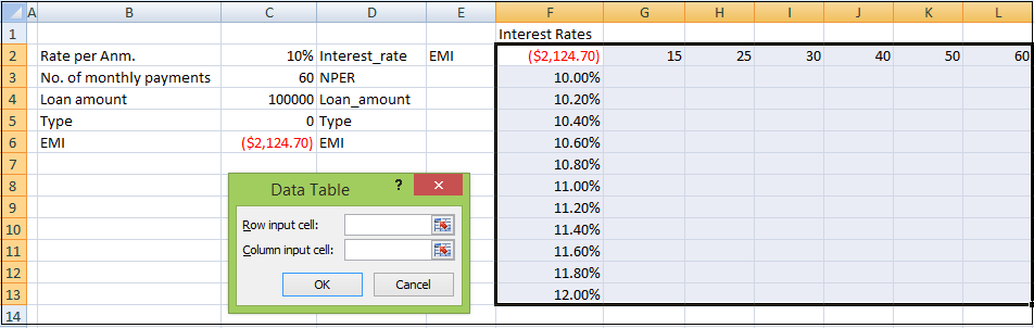
For example, a loan of 100000, and you want to know how different combinations of interest rates will affect the monthly payment.
Step 1: Create the following table.
Step 2: Now create the Data Table
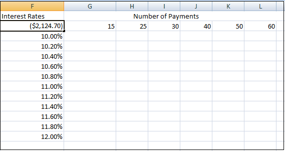
- Write =EMI in F2 cell.
- Type the first list of input values, i.e., interest rates, down the column F, starting with the cell below the formula, i.e., F3.
- Type the second list of input values, i.e., number of payments across row 2, starting with the cell to the right of the formula, i.e., G2.
- The Data Table looks as follows.
Step 3: Select the range of cells that contains the formula and the two sets of values that you want to substitute, i.e., F2:L13.
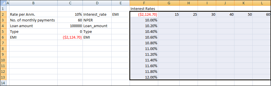
Step 4: Go to the Data tab, click What-if Analysis and select Data Table from the dropdown list.
Step 5: Data Table dialog box appears.
Step 6: Click in the Row input cell box.
- Click on the NPER cell, which is C3.
- Again, click in the Column input cell box.
- Click the Interest_Rate cell, which is C2.
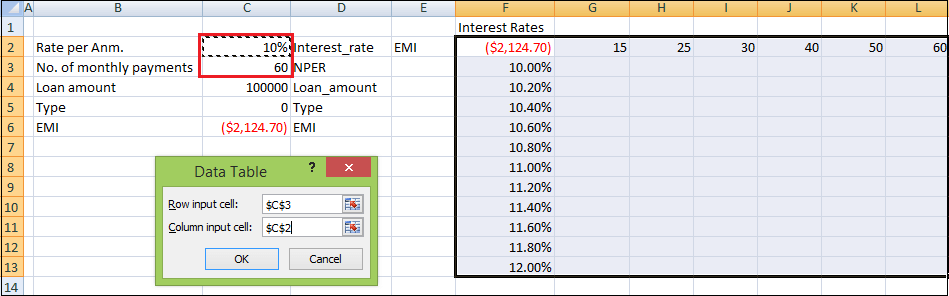
You will see that the Row input cell is taken as $C$3, and the Column input cell is taken as $C$2.
Step 7: Click on the Ok button.
The Data Table gets filled with the calculated results for each combination of the two input values.
Data Table Calculations
Data Tables are recalculated each time the worksheet containing them is recalculated, even if they have not changed.
To speed up the calculations in a worksheet that contains a Data Table, you need to change the calculation options to Automatically Recalculate the worksheet but not the Data Tables.
What If Analysis In Excel (Table of Contents)
- Overview of What-if Analysis in Excel
- Examples of What-if Analysis in Excel
Overview of What If Analysis in Excel
What-if analysis in Excel is used to test more than one value for a different formula on the basis of multiple scenarios. For this, we must have data of such kind where, for a single parameter, we would have 2 or more values for comparison. Go to the Data menu tab and click on the What-If Analysis option under the Forecast section. Select the scenario manager and give a scenario name and select the cell which contains the scenario value. By this, we can enter multiple scenarios. Now from the Goal Seek option from What-If Analysis, select the value we want to compare.
What if the analysis is available in the “forecast” section under the “Data” tab.
There are three different kinds of tolls in the What-if analysis. Those are:
1. Scenario manager
2. Goal Seek
3. Data table
We will see each one with related examples.
Examples of What If Analysis in Excel
Here are some examples given below:
You can download this What if Analysis Excel Template here – What if Analysis Excel Template
Example #1 – Scenario Manager
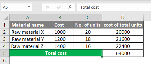
The scenario manager helps to find the results for different scenarios. Let’s consider a company that wants to buy raw materials for their organization’s needs. Due to the scarcity of funds, the company wants to understand how much cost will happen for different possibilities of buying.
In these cases, we can use the scenario manager for applying different scenarios to understand the results and make the decision accordingly. Now consider Raw material X, Raw material Y, and Raw material Z. We know the price of each, and we want to know how much amount need for different scenarios.
Now we need to design 3 scenarios like High volume purchase, Medium volume purchase, and Low volume purchase. For that, click on What if analysis and select Scenario manager.
Once we select the scenario manager, the following window will open.
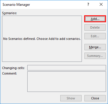
As shown in the screenshot, currently, there were no scenarios; if we want to add scenarios, we need to click on the “Add” option available.
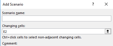
Then it will ask for the Scenario name and changing cells. Give scenario name whatever you want as per your requirement. Here I am giving “High volume.”
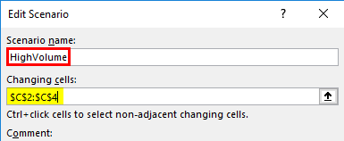
Changing cells is the range of cells that your scenario values for different scenarios. Suppose if we observe the below screenshot. No. of units will change in each scenario; that is the reason for changing cells; we used C2:C4, which means C2, C3, and C4.
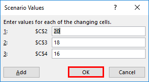
Once you give the change values, click on “OK”, then it will ask for the changing values for the High volume scenario. Input the values for high volume scenario and then click on “Add” to add another scenario “, Medium Volume.”
Give name as “Medium volume” and give the same range and click Ok then it will ask for values.
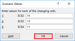
Again, click on “Add” and create one more scenario “, Low volume”, with low values like below.
Once all scenarios have done, click on “Ok” You will find the below screen.
We can find all the scenarios on the “Scenarios” screen. Now we can click on each scenario and click on Show; then you will find the results in excel; otherwise, we can view all the scenarios by clicking on the option “Summary.”
If we click on the scenario wise, the results will be changing in excel as below.
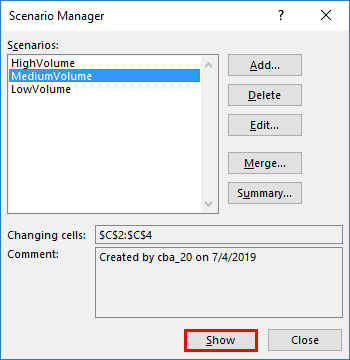
Whenever you click on the scenario and show the results at the back will change. If we want to see all the scenarios at a time to compare with others, click on the summary the following screen will come.
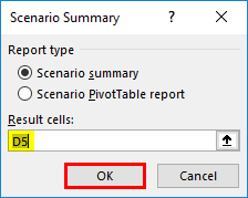
Select ‘Scenario Summary” and give the “Results Cells” here; the total results will be in D5; hence I given D5, click on ‘Ok’. Then a new tab will be created with the name “Scenario summary.”
Here the columns in grey color are the changing values, and the column in white color is the current value which was the last selected scenario results.
Example #2 – Goal Seek
Goal seek helps to find the input for the known output or required output.
Suppose we will take a small example of product sale. Suppose we know that we want to sell the product at an additional price of 200 than product cost then we want to know what is the percentage we are earning the profit.
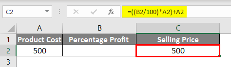
Observe the above screenshot product cost is 500, and I have given the formula for finding the percentage profit, which you can observe in the formula bar. In one more cell, I gave the formula for the additional price which we want to sell.
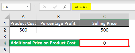
Now use Goal Seek to find the profit percentage of the different additional prices on the product’s product cost and selling price.
When we click on the “Goal seek”, the above pop up will come. In the set, the cell gives the cell position where we are going to give the output value here the additional price amount we know which we are giving in cell C4.
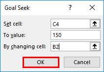
The “To Value” is the value at what additional price we want to cell 150 rupees additional to the product cost, and the changing cell is B2 where percentage changes. Click on “Ok” and see how much percentage profit if we sell an additional 150 rupees.
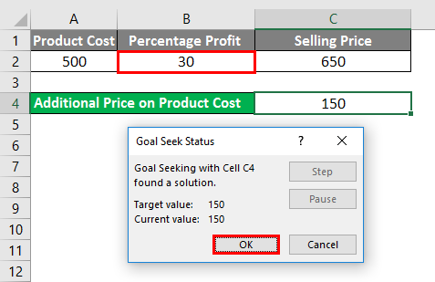
The profit percentage is 30, and the selling price should be 650. Similarly, we can check for different targeted values. This goal seeks to help to find the EMI calculations etc.
Example #3 – Data Tables in What If Analysis
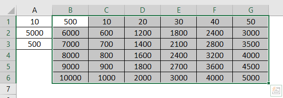
Now we will see the Data table. We will consider a very small example to understand better. Suppose we want to know the 10%, 20%, 30%, 40% and 50% of 5000 similarly, we want to find the percentages for 6000, 7000, 8000, 9000 and 10000.
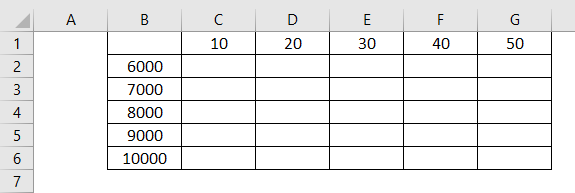
We have to get the percentages in each combination. In these situations, the Data table will help to find the output for a different combination of inputs. Here in Cell B3 should get 10% of 6000 and B4 10% of 7000 and so on. Now we will see how to achieve this. First, create a formula to perform this.
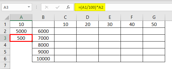
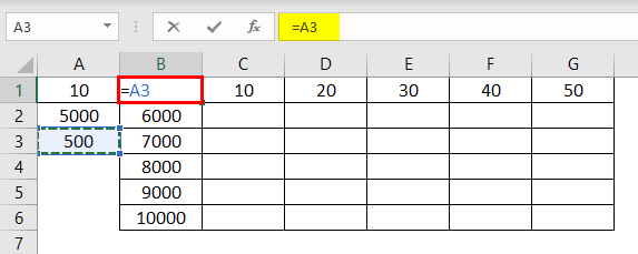
If we observe the above screenshot, the part marked with a box is the example. In A3, we have the formula to find the percentage from A1 and A2. So inputs are A1 and A2. Now take the result of A3 to A1 as shown in the below screenshot.
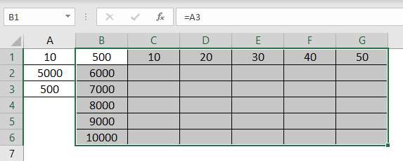
Now select the entire table to apply the Data table of What if Analysis as shown in the below screenshot.
Once selected, click on the “Data” then “What If Analysis” from that dropdown select data table.
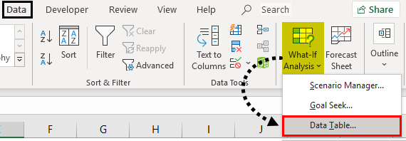
Once you select “Data table”, the below pop-up will come.
In “Row Input cell”, give the cell address where the row inputs should input, which means here row inputs are 10, 20, 30,40, and 50. Similarly, give “Column input cell” as A2 here column inputs are 6000, 7000, 8000, 9000, and 10,000. Click on “Ok”, then results will appear in the form of a table as shown below.
Things to Remember
- What if Analysis is available under the “Data” menu on the top.
- It will have 3 features 1. Scenario manager 2. Goal seeks and 3. Data table.
- Scenario manager helps to analyze different situations.
- Goal seek helps to know the right input value for the required output.
- Data table helps to get results of different inputs in row-wise and column-wise.
Recommended Articles
This is a guide on What if Analysis in Excel. Here we discuss three different tools in What if Analysis and the examples and downloadable excel template. You may also look at the following articles to learn more –
- Pareto Analysis in Excel
- Excel Quick Analysis
- Excel Regression Analysis
- Excel Tool for Data Analysis
This Excel tutorial explains how to use the Excel IF function with syntax and examples.
Description
The Microsoft Excel IF function returns one value if the condition is TRUE, or another value if the condition is FALSE.
The IF function is a built-in function in Excel that is categorized as a Logical Function. It can be used as a worksheet function (WS) in Excel. As a worksheet function, the IF function can be entered as part of a formula in a cell of a worksheet.
![]() Subscribe
Subscribe
If you want to follow along with this tutorial, download the example spreadsheet.
Download Example
Syntax
The syntax for the IF function in Microsoft Excel is:
IF( condition, value_if_true, [value_if_false] )
Parameters or Arguments
- condition
- The value that you want to test.
- value_if_true
- It is the value that is returned if condition evaluates to TRUE.
- value_if_false
- Optional. It is the value that is returned if condition evaluates to FALSE.
Returns
The IF function returns value_if_true when the condition is TRUE.
The IF function returns value_if_false when the condition is FALSE.
The IF function returns FALSE if the value_if_false parameter is omitted and the condition is FALSE.
Example (as Worksheet Function)
Let’s explore how to use the IF function as a worksheet function in Microsoft Excel.
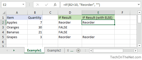
Based on the Excel spreadsheet above, the following IF examples would return:
=IF(B2<10, "Reorder", "")
Result: "Reorder"

=IF(A2="Apples", "Equal", "Not Equal")
Result: "Equal"

=IF(B3>=20, 12, 0)
Result: 12
Combining the IF function with Other Logical Functions
Quite often, you will need to specify more complex conditions when writing your formula in Excel. You can combine the IF function with other logical functions such as AND, OR, etc. Let’s explore this further.
AND function
The IF function can be combined with the AND function to allow you to test for multiple conditions. When using the AND function, all conditions within the AND function must be TRUE for the condition to be met. This comes in very handy in Excel formulas.
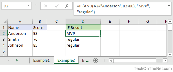
Based on the spreadsheet above, you can combine the IF function with the AND function as follows:
=IF(AND(A2="Anderson",B2>80), "MVP", "regular")
Result: "MVP"

=IF(AND(B2>=80,B2<=100), "Great Score", "Not Bad")
Result: "Great Score"

=IF(AND(B3>=80,B3<=100), "Great Score", "Not Bad")
Result: "Not Bad"

=IF(AND(A2="Anderson",A3="Smith",A4="Johnson"), 100, 50)
Result: 100

=IF(AND(A2="Anderson",A3="Smith",A4="Parker"), 100, 50)
Result: 50
In the examples above, all conditions within the AND function must be TRUE for the condition to be met.
OR function
The IF function can be combined with the OR function to allow you to test for multiple conditions. But in this case, only one or more of the conditions within the OR function needs to be TRUE for the condition to be met.
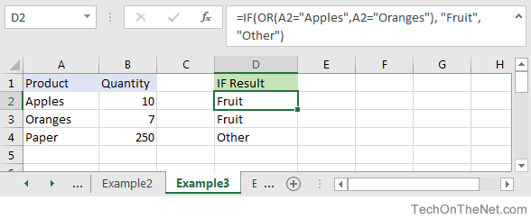
Based on the spreadsheet above, you can combine the IF function with the OR function as follows:
=IF(OR(A2="Apples",A2="Oranges"), "Fruit", "Other")
Result: "Fruit"

=IF(OR(A4="Apples",A4="Oranges"),"Fruit","Other")
Result: "Other"

=IF(OR(A4="Bananas",B4>=100), 999, "N/A")
Result: 999

=IF(OR(A2="Apples",A3="Apples",A4="Apples"), "Fruit", "Other")
Result: "Fruit"
In the examples above, only one of the conditions within the OR function must be TRUE for the condition to be met.
Let’s take a look at one more example that involves ranges of percentages.
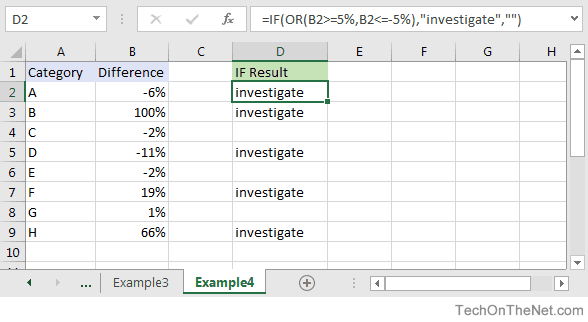
Based on the spreadsheet above, we would have the following formula in cell D2:
=IF(OR(B2>=5%,B2<=-5%),"investigate","")
Result: "investigate"
This IF function would return «investigate» if the value in cell B2 was either below -5% or above 5%. Since -6% is below -5%, it will return «investigate» as the result. We have copied this formula into cells D3 through D9 to show you the results that would be returned.
For example, in cell D3, we would have the following formula:
=IF(OR(B3>=5%,B3<=-5%),"investigate","")
Result: "investigate"
This formula would also return «investigate» but this time, it is because the value in cell B3 is greater than 5%.
Frequently Asked Questions
Question: In Microsoft Excel, I’d like to use the IF function to create the following logic:
if C11>=620, and C10=»F»or»S», and C4<=$1,000,000, and C4<=$500,000, and C7<=85%, and C8<=90%, and C12<=50, and C14<=2, and C15=»OO», and C16=»N», and C19<=48, and C21=»Y», then reference cell A148 on Sheet2. Otherwise, return an empty string.
Answer: The following formula would accomplish what you are trying to do:
=IF(AND(C11>=620, OR(C10="F",C10="S"), C4<=1000000, C4<=500000, C7<=0.85, C8<=0.9, C12<=50, C14<=2, C15="OO", C16="N", C19<=48, C21="Y"), Sheet2!A148, "")
Question: In Microsoft Excel, I’m trying to use the IF function to return 0 if cell A1 is either < 150,000 or > 250,000. Otherwise, it should return A1.
Answer: You can use the OR function to perform an OR condition in the IF function as follows:
=IF(OR(A1<150000,A1>250000),0,A1)
In this example, the formula will return 0 if cell A1 was either less than 150,000 or greater than 250,000. Otherwise, it will return the value in cell A1.
Question: In Microsoft Excel, I’m trying to use the IF function to return 25 if cell A1 > 100 and cell B1 < 200. Otherwise, it should return 0.
Answer: You can use the AND function to perform an AND condition in the IF function as follows:
=IF(AND(A1>100,B1<200),25,0)
In this example, the formula will return 25 if cell A1 is greater than 100 and cell B1 is less than 200. Otherwise, it will return 0.
Question: In Microsoft Excel, I need to write a formula that works this way:
IF (cell A1) is less than 20, then times it by 1,
IF it is greater than or equal to 20 but less than 50, then times it by 2
IF its is greater than or equal to 50 and less than 100, then times it by 3
And if it is great or equal to than 100, then times it by 4
Answer: You can write a nested IF statement to handle this. For example:
=IF(A1<20, A1*1, IF(A1<50, A1*2, IF(A1<100, A1*3, A1*4)))
Question: In Microsoft Excel, I need a formula in cell C5 that does the following:
IF A1+B1 <= 4, return $20
IF A1+B1 > 4 but <= 9, return $35
IF A1+B1 > 9 but <= 14, return $50
IF A1+B1 >= 15, return $75
Answer: In cell C5, you can write a nested IF statement that uses the AND function as follows:
=IF((A1+B1)<=4,20,IF(AND((A1+B1)>4,(A1+B1)<=9),35,IF(AND((A1+B1)>9,(A1+B1)<=14),50,75)))
Question: In Microsoft Excel, I need a formula that does the following:
IF the value in cell A1 is BLANK, then return «BLANK»
IF the value in cell A1 is TEXT, then return «TEXT»
IF the value in cell A1 is NUMERIC, then return «NUM»
Answer: You can write a nested IF statement that uses the ISBLANK function, the ISTEXT function, and the ISNUMBER function as follows:
=IF(ISBLANK(A1)=TRUE,"BLANK",IF(ISTEXT(A1)=TRUE,"TEXT",IF(ISNUMBER(A1)=TRUE,"NUM","")))
Question: In Microsoft Excel, I want to write a formula for the following logic:
IF R1<0.3 AND R2<0.3 AND R3<0.42 THEN «OK» OTHERWISE «NOT OK»
Answer: You can write an IF statement that uses the AND function as follows:
=IF(AND(R1<0.3,R2<0.3,R3<0.42),"OK","NOT OK")
Question: In Microsoft Excel, I need a formula for the following:
IF cell A1= PRADIP then value will be 100
IF cell A1= PRAVIN then value will be 200
IF cell A1= PARTHA then value will be 300
IF cell A1= PAVAN then value will be 400
Answer: You can write an IF statement as follows:
=IF(A1="PRADIP",100,IF(A1="PRAVIN",200,IF(A1="PARTHA",300,IF(A1="PAVAN",400,""))))
Question: In Microsoft Excel, I want to calculate following using an «if» formula:
if A1<100,000 then A1*.1% but minimum 25
and if A1>1,000,000 then A1*.01% but maximum 5000
Answer: You can write a nested IF statement that uses the MAX function and the MIN function as follows:
=IF(A1<100000,MAX(25,A1*0.1%),IF(A1>1000000,MIN(5000,A1*0.01%),""))
Question: In Microsoft Excel, I am trying to create an IF statement that will repopulate the data from a particular cell if the data from the formula in the current cell equals 0. Below is my attempt at creating an IF statement that would populate the data; however, I was unsuccessful.
=IF(IF(ISERROR(M24+((L24-S24)/AA24)),"0",M24+((L24-S24)/AA24)))=0,L24)
The initial part of the formula calculates the EAC (Estimate At completion = AC+(BAC-EV)/CPI); however if the current EV (Earned Value) is zero, the EAC will equal zero. IF the outcome is zero, I would like the BAC (Budget At Completion), currently recorded in another cell (L24), to be repopulated in the current cell as the EAC.
Answer: You can write an IF statement that uses the OR function and the ISERROR function as follows:
=IF(OR(S24=0,ISERROR(M24+((L24-S24)/AA24))),L24,M24+((L24-S24)/AA24))
Question: I have been looking at your Excel IF, AND and OR sections and found this very helpful, however I cannot find the right way to write a formula to express if C2 is either 1,2,3,4,5,6,7,8,9 and F2 is F and F3 is either D,F,B,L,R,C then give a value of 1 if not then 0. I have tried many formulas but just can’t get it right, can you help please?
Answer: You can write an IF statement that uses the AND function and the OR function as follows:
=IF(AND(C2>=1,C2<=9, F2="F",OR(F3="D",F3="F",F3="B",F3="L",F3="R",F3="C")),1,0)
Question:In Excel, I have a roadspeed of a car in m/s in cell A1 and a drop down menu of different units in C1 (which unclude mph and kmh). I have used the following IF function in B1 to convert the number to the unit selected from the dropdown box:
=IF(C1="mph","=A1*2.23693629",IF(C1="kmh","A1*3.6"))
However say if kmh was selected B1 literally just shows A1*3.6 and does not actually calculate it. Is there away to get it to calculate it instead of just showing the text message?
Answer: You are very close with your formula. Because you are performing mathematical operations (such as A1*2.23693629 and A1*3.6), you do not need to surround the mathematical formulas in quotes. Quotes are necessary when you are evaluating strings, not performing math.
Try the following:
=IF(C1="mph",A1*2.23693629,IF(C1="kmh",A1*3.6))
Question:For an IF statement in Excel, I want to combine text and a value.
For example, I want to put an equation for work hours and pay. IF I am paid more than I should be, I want it to read how many hours I owe my boss. But if I work more than I am paid for, I want it to read what my boss owes me (hours*Pay per Hour).
I tried the following:
=IF(A2<0,"I owe boss" abs(A2) "Hours","Boss owes me" abs(A2)*15 "dollars")
Is it possible or do I have to do it in 2 separate cells? (one for text and one for the value)
Answer: There are two ways that you can concatenate text and values. The first is by using the & character to concatenate:
=IF(A2<0,"I owe boss " & ABS(A2) & " Hours","Boss owes me " & ABS(A2)*15 & " dollars")
Or the second method is to use the CONCATENATE function:
=IF(A2<0,CONCATENATE("I owe boss ", ABS(A2)," Hours"), CONCATENATE("Boss owes me ", ABS(A2)*15, " dollars"))
Question:I have Excel 2000. IF cell A2 is greater than or equal to 0 then add to C1. IF cell B2 is greater than or equal to 0 then subtract from C1. IF both A2 and B2 are blank then equals C1. Can you help me with the IF function on this one?
Answer: You can write a nested IF statement that uses the AND function and the ISBLANK function as follows:
=IF(AND(ISBLANK(A2)=FALSE,A2>=0),C1+A2, IF(AND(ISBLANK(B2)=FALSE,B2>=0),C1-B2, IF(AND(ISBLANK(A2)=TRUE, ISBLANK(B2)=TRUE),C1,"")))
Question:How would I write this equation in Excel? IF D12<=0 then D12*L12, IF D12 is > 0 but <=600 then D12*F12, IF D12 is >600 then ((600*F12)+((D12-600)*E12))
Answer: You can write a nested IF statement as follows:
=IF(D12<=0,D12*L12,IF(D12>600,((600*F12)+((D12-600)*E12)),D12*F12))
Question:In Excel, I have this formula currently:
=IF(OR(A1>=40, B1>=40, C1>=40), "20", (A1+B1+C1)-20)
If one of my salesman does sale for $40-$49, then his commission is $20; however if his/her sale is less (for example $35) then the commission is that amount minus $20 ($35-$20=$15). I have 3 columns that are needed based on the type of sale. Only one column per row will be needed. The problem is that, when left blank, the total in the formula cell is -20. I need help setting up this formula so that when the 3 columns are left blank, the cell with the formula is left blank as well.
Answer: Using the AND function and the ISBLANK function, you can write your IF statement as follows:
=IF(AND(ISBLANK(A1),ISBLANK(B1),ISBLANK(C1)),"",IF(OR(A1>40, B1>40, C1>40), "20", (A1+B1+C1)-20))
In this formula, we are using the ISBLANK function to check if all 3 cells A1, B1, and C1 are blank, and if they are return a blank value («»). Then the rest is the formula that you originally wrote.
Question:In Excel, I need to create a simple booking and and out system, that shows a date out and a date back
«A1» = allows person to input date booked out
«A2» =allows person to input date booked back in
«A3″= shows status of product, eg, booked out, overdue return etc.
I can automate A3 with the following IF function:
=IF(ISBLANK(A2),"booked out","returned")
But what I cant get to work is if the product is out for 10 days or more, I would like the cell to say «send email»
Can you assist?
Answer: Using the TODAY function and adding an additional IF function, you can write your formula as follows:
=IF(ISBLANK(A2),IF(TODAY()-A1>10,"send email","booked out"),"returned")
Question:Using Microsoft Excel, I need a formula in cell U2 that does the following:
IF the date in E2<=12/31/2010, return T2*0.75
IF the date in E2>12/31/2010 but <=12/31/2011, return T2*0.5
IF the date in E2>12/31/2011, return T2*0
I tried using the following formula, but it gives me «#VALUE!»
=IF(E2<=DATE(2010,12,31),T2*0.75), IF(AND(E2>DATE(2010,12,31),E2<=DATE(2011,12,31)),T2*0.5,T2*0)
Can someone please help? Thanks.
Answer: You were very close…you just need to adjust your parentheses as follows:
=IF(E2<=DATE(2010,12,31),T2*0.75, IF(AND(E2>DATE(2010,12,31),E2<=DATE(2011,12,31)),T2*0.5,T2*0))
Question:In Excel, I would like to add 60 days if grade is ‘A’, 45 days if grade is ‘B’ and 30 days if grade is ‘C’. It would roughly look something like this, but I’m struggling with commas, brackets, etc.
(IF C5=A)=DATE(YEAR(B5)+0,MONTH(B5)+0,DAY(B5)+60),
(IF C5=B)=DATE(YEAR(B5)+0,MONTH(B5)+0,DAY(B5)+45),
(IF C5=C)=DATE(YEAR(B5)+0,MONTH(B5)+0,DAY(B5)+30)
Answer:You should be able to achieve your date calculations with the following formula:
=IF(C5="A",B5+60,IF(C5="B",B5+45,IF(C5="C",B5+30)))
Question:In Excel, I am trying to write a function and can’t seem to figure it out. Could you help?
IF D3 is < 31, then 1.51
IF D3 is between 31-90, then 3.40
IF D3 is between 91-120, then 4.60
IF D3 is > 121, then 5.44
Answer:You can write your formula as follows:
=IF(D3>121,5.44,IF(D3>=91,4.6,IF(D3>=31,3.4,1.51)))
Question:I would like ask a question regarding the IF statement. How would I write in Excel this problem?
I have to check if cell A1 is empty and if not, check if the value is less than equal to 5. Then multiply the amount entered in cell A1 by .60. The answer will be displayed on Cell A2.
Answer:You can write your formula in cell A2 using the IF function and ISBLANK function as follows:
=IF(AND(ISBLANK(A1)=FALSE,A1<=5),A1*0.6,"")
Question:In Excel, I’m trying to nest an OR command and I can’t find the proper way to write it. I want the spreadsheet to do the following:
If D6 equals «HOUSE» and C6 equals either «MOUSE» or «CAT», I want to return the value in cell B6. Otherwise, the formula should return the value «BLANK».
I tried the following:
=IF((D6="HOUSE")*(C6="MOUSE")*OR(C6="CAT"));B6;"BLANK")
If I only ask for HOUSE and MOUSE or HOUSE and CAT, it works, but as soon as I ask for MOUSE OR CAT, it doesn’t work.
Answer:You can write your formula using the AND function and OR function as follows:
=IF(AND(D6="HOUSE",OR(C6="MOUSE",C6="CAT")),B6,"BLANK")
This will return the value in B6 if D6 equals «HOUSE» and C6 equals either «MOUSE» or «CAT». If those conditions are not met, the formula will return the text value of «BLANK».
Question:In Microsoft Excel, I’m trying to write the following formula:
If cell A1 equals «jaipur», «udaipur» or «jodhpur», then cell A2 should display «rajasthan»
If cell A1 equals «bangalore», «mysore» or «belgum», then cell A2 should display «karnataka»
Please help.
Answer:You can write your formula using the OR function as follows:
=IF(OR(A1="jaipur",A1="udaipur",A1="jodhpur"),"rajasthan", IF(OR(A1="bangalore",A1="mysore",A1="belgum"),"karnataka"))
This will return «rajasthan» if A1 equals either «jaipur», «udaipur» or «jodhpur» and it will return «karnataka» if A1 equals either «bangalore», «mysore» or «belgum».
Question:In Microsoft Excel I’m trying to achieve the following with IF function:
If a value in any cell in column F is «food» then add the value of its corresponding cell in column G (eg a corresponding cell for F3 is G3). The IF function is performed in another cell altogether. I can do it for a single pair of cells but I don’t know how to do it for an entire column. Could you help?
At the moment, I’ve got this:
=IF(F3="food"; G3; 0)
Answer:This formula can be created using the SUMIF formula instead of using the IF function:
=SUMIF(F1:F10,"=food",G1:G10)
This will evaluate the first 10 rows of data in your spreadsheet. You may need to adjust the ranges accordingly.
I notice that you separate your parameters with semi-colons, so you might need to replace the commas in the formula above with semi-colons.
Question:I’m looking for an Exel formula that says:
If F3 is «H» and E3 is «H», return 1
If F3 is «A» and E3 is «A», return 2
If F3 is «d» and E3 is «d», return 3
Appreciate if you can help.
Answer:This Excel formula can be created using the AND formula in combination with the IF function:
=IF(AND(F3="H",E3="H"),1,IF(AND(F3="A",E3="A"),2,IF(AND(F3="d",E3="d"),3,"")))
We’ve defaulted the formula to return a blank if none of the conditions above are met.
Question:I am trying to get Excel to check different boxes and check if there is text/numbers listed in the cells and then spit out «Complete» if all 5 Boxes have text/Numbers or «Not Complete» if one or more is empty. This is what I have so far and it doesn’t work.
=IF(OR(ISBLANK(J2),ISBLANK(M2),ISBLANK(R2),ISBLANK (AA2),ISBLANK (AB2)),"Not Complete","")
Answer:First, you are correct in using the ISBLANK function, however, you have a space between ISBLANK and (AA2), as well as ISBLANK and (AB2). This might seem insignificant, but Excel can be very picky and will return a #NAME? error. So first you need to eliminate those spaces.
Next, you need to change the ELSE condition of your IF function to return «Complete».
You should be able to modify your formula as follows:
=IF(OR(ISBLANK(J2),ISBLANK(M2),ISBLANK(R2),ISBLANK(AA2),ISBLANK(AB2)), "Not Complete", "Complete")
Now if any of the cell J2, M2, R2, AA2, or AB2 are blank, the formula will return «Not Complete». If all 5 cells have a value, the formula will return «Complete».
Question:I’m very new to the Excel world, and I’m trying to figure out how to set up the proper formula for an If/then cell.
What I’m trying for is:
If B2’s value is 1 to 5, then multiply E2 by .77
If B2’s value is 6 to 10, then multiply E2 by .735
If B2’s value is 11 to 19, then multiply E2 by .7
If B2’s value is 20 to 29, then multiply E2 by .675
If B2’s value is 30 to 39, then multiply E2 by .65
I’ve tried a few different things thinking I was on the right track based on the IF, and AND function tutorials here, but I can’t seem to get it right.
Answer:To write your IF formula, you need to nest multiple IF functions together in combination with the AND function.
The following formula should work for what you are trying to do:
=IF(AND(B2>=1, B2<=5), E2*0.77, IF(AND(B2>=6, B2<=10), E2*0.735, IF(AND(B2>=11, B2<=19), E2*0.7, IF(AND(B2>=20, B2<=29), E2*0.675, IF(AND(B2>=30, B2<=39), E2*0.65,"")))))
As one final component of your formula, you need to decide what to do when none of the conditions are met. In this example, we have returned «» when the value in B2 does not meet any of the IF conditions above.
Question:Here is the Excel formula that has me between a rock and a hard place.
If E45 <= 50, return 44.55
If E45 > 50 and E45 < 100, return 42
If E45 >=200, return 39.6
Again thank you very much.
Answer:You should be able to write this Excel formula using a combination of the IF function and the AND function.
The following formula should work:
=IF(E45<=50, 44.55, IF(AND(E45>50, E45<100), 42, IF(E45>=200, 39.6, "")))
Please note that if none of the conditions are met, the Excel formula will return «» as the result.
Question:I have a nesting OR function problem:
My nonworking formula is:
=IF(C9=1,K9/J7,IF(C9=2,K9/J7,IF(C9=3,K9/L7,IF(C9=4,0,K9/N7))))
In Cell C9, I can have an input of 1, 2, 3, 4 or 0. The problem is on how to write the «or» condition when a «4 or 0» exists in Column C. If the «4 or 0» conditions exists in Column C I want Column K divided by Column N and the answer to be placed in Column M and associated row
Answer:You should be able to use the OR function within your IF function to test for C9=4 OR C9=0 as follows:
=IF(C9=1,K9/J7,IF(C9=2,K9/J7,IF(C9=3,K9/L7,IF(OR(C9=4,C9=0),K9/N7))))
This formula will return K9/N7 if cell C9 is either 4 or 0.
Question:In Excel, I am trying to create a formula that will show the following:
If column B = Ross and column C = 8 then in cell AB of that row I want it to show 2013, If column B = Block and column C = 9 then in cell AB of that row I want it to show 2012.
Answer:You can create your Excel formula using nested IF functions with the AND function.
=IF(AND(B1="Ross",C1=8),2013,IF(AND(B1="Block",C1=9),2012,""))
This formula will return 2013 as a numeric value if B1 is «Ross» and C1 is 8, or 2012 as a numeric value if B1 is «Block» and C1 is 9. Otherwise, it will return blank, as denoted by «».
Question:In Excel, I really have a problem looking for the right formula to express the following:
If B1=0, C1 is equal to A1/2
If B1=1, C1 is equal to A1/2 times 20%
If D1=1, C1 is equal to A1/2-5
I’ve been trying to look for any same expressions in your site. Please help me fix this.
Answer:In cell C1, you can use the following Excel formula with 3 nested IF functions:
=IF(B1=0,A1/2, IF(B1=1,(A1/2)*0.2, IF(D1=1,(A1/2)-5,"")))
Please note that if none of the conditions are met, the Excel formula will return «» as the result.
Question:In Excel, I need the answer for an IF THEN statement which compares column A and B and has an «OR condition» for column C. My problem is I want column D to return yes if A1 and B1 are >=3 or C1 is >=1.
Answer:You can create your Excel IF formula as follows:
=IF(OR(AND(A1>=3,B1>=3),C1>=1),"yes","")
Please note that if none of the conditions are met, the Excel formula will return «» as the result.
Question:In Excel, what have I done wrong with this formula?
=IF(OR(ISBLANK(C9),ISBLANK(B9)),"",IF(ISBLANK(C9),D9-TODAY(), "Reactivated"))
I want to make an event that if B9 and C9 is empty, the value would be empty. If only C9 is empty, then the output would be the remaining days left between the two dates, and if the two cells are not empty, the output should be the string ‘Reactivated’.
The problem with this code is that IF(ISBLANK(C9),D9-TODAY() is not working.
Answer:First of all, you might want to replace your OR function with the AND function, so that your Excel IF formula looks like this:
=IF(AND(ISBLANK(C9),ISBLANK(B9)),"",IF(ISBLANK(C9),D9-TODAY(),"Reactivated"))
Next, make sure that you don’t have any abnormal formatting in the cell that contains the results. To be safe, right click on the cell that contains the formula and choose Format Cells from the popup menu. When the Format Cells window appears, select the Number tab. Choose General as the format and click on the OK button.
Question:I was wondering if you could tell me what I am doing wrong.
Here are the instructions:
A customer is eligible for a discount if the customer’s 2016 sales greater than or equal to 100000 OR if the customers First Order was placed in 2016.
If the customer qualifies for a discount, return a value of Y
If the customer does not qualify for a discount, return a value of N.
Here is the formula I’ve entered:
=IF(OR([2014 Sales]=0,[2015 Sales]=0,[2016 Sales]>=100000),"Y","N")
I only have 2 cells wrong. Can you help me please? I am very lost and confused.
Answer:You are very close with your IF formula, however, it looks like you need to add the AND function to your formula as follows:
=IF(OR([2016 Sales]>=100000,AND([2014 Sales]=0,[2015 Sales]=0),C8>=100000),"Y","N")
This formula should return Y if 2016 sales are greater than or equal to 100000, or if both 2014 sales and 2015 sales are 0. Otherwise, the formula will return N. You will also notice that we switched the order of your conditions in the formula so that it is easier to understand the formula based on your instructions above.
Question:Could you please help me? I need to use «OR» on my formula but I can’t get it to work. This is what I’ve tried:
=IF(C6>=0<=150,150000,IF(C6>=151<=160,158400))
Here is what I need the formula to do:
IF C6 IS >=0 OR <=150 THEN ASSIGN $150000
IF C6 IS >=151 OR <=160 THEN ASSIGN $158400
Answer:You should be able to use the AND function within your IF function as follows:
=IF(AND(ISBLANK(C6)=FALSE,C6>=0,C6<=150),150000,IF(AND(C6>=151,C6<=160),158400,""))
Notice that we first use the ISBLANK function to test C6 to make sure that it is not blank. This is because if C6 if blank, it will evalulate to greater than 0 and thus return 150000. To avoid this, we include ISBLANK(C6)=FALSE as one of the conditions in addition to C6>=0 and C6<=150. That way, you won’t return any false results if C6 is blank.
Question:I am having a problem with a formula, I want it to be IF E5=N then do the first formula, else do the second formula. Excel recognizes the =IF(logical_test,value_if_TRUE,value_if_FALSE) but doesn’t like the formula below:
=IF(e5="N",((AND(AH5-AG5<456, AH5-S5<822)), "Compliant", "not Compliant"),((AH5-S5<822), "Compliant", "not Compliant"))
Any help would be greatly appreciated.
Answer:To have the first formula executed when E5=N and then second formula executed when E5<>N, you will need to nest 2 additional IF functions within the main IF function as follows:
=IF(E5="N", IF((AND(AH5-AG5<456, AH5-S5<822)), "Compliant", "not Compliant"), IF((AH5-S5<822), "Compliant", "not Compliant"))
If E5=»N», the first nested IF function will be executed:
IF((AND(AH5-AG5<456, AH5-S5<822)), "Compliant", "not Compliant")
Otherwise,the second nested IF function will be executed:
IF((AH5-S5<822), "Compliant", "not Compliant"))
Question:I need to write a formula based on the following logic:
There is a maximum discount allowed of £1000 if the capital sum is less that £43000 and a lower discount of £500 if the capital sum is above £43000. So the formula should return either £500 or £1000 in the cell but the £43000 is made up of two numbers, say for e.g. £42750+350 and if the second number is less than the allowed discount, the actual lower value is returned — in this case the £500 or £1000 becomes £350. Or as another e.g. £42000+750 returns £750.
So on my spreadsheet, in this second e.g. I would have A1= £42000, A2=750, A3=A1+A2, A4=the formula with the changing discount, in this case £750.
How can I write this formula?
Answer:In cell A4, you can calculate the correct discount using the IF function and the MIN function as follows:
=IF(A3<43000, MIN(A2,1000), MIN(A2,500))
If A3 is less than 43000, the formula will return the lower value of A2 and 1000. Otherwise, it will return the lower value of A2 and 500.
Question: I have a list of sizes in column A with sizes 100, 200, 300, 400, 500, 600. Then I have another column B, with sizes of my products, and it is random, for example, 318, 445, 527. What I’m trying to create is for a value of 318 in column B, I need to return 400 for that product. If the value in column B is 445, then I should return 500 and so on, as long sizes in column A must be BIGGER to the NEAREST size to column B.
Any idea how to create this function?
Answer:If your sizes are in increments of 100, you can create this function by taking the value in column B, dividing by 100, rounding up to the nearest integer, and then multiplying by 100.
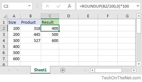
For example in cell C2, you can use the IF function and the ROUNDUP function as follows:
=ROUNDUP(B2/100,0)*100
This will return the correct value of 400 for a value of 318 in cell B2. Just copy this formula to cell C3, C4 and so on.
The IF function runs a logical test and returns one value for a TRUE result, and another value for a FALSE result. The result from IF can be a value, a cell reference, or even another formula. By combining the IF function with other logical functions like AND and OR, you can test more than one condition at a time.
Syntax
The generic syntax for the IF function looks like this:
=IF(logical_test,[value_if_true],[value_if_false])The first argument, logical_test, is typically an expression that returns either TRUE or FALSE. The second argument, value_if_true, is the value to return when logical_test is TRUE. The last argument, value_if_false, is the value to return when logical_test is FALSE. Both value_if_true and value_if_false are optional, but you must provide one or the other. For example, if cell A1 contains 80, then:
=IF(A1>75,TRUE) // returns TRUE
=IF(A1>75,"OK") // returns "OK"
=IF(A1>85,"OK") // returns FALSE
=IF(A1>75,10,0) // returns 10
=IF(A1>85,10,0) // returns 0
=IF(A1>75,"Yes","No") // returns "Yes"
=IF(A1>85,"Yes","No") // returns "No"
Notice that text values like «OK», «Yes», «No», etc. must be enclosed in double quotes («»). However, numeric values should not be enclosed in quotes.
Logical tests
The IF function supports logical operators (>,<,<>,=) when creating logical tests. Most commonly, the logical_test in IF is a complete logical expression that will evaluate to TRUE or FALSE. The table below shows some common examples:
| Goal | Logical test |
|---|---|
| If A1 is greater than 75 | A1>75 |
| If A1 equals 100 | A1=100 |
| If A1 is less than or equal to 100 | A1<=100 |
| If A1 equals «Red» | A1=»red» |
| If A1 is not equal to «Red» | A1<>»red» |
| If A1 is less than B1 | A1<B1 |
| If A1 is empty | A1=»» |
| If A1 is not empty | A1<>»» |
| If A1 is less than current date | A1<TODAY() |
Notice text values must be enclosed in double quotes («»), but numbers do not. The IF function does not support wildcards, but you can combine IF with COUNTIF to get basic wildcard functionality. To test for substrings in a cell, you can use the IF function with the SEARCH function.
Pass or Fail example
In the worksheet shown above, we want to assign either «Pass» or «Fail» based on a test score. A passing score is 70 or higher. The formula in D6, copied down, is:
=IF(C5>=70,"Pass","Fail")
Translation: If the value in C5 is greater than or equal to 70, return «Pass». Otherwise, return «Fail».
Note that the logical flow of this formula can be reversed. This formula returns the same result:
=IF(C5<70,"Fail","Pass")
Translation: If the value in C5 is less than 70, return «Fail». Otherwise, return «Pass».
Both formulas above, when copied down, will return correct results.
Note: If you are new to the idea of formula criteria, this article explains many examples.
Assign points based on color
In the worksheet below, we want to assign points based on the color in column B. If the color is «red», the result should be 100. If the color is «blue», the result should be 125. This requires that we use a formula based on two IF functions, one nested inside the other. The formula in C5, copied down, is:
=IF(B5="red",100,IF(B5="blue",125))
Translation: IF the value in B5 is «red», return 100. Else, if the value in B5 is «blue», return 125.

There are three things to notice in this example:
- The formula will return FALSE if the value in B5 is anything except «red» or «blue»
- The text values «red» and «blue» must be enclosed in double quotes («»)
- The IF function is not case-sensitive and will match «red», «Red», «RED», or «rEd».
This is a simple example of a nested IFs formula. See below for a more complex example.
Return another formula
The IF function can return another formula as a result. For example, the formula below will return A1*5% when A1 is less than 100, and A1*7% when A1 is greater than or equal to 100:
=IF(A1<100,A1*5%,A1*7%)
Nested IF statements
The IF function can be «nested». A «nested IF» refers to a formula where at least one IF function is nested inside another in order to test for more conditions and return more possible results. Each IF statement needs to be carefully «nested» inside another so that the logic is correct. For example, the following formula can be used to assign a grade rather than a pass / fail result:
=IF(C6<70,"F",IF(C6<75,"D",IF(C6<85,"C",IF(C6<95,"B","A"))))
Up to 64 IF functions can be nested. However, in general, you should consider other functions, like VLOOKUP or XLOOKUP for more complex scenarios, because they can handle more conditions in a more streamlined fashion. For a more details see this article on nested IFs.
Note: the newer IFS function is designed to handle multiple conditions without nesting. However, a lookup function like VLOOKUP or XLOOKUP is usually a better approach unless the logic for each condition is custom.
IF with AND, OR, NOT
The IF function can be combined with the AND function and the OR function. For example, to return «OK» when A1 is between 7 and 10, you can use a formula like this:
=IF(AND(A1>7,A1<10),"OK","")
Translation: if A1 is greater than 7 and less than 10, return «OK». Otherwise, return nothing («»).
To return B1+10 when A1 is «red» or «blue» you can use the OR function like this:
=IF(OR(A1="red",A1="blue"),B1+10,B1)
Translation: if A1 is red or blue, return B1+10, otherwise return B1.
=IF(NOT(A1="red"),B1+10,B1)
Translation: if A1 is NOT red, return B1+10, otherwise return B1.
IF cell contains specific text
Because the IF function does not support wildcards, it is not obvious how to configure IF to check for a specific substring in a cell. A common approach is to combine the ISNUMBER function and the SEARCH function to create a logical test like this:
=ISNUMBER(SEARCH(substring,A1)) // returns TRUE or FALSEFor example, to check for the substring «xyz» in cell A1, you can use a formula like this:
=IF(ISNUMBER(SEARCH("xyz",A1)),"Yes","No")Read a detailed explanation here.
More information
- Read more about nested IFs
- Learn how to use VLOOKUP instead of nested IFs (video)
- 50 Examples of formula criteria
Notes
- The IF function is not case-sensitive.
- To count values conditionally, use the COUNTIF or the COUNTIFS functions.
- To sum values conditionally, use the SUMIF or the SUMIFS functions.
- If any of the arguments to IF are supplied as arrays, the IF function will evaluate every element of the array.
What-If analysis is the process of calculating backward to find out an input by providing a specific output. In other words, what-if analysis can be considered as opposite to formulas. You use formulas to calculate an output by providing inputs whereas what-if analysis helps you find out what input will result in a specific output.
You can use what-if analysis to estimate your monthly savings that meet your retirement goals, find the return on investment, plan your budget and so on.
What is What-If Analysis
There are three different tools available in Excel to perform what-if analysis: scenarios, data tables and Goal Seek.
Scenario Manager
Scenario Manager allows you to create and compare different scenarios based on different sets of input values. Here’s how to use it:
- Enter your data and formulas in the appropriate cells.
- Click on the Data tab in the Excel Ribbon, and then click on the What-If Analysis button.
- Select Scenario Manager from the drop-down menu.
- Click on the Add button to create a new scenario.
- In the Add Scenario dialog box, enter a name for the scenario and specify the input values you want to change.
- Click OK, and repeat the process for each additional scenario you want to create.
- To compare the scenarios, click on the Summary button in the Scenario Manager dialog box.
Data Tables
Data Tables allow you to see how changing two or more input values will affect the output value. Here’s how to use it:
- Enter your data and formulas in the appropriate cells.
- Click on the cell where you want to display the results of the data table.
- Click on the Data tab in the Excel Ribbon, and then click on the What-If Analysis button.
- Select Data Table from the drop-down menu.
- In the Data Table dialog box, specify the input values you want to change and the cell containing the formula you want to calculate.
- Click OK, and Excel will create a table showing how changing the input values will affect the output value.
Goal Seek
Let’s have a look at Goal Seek function.
Using Goal Seek function, you can change the data in formula and analyze how it affects the end result.
Have a look at the data given below (don’t get scared). We will be using this data to perform what-if analysis.
Example 1 Monthly EMI calculation
Suppose a person takes a loan for $25,000 from a bank at the interest rate of 20% per annum and he agrees to pay off the loan in one and a half years (18 months).
All remaining data including monthly EMI, monthly payment towards principal, monthly payment towards interest and remaining amount to be paid each month are calculated using financial formulas.

In this case, the person has to pay an amount of $1619.08 every month for 18 months to complete the loan. Assume that the person is capable of paying $2500 every month so that he can pay off the loan faster. So, how can we find out in how many months the person will be able to complete the loan if he pays $2500 monthly. Here comes Goal Seek function into picture.
Perform what-if analysis
Open Excel, copy the data shown above and save your file as what-if analysis.xlsx. Go to Data (main menu) —> What-If Analysis (in the Data Tools group) and select Goal Seek.

You will get a window like this:

Click in the textbox next to Set cell and click the cell E1 as we need to analyze the result by changing the monthly payment. In the To value: textbox, enter 2500 as this is our new value. After clicking in the By changing cell: textbox, click the cell B2 as we want to find out the change in number of payments (number of months). Now your window will look like this:

Click OK and now your screen will look like this:

If you analyze the value in cell B2, you could find that it is 11.03. It means that you can complete the loan in less than a year (in 11.03 months) if you make a payment of $2,500 per month.
Example 2 Notes average calculations
Suppose you are a student who plans to score an average of 80 in your semester exam. You scored 82, 70, 83 and 76 in the subjects English, Mathematics, Computer Science and Mechanics respectively. You have Statistics exam remaining and you want to calculate the marks you need to score in Statistics to achieve an average of 80. Your score sheet before the Statistics exam will be as follows:

Select the Goal Seek function to open the window. Click in the textbox next to Set cell: and click the cell that contains the average score (here the cell containing the value 77.5). In the To value: textbox, enter 80 as this is your target average.
After clicking in the By changing cell textbox, click the cell that will contain the score of Statistics (here the cell just above the cell with 77.5).
Click OK and your screen will look like this:

From this data it is clear that you have to score 89 in Statistics to achieve an overall average of 80. Similarly, you can use Goal Seek function in many different scenarios to analyze what input should be given in order to get a specific output.
In conclusion, What-If Analysis is a powerful feature in Microsoft Excel that enables users to explore different scenarios and see how changes in input values affect their data.
By using tools such as Goal Seek, Scenario Manager, and Data Tables, users can make informed decisions and improve their business or personal processes. Whether it’s finding the input value needed to achieve a specific outcome or comparing different scenarios based on different sets of input values, What-If Analysis helps users to understand the relationships between their data and make more accurate predictions about the future.
By mastering these tools, users can unlock the full potential of Excel and become more efficient and effective in their work.
Further reading:
Chart with a goal line
Adding average to the pivot table