
Excel for Microsoft 365 Excel 2021 Excel 2019 Excel 2016 Excel 2013 Excel 2010 Excel 2007 More…Less
Functions are predefined formulas that perform calculations by using specific values, called arguments, in a particular order, or structure. Functions can be used to perform simple or complex calculations. You can find all of Excel’s functions on the Formulas tab on the Ribbon:

-
Excel function syntax
The following example of the ROUND function rounding off a number in cell A10 illustrates a function’s syntax.

1. Structure. The structure of a function begins with an equal sign (=), followed by the function name, an opening parenthesis, the arguments for the function separated by commas, and a closing parenthesis.
2. Function name. For a list of available functions, click a cell and press SHIFT+F3, which will launch the Insert Function dialog.
3. Arguments. Arguments can be numbers, text, logical values such as TRUE or FALSE, arrays, error values such as #N/A, or cell references. The argument you designate must produce a valid value for that argument. Arguments can also be constants, formulas, or other functions.
4. Argument tooltip. A tooltip with the syntax and arguments appears as you type the function. For example, type =ROUND( and the tooltip appears. Tooltips appear only for built-in functions.
Note: You don’t need to type functions in all caps, like =ROUND, as Excel will automatically capitalize the function name for you once you press enter. If you misspell a function name, like =SUME(A1:A10) instead of =SUM(A1:A10), then Excel will return a #NAME? error.
-
Entering Excel functions
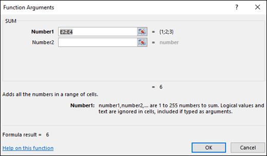
When you create a formula that contains a function, you can use the Insert Function dialog box to help you enter worksheet functions. Once you select a function from the Insert Function dialog Excel will launch a function wizard, which displays the name of the function, each of its arguments, a description of the function and each argument, the current result of the function, and the current result of the entire formula.
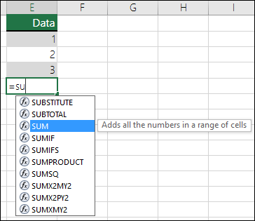
To make it easier to create and edit formulas and minimize typing and syntax errors, use Formula AutoComplete. After you type an = (equal sign) and beginning letters of a function, Excel displays a dynamic drop-down list of valid functions, arguments, and names that match those letters. You can then select one from the drop-down list and Excel will enter it for you.
-
Nesting Excel functions
In certain cases, you may need to use a function as one of the arguments of another function. For example, the following formula uses a nested AVERAGE function and compares the result with the value 50.
1. The AVERAGE and SUM functions are nested within the IF function.
Valid returns When a nested function is used as an argument, the nested function must return the same type of value that the argument uses. For example, if the argument returns a TRUE or FALSE value, the nested function must return a TRUE or FALSE value. If the function doesn’t, Excel displays a #VALUE! error value.
Nesting level limits A formula can contain up to seven levels of nested functions. When one function (we’ll call this Function B) is used as an argument in another function (we’ll call this Function A), Function B acts as a second-level function. For example, the AVERAGE function and the SUM function are both second-level functions if they are used as arguments of the IF function. A function nested within the nested AVERAGE function is then a third-level function, and so on.

Need more help?
Below is a brief overview of about 100 important Excel functions you should know, with links to detailed examples. We also have a large list of example formulas, a more complete list of Excel functions, and video training. If you are new to Excel formulas, see this introduction.
Note: Excel now includes Dynamic Array formulas, which offer important new functions.
Date and Time Functions
Excel provides many functions to work with dates and times.
NOW and TODAY
You can get the current date with the TODAY function and the current date and time with the NOW Function. Technically, the NOW function returns the current date and time, but you can format as time only, as seen below:

TODAY() // returns current date
NOW() // returns current time
Note: these are volatile functions and will recalculate with every worksheet change. If you want a static value, use date and time shortcuts.
DAY, MONTH, YEAR, and DATE
You can use the DAY, MONTH, and YEAR functions to disassemble any date into its raw components, and the DATE function to put things back together again.

=DAY("14-Nov-2018") // returns 14
=MONTH("14-Nov-2018") // returns 11
=YEAR("14-Nov-2018") // returns 2018
=DATE(2018,11,14) // returns 14-Nov-2018
HOUR, MINUTE, SECOND, and TIME
Excel provides a set of parallel functions for times. You can use the HOUR, MINUTE, and SECOND functions to extract pieces of a time, and you can assemble a TIME from individual components with the TIME function.

=HOUR("10:30") // returns 10
=MINUTE("10:30") // returns 30
=SECOND("10:30") // returns 0
=TIME(10,30,0) // returns 10:30
DATEDIF and YEARFRAC
You can use the DATEDIF function to get time between dates in years, months, or days. DATEDIF can also be configured to get total time in «normalized» denominations, i.e. «2 years and 6 months and 27 days».

Use YEARFRAC to get fractional years:

=YEARFRAC("14-Nov-2018","10-Jun-2021") // returns 2.57
EDATE and EOMONTH
A common task with dates is to shift a date forward (or backward) by a given number of months. You can use the EDATE and EOMONTH functions for this. EDATE moves by month and retains the day. EOMONTH works the same way, but always returns the last day of the month.

EDATE(date,6) // 6 months forward
EOMONTH(date,6) // 6 months forward (end of month)
WORKDAY and NETWORKDAYS
To figure out a date n working days in the future, you can use the WORKDAY function. To calculate the number of workdays between two dates, you can use NETWORKDAYS.

WORKDAY(start,n,holidays) // date n workdays in future
Video: How to calculate due dates with WORKDAY

NETWORKDAYS(start,end,holidays) // number of workdays between dates
Note: Both functions automatically skip weekends (Saturday and Sunday) and will also skip holidays, if provided. If you need more flexibility on what days are considered weekends, see the WORKDAY.INTL function and NETWORKDAYS.INTL function.
WEEKDAY and WEEKNUM
To figure out the day of week from a date, Excel provides the WEEKDAY function. WEEKDAY returns a number between 1-7 that indicates Sunday, Monday, Tuesday, etc. Use the WEEKNUM function to get the week number in a given year.

=WEEKDAY(date) // returns a number 1-7
=WEEKNUM(date) // returns week number in year
Engineering
CONVERT
Most Engineering functions are pretty technical…you’ll find a lot of functions for complex numbers in this section. However, the CONVERT function is quite useful for everyday unit conversions. You can use CONVERT to change units for distance, weight, temperature, and much more.

=CONVERT(72,"F","C") // returns 22.2
Information Functions
ISBLANK, ISERROR, ISNUMBER, and ISFORMULA
Excel provides many functions for checking the value in a cell, including ISNUMBER, ISTEXT, ISLOGICAL, ISBLANK, ISERROR, and ISFORMULA These functions are sometimes called the «IS» functions, and they all return TRUE or FALSE based on a cell’s contents.

Excel also has ISODD and ISEVEN functions that will test a number to see if it’s even or odd.
By the way, the green fill in the screenshot above is applied automatically with a conditional formatting formula.
Logical Functions
Excel’s logical functions are a key building block of many advanced formulas. Logical functions return the boolean values TRUE or FALSE. If you need a primer on logical formulas, this video goes through many examples.
AND, OR and NOT
The core of Excel’s logical functions are the AND function, the OR function, and the NOT function. In the screen below, each of these function is used to run a simple test on the values in column B:

=AND(B5>3,B5<9)
=OR(B5=3,B5=9)
=NOT(B5=2)
- Video: How to build logical formulas
- Guide: 50 examples of formula criteria
IFERROR and IFNA
The IFERROR function and IFNA function can be used as a simple way to trap and handle errors. In the screen below, VLOOKUP is used to retrieve cost from a menu item. Column F contains just a VLOOKUP function, with no error handling. Column G shows how to use IFNA with VLOOKUP to display a custom message when an unrecognized item is entered.

=VLOOKUP(E5,menu,2,0) // no error trapping
=IFNA(VLOOKUP(E5,menu,2,0),"Not found") // catch errors
Whereas IFNA only catches an #N/A error, the IFERROR function will catch any formula error.
IF and IFS functions
The IF function is one of the most used functions in Excel. In the screen below, IF checks test scores and assigns «pass» or «fail»:

Multiple IF functions can be nested together to perform more complex logical tests.
New in Excel 2019 and Excel 365, the IFS function can run multiple logical tests without nesting IFs.

=IFS(C5<60,"F",C5<70,"D",C5<80,"C",C5<90,"B",C5>=90,"A")
Lookup and Reference Functions
VLOOKUP and HLOOKUP
Excel offers a number of functions to lookup and retrieve data. Most famous of all is VLOOKUP:

=VLOOKUP(C5,$F$5:$G$7,2,TRUE)
More: 23 things to know about VLOOKUP.
HLOOKUP works like VLOOKUP, but expects data arranged horizontally:

=HLOOKUP(C5,$G$4:$I$5,2,TRUE)
INDEX and MATCH
For more complicated lookups, INDEX and MATCH offers more flexibility and power:

=INDEX(C5:E12,MATCH(H4,B5:B12,0),MATCH(H5,C4:E4,0))
Both the INDEX function and the MATCH function are powerhouse functions that turn up in all kinds of formulas.
More: How to use INDEX and MATCH
LOOKUP
The LOOKUP function has default behaviors that make it useful when solving certain problems. LOOKUP assumes values are sorted in ascending order and always performs an approximate match. When LOOKUP can’t find a match, it will match the next smallest value. In the example below we are using LOOKUP to find the last entry in a column:

ROW and COLUMN
You can use the ROW function and COLUMN function to find row and column numbers on a worksheet. Notice both ROW and COLUMN return values for the current cell if no reference is supplied:

The row function also shows up often in advanced formulas that process data with relative row numbers.
ROWS and COLUMNS
The ROWS function and COLUMNS function provide a count of rows in a reference. In the screen below, we are counting rows and columns in an Excel Table named «Table1».

Note ROWS returns a count of data rows in a table, excluding the header row. By the way, here are 23 things to know about Excel Tables.
HYPERLINK
You can use the HYPERLINK function to construct a link with a formula. Note HYPERLINK lets you build both external links and internal links:

=HYPERLINK(C5,B5)
GETPIVOTDATA
The GETPIVOTDATA function is useful for retrieving information from existing pivot tables.

=GETPIVOTDATA("Sales",$B$4,"Region",I6,"Product",I7)
CHOOSE
The CHOOSE function is handy any time you need to make a choice based on a number:

=CHOOSE(2,"red","blue","green") // returns "blue"
Video: How to use the CHOOSE function
TRANSPOSE
The TRANSPOSE function gives you an easy way to transpose vertical data to horizontal, and vice versa.

{=TRANSPOSE(B4:C9)}
Note: TRANSPOSE is a formula and is, therefore, dynamic. If you just need to do a one-time transpose operation, use Paste Special instead.
OFFSET
The OFFSET function is useful for all kinds of dynamic ranges. From a starting location, it lets you specify row and column offsets, and also the final row and column size. The result is a range that can respond dynamically to changing conditions and inputs. You can feed this range to other functions, as in the screen below, where OFFSET builds a range that is fed to the SUM function:

=SUM(OFFSET(B4,1,I4,4,1)) // sum of Q3
INDIRECT
The INDIRECT function allows you to build references as text. This concept is a bit tricky to understand at first, but it can be useful in many situations. Below, we are using INDIRECT to get values from cell A1 in 5 different worksheets. Each reference is dynamic. If a sheet name changes, the reference will update.

=INDIRECT(B5&"!A1") // =Sheet1!A1
The INDIRECT function is also used to «lock» references so they won’t change, when rows or columns are added or deleted. For more details, see linked examples at the bottom of the INDIRECT function page.
Caution: both OFFSET and INDIRECT are volatile functions and can slow down large or complicated spreadsheets.
STATISTICAL Functions
COUNT and COUNTA
You can count numbers with the COUNT function and non-empty cells with COUNTA. You can count blank cells with COUNTBLANK, but in the screen below we are counting blank cells with COUNTIF, which is more generally useful.

=COUNT(B5:F5) // count numbers
=COUNTA(B5:F5) // count numbers and text
=COUNTIF(B5:F5,"") // count blanks
COUNTIF and COUNTIFS
For conditional counts, the COUNTIF function can apply one criteria. The COUNTIFS function can apply multiple criteria at the same time:

=COUNTIF(C5:C12,"red") // count red
=COUNTIF(F5:F12,">50") // count total > 50
=COUNTIFS(C5:C12,"red",D5:D12,"TX") // red and tx
=COUNTIFS(C5:C12,"blue",F5:F12,">50") // blue > 50
Video: How to use the COUNTIF function
SUM, SUMIF, SUMIFS
To sum everything, use the SUM function. To sum conditionally, use SUMIF or SUMIFS. Following the same pattern as the counting functions, the SUMIF function can apply only one criteria while the SUMIFS function can apply multiple criteria.

=SUM(F5:F12) // everything
=SUMIF(C5:C12,"red",F5:F12) // red only
=SUMIF(F5:F12,">50") // over 50
=SUMIFS(F5:F12,C5:C12,"red",D5:D12,"tx") // red & tx
=SUMIFS(F5:F12,C5:C12,"blue",F5:F12,">50") // blue & >50
Video: How to use the SUMIF function
AVERAGE, AVERAGEIF, and AVERAGEIFS
Following the same pattern, you can calculate an average with AVERAGE, AVERAGEIF, and AVERAGEIFS.

=AVERAGE(F5:F12) // all
=AVERAGEIF(C5:C12,"red",F5:F12) // red only
=AVERAGEIFS(F5:F12,C5:C12,"red",D5:D12,"tx") // red and tx
MIN, MAX, LARGE, SMALL
You can find largest and smallest values with MAX and MIN, and nth largest and smallest values with LARGE and SMALL. In the screen below, data is the named range C5:C13, used in all formulas.

=MAX(data) // largest
=MIN(data) // smallest
=LARGE(data,1) // 1st largest
=LARGE(data,2) // 2nd largest
=LARGE(data,3) // 3rd largest
=SMALL(data,1) // 1st smallest
=SMALL(data,2) // 2nd smallest
=SMALL(data,3) // 3rd smallest
Video: How to find the nth smallest or largest value
MINIFS, MAXIFS
The MINIFS and MAXIFS. These functions let you find minimum and maximum values with conditions:

=MAXIFS(D5:D15,C5:C15,"female") // highest female
=MAXIFS(D5:D15,C5:C15,"male") // highest male
=MINIFS(D5:D15,C5:C15,"female") // lowest female
=MINIFS(D5:D15,C5:C15,"male") // lowest male
Note: MINIFS and MAXIFS are new in Excel via Office 365 and Excel 2019.
MODE
The MODE function returns the most commonly occurring number in a range:

=MODE(B5:G5) // returns 1
RANK
To rank values largest to smallest, or smallest to largest, use the RANK function:

Video: How to rank values with the RANK function
MATH Functions
ABS
To change negative values to positive use the ABS function.

=ABS(-134.50) // returns 134.50
RAND and RANDBETWEEN
Both the RAND function and RANDBETWEEN function can generate random numbers on the fly. RAND creates long decimal numbers between zero and 1. RANDBETWEEN generates random integers between two given numbers.

=RAND() // between zero and 1
=RANDBETWEEN(1,100) // between 1 and 100
ROUND, ROUNDUP, ROUNDDOWN, INT
To round values up or down, use the ROUND function. To force rounding up to a given number of digits, use ROUNDUP. To force rounding down, use ROUNDDOWN. To discard the decimal part of a number altogether, use the INT function.

=ROUND(11.777,1) // returns 11.8
=ROUNDUP(11.777) // returns 11.8
=ROUNDDOWN(11.777,1) // returns 11.7
=INT(11.777) // returns 11
MROUND, CEILING, FLOOR
To round values to the nearest multiple use the MROUND function. The FLOOR function and CEILING function also round to a given multiple. FLOOR forces rounding down, and CEILING forces rounding up.

=MROUND(13.85,.25) // returns 13.75
=CEILING(13.85,.25) // returns 14
=FLOOR(13.85,.25) // returns 13.75
MOD
The MOD function returns the remainder after division. This sounds boring and geeky, but MOD turns up in all kinds of formulas, especially formulas that need to do something «every nth time». In the screen below, you can see how MOD returns zero every third number when the divisor is 3:

SUMPRODUCT
The SUMPRODUCT function is a powerful and versatile tool when dealing with all kinds of data. You can use SUMPRODUCT to easily count and sum based on criteria, and you can use it in elegant ways that just don’t work with COUNTIFS and SUMIFS. In the screen below, we are using SUMPRODUCT to count and sum orders in March. See the SUMPRODUCT page for details and links to many examples.

=SUMPRODUCT(--(MONTH(B5:B12)=3)) // count March
=SUMPRODUCT(--(MONTH(B5:B12)=3),C5:C12) // sum March
SUBTOTAL
The SUBTOTAL function is an «aggregate function» that can perform a number of operations on a set of data. All told, SUBTOTAL can perform 11 operations, including SUM, AVERAGE, COUNT, MAX, MIN, etc. (see this page for the full list). The key feature of SUBTOTAL is that it will ignore rows that have been «filtered out» of an Excel Table, and, optionally, rows that have been manually hidden. In the screen below, SUBTOTAL is used to count and sum only the 7 visible rows in the table:

=SUBTOTAL(3,B5:B14) // returns 7
=SUBTOTAL(9,F5:F14) // returns 9.54
AGGREGATE
Like SUBTOTAL, the AGGREGATE function can also run a number of aggregate operations on a set of data and can optionally ignore hidden rows. The key differences are that AGGREGATE can run more operations (19 total) and can also ignore errors.
In the screen below, AGGREGATE is used to perform MIN, MAX, LARGE and SMALL operations while ignoring errors. Normally, the error in cell B9 would prevent these functions from returning a result. See this page for a full list of operations AGGREGATE can perform.

=AGGREGATE(4,6,values) // MAX ignore errors, returns 100
=AGGREGATE(5,6,values) // MIN ignore errors, returns 75
TEXT Functions
LEFT, RIGHT, MID
To extract characters from the left, right, or middle of text, use LEFT, RIGHT, and MID functions:

=LEFT("ABC-1234-RED",3) // returns "ABC"
=MID("ABC-1234-RED",5,4) // returns "1234"
=RIGHT("ABC-1234-RED",3) // returns "RED"
LEN
The LEN function will return the length of a text string. LEN shows up in a lot of formulas that count words or characters.

FIND, SEARCH
To look for specific text in a cell, use the FIND function or SEARCH function. These functions return the numeric position of matching text, but SEARCH allows wildcards and FIND is case-sensitive. Both functions will throw an error when text is not found, so wrap in the ISNUMBER function to return TRUE or FALSE (example here).

=FIND("Better the devil you know","devil") // returns 12
=SEARCH("This is not my beautiful wife","bea*") // returns 12
REPLACE, SUBSTITUTE
To replace text by position, use the REPLACE function. To replace text by matching, use the SUBSTITUTE function. In the first example, REPLACE removes the two asterisks (**) by replacing the first two characters with an empty string («»). In the second example, SUBSTITUTE removes all hash characters (#) by replacing «#» with «».

=REPLACE("**Red",1,2,"") // returns "Red"
=SUBSTITUTE("##Red##","#","") // returns "Red"
CODE, CHAR
To figure out the numeric code for a character, use the CODE function. To translate the numeric code back to a character, use the CHAR function. In the example below, CODE translates each character in column B to its corresponding code. In column F, CHAR translates the code back to a character.

=CODE("a") // returns 97
=CHAR(97) // returns "a"
Video: How to use the CODE and CHAR functions
TRIM, CLEAN
To get rid of extra space in text, use the TRIM function. To remove line breaks and other non-printing characters, use CLEAN.

=TRIM(A1) // remove extra space
=CLEAN(A1) // remove line breaks
Video: How to clean text with TRIM and CLEAN
CONCAT, TEXTJOIN, CONCATENATE
New in Excel via Office 365 are CONCAT and TEXTJOIN. The CONCAT function lets you concatenate (join) multiple values, including a range of values without a delimiter. The TEXTJOIN function does the same thing, but allows you to specify a delimiter and can also ignore empty values.

=TEXTJOIN(",",TRUE,B4:H4) // returns "red,blue,green,pink,black"
=CONCAT(B7:H7) // returns "8675309"
Excel also provides the CONCATENATE function, but it doesn’t offer special features. I wouldn’t bother with it and would instead concatenate directly with the ampersand (&) character in a formula.
EXACT
The EXACT function allows you to compare two text strings in a case-sensitive manner.

UPPER, LOWER, PROPER
To change the case of text, use the UPPER, LOWER, and PROPER function

=UPPER("Sue BROWN") // returns "SUE BROWN"
=LOWER("Sue BROWN") // returns "sue brown"
=PROPER("Sue BROWN") // returns "Sue Brown"
Video: How to change case with formulas
TEXT
Last but definitely not least is the TEXT function. The text function lets you apply number formatting to numbers (including dates, times, etc.) as text. This is especially useful when you need to embed a formatted number in a message, like «Sale ends on [date]».

=TEXT(B5,"$#,##0.00")
=TEXT(B6,"000000")
="Save "&TEXT(B7,"0%")
="Sale ends "&TEXT(B8,"mmm d")
More: Detailed examples of custom number formatting.
Dynamic Array functions
Dynamic arrays are new in Excel 365, and are a major upgrade to Excel’s formula engine. As part of the dynamic array update, Excel includes new functions which directly leverage dynamic arrays to solve problems that are traditionally hard to solve with conventional formulas. If you are using Excel 365, make sure you are aware of these new functions:
| Function | Purpose |
|---|---|
| FILTER | Filter data and return matching records |
| RANDARRAY | Generate array of random numbers |
| SEQUENCE | Generate array of sequential numbers |
| SORT | Sort range by column |
| SORTBY | Sort range by another range or array |
| UNIQUE | Extract unique values from a list or range |
| XLOOKUP | Modern replacement for VLOOKUP |
| XMATCH | Modern replacement for the MATCH function |
Video: New dynamic array functions in Excel (about 3 minutes).
Quick navigation
ABS, AGGREGATE, AND, AVERAGE, AVERAGEIF, AVERAGEIFS, CEILING, CHAR, CHOOSE, CLEAN, CODE, COLUMN, COLUMNS, CONCAT, CONCATENATE, CONVERT, COUNT, COUNTA, COUNTBLANK, COUNTIF, COUNTIFS, DATE, DATEDIF, DAY, EDATE, EOMONTH, EXACT, FIND, FLOOR, GETPIVOTDATA, HLOOKUP, HOUR, HYPERLINK, IF, IFERROR, IFNA, IFS, INDEX, INDIRECT, INT, ISBLANK, ISERROR, ISEVEN, ISFORMULA, ISLOGICAL, ISNUMBER, ISODD, ISTEXT, LARGE, LEFT, LEN, LOOKUP, LOWER, MATCH, MAX, MAXIFS, MID, MIN, MINIFS, MINUTE, MOD, MODE, MONTH, MROUND, NETWORKDAYS, NOT, NOW, OFFSET, OR, PROPER, RAND, RANDBETWEEN, RANK, REPLACE, RIGHT, ROUND, ROUNDDOWN, ROUNDUP, ROW, ROWS, SEARCH, SECOND, SMALL, SUBSTITUTE, SUBTOTAL, SUM, SUMIF, SUMIFS, SUMPRODUCT, TEXT, TEXTJOIN, TIME, TODAY, TRANSPOSE, TRIM, UPPER, VLOOKUP, WEEKDAY, WEEKNUM, WORKDAY, YEAR, YEARFRAC
The complete Excel Functions list includes lookup, logic, date and time, text, information, and math functions with examples. Excel Functions are built-in presets, so Excel functions are hard-coded formulas with short, user-friendly names.
The list contains 300+ built-in Excel functions. Furthermore, look at the library of useful advanced functions (UDFs). If you want to jump to a specific category, use the list below; else, use the Search box for the latest tutorials.
- User-defined functions (must-have)
- Logical
- Text
- Lookup
- Date and Time
- Dynamic array
- Information
- Math
- Statistical
- Financial
Excel Function List
Logical
The functions below use logical tests and logical operators to evaluate a formula. Learn more about Boolean expressions.
LOOKUP
Here is the list of lookup functions in Excel. Of course, we already know that XLOOKUP changes everything. But it is worth keeping in mind the older lookup functions too.
User-defined functions
UDFs are advanced functions.
Date and Time
Date and Time functions help you create calculations based on dates and times.
Text
Text functions in Excel enable you to perform various calculations using strings.
Dynamic Array
Dynamic Arrays are resizable arrays. From now, Excel calculates the array automatically and returns values into multiple cells based on a formula entered in a single cell.
Information
Take a quick overview of information functions in Excel.
Math
Math Functions are great.
Math – Part 2
Financial
Use financial functions if you want.
Financial – Part 2
Statistical
Statistical – Part 2
Trigonometry
Engineering
Database
How to use Excel Functions?
To use a function, type an equal sign (=) in the formula bar or the cell to enter a function you want to use. After that, enter the function’s name and the arguments. There are custom functions in Excel, user-defined functions. If you want to learn more about how to solve complex tasks using UDFs, read our guide.
15 Most Common Excel Functions You Must Know + How to Use Them
Microsoft Excel is one of the most well-known computer applications. It has changed the way people and companies work with data.
Thus, learning Excel can help with both your career and your personal needs.
Excel runs using functions and there are roughly 500 of them! These range from basic arithmetic to complex statistics.

If you’re a new Excel user, this sheer quantity can be quite daunting.
So we are here to help you! 🤝
We have rounded up 15 of the most common and useful Excel functions that you need to learn. We also prepared a practice workbook for you to follow along with the examples. Download it here.
Let’s get started!
What are Excel functions?
Excel is used to calculate and manipulate numbers and text. To do this, you use formulas!
Formulas are expressions that tell Excel what you want to do with the data. They begin with the equal symbol (=) followed by a combination of operators and functions.
What are operators?
These are symbols that specify the type of calculation you want to perform on the elements of a formula.
For example, to add two numbers, you can type “=1+1” into a cell. Once you hit Enter, Excel will run the formula and return the result which is 2.
Here are some examples of common operators:

Excel automatically treats cell contents that start with (=) as formulas. This also applies when you begin a cell with the plus (+) or minus (-) symbols.
You can bypass this by adding a leading apostrophe (‘). This is how you can show formulas as text like in the table above.
Order of operation and using parentheses in Excel formulas
Generally, Excel follows PEMDAS when calculating formulas. PEMDAS means parentheses first, then exponents, then multiplication and division, then addition and subtraction.

What are functions?
These are predefined processes in Excel. Each function in Excel has a unique name and specific input(s). The function takes these inputs and performs the corresponding calculation.
The inputs or arguments of an Excel function are always enclosed in parentheses.
For example, this is the syntax for the MAX function:
=MAX(number1, [number2], …)
The list of numbers where you want to find the maximum value is placed inside the parentheses.

Using a cell or a range as input
As you learn more about Excel, you’ll find that Excel formulas rarely consist of individual numbers only like in the formula “=1+1”.

Thus, referencing cells is important in Excel and you can learn more by clicking here.
Alright! You’ve just learned how a function in Excel works.
Let’s dive right into the list! 🤿
We will start with basic Excel functions and then move on to more advanced functions.
Basic Math Functions (Beginner Level ★☆☆)
1. SUM
This is the first function in Excel that most new users need. As the name implies, the SUM function adds up all the values in a specified group of cells or range.
Syntax: =SUM(number1, [number2], …)
Try it out in the practice workbook.

If you want to get the total quiz score for each student, you can use the SUM function. In this case, the input range will be all four quiz scores for each student.
1. Type this formula into cell F2:
=SUM(B2:E2)
You can also type “=SUM(B2,C2,D2,E2)” but “=SUM(B2:E2)” is much simpler.

2. Press Enter. Excel then evaluates the formula and the cell returns the number for the total which is 360.
3. Copy this for the rest of the students or drag down the fill handle.

Notice that the SUM function ignores the cells containing text. (“X” meaning the student was unable to take the quiz)
Most of the basic math functions in Excel ignore non-numeric values such as text, date, and time.
2. COUNT
Next up is the COUNT function. It returns the number of cells containing numeric values within the input range.
Syntax: =COUNT(value1, [value2], …)
1. To get the number of quizzes taken by each student, use this formula in cell G2:
=COUNT(B2:E2)
2. Hit Enter and fill in the rows below.

If you would like to include non-numeric values in the count, you can use the COUNTA function. To count the number of blank cells, you can use the COUNTBLANK function.
Learn more about the COUNT function and its variants here.
3. AVERAGE
The average of a list of numbers is just the total divided by how many numbers there are in that list.
This is easy enough to calculate the quiz scores. You already have the SUM and the COUNT of quizzes for each student.
But, it gets even easier using the AVERAGE function in Excel.
Syntax: =AVERAGE (value1, [value2], …)
1. Type this into cell H2:
=AVERAGE(B2:E2)
2. Hit Enter and fill in the rows below.


Logical Functions (Intermediate Level – ★★☆)
Let’s raise the difficulty level a little bit.
A logical function in Excel allows you to make comparisons and use the results to change how a formula calculates.
4. IF
The IF function is a very popular function in Excel and it is actually quite easy to learn.
Syntax: =IF(logical_test, value_if_true, [value_if_false])
This function checks if a logical test is either TRUE or FALSE. It then returns the specified value based on the result.

Using the average score of each student, try to assign PASS or FAIL grades. Assume that the passing score for this class is 60.
1. Begin the formula in cell C2 with “=IF(“
The logical_test is to check if the average score in Column B is greater than or equal to (>=) the passing score of 60.
2. So, the formula becomes:
=IF(B2>=60,
If the comparison returns TRUE, then the formula should return the text “PASS”. Thus, the value_if_true argument should be “PASS”.
And if it returns FALSE, then the value_if_false argument should be “FAIL”.
3. Thus, the formula becomes:
=IF(B2>=60,”PASS”,”FAIL”)
4. Hit Enter and fill in the rows below.

What if you needed to assign grades according to a scale instead of just “PASS” and “FAIL”?
For that, you have to use multiple criteria or logical tests. While this is possible using nested IF functions, it can get messy very quickly. Instead, you can use the IFS function.
5. IFS function
The IFS function was introduced in Excel 2016 to replace nested IF functions.
This function works by evaluating the first logical test or criteria. It returns the corresponding value if it is TRUE. But if it is FALSE, the function proceeds to evaluate the second criteria, and so on.
📖 In other words, the IFS function outputs the value that corresponds to the first specified criteria that is true.
Syntax: =IFS(logical_test1, value_if_true1, [logical_test2], [value_if_true2],..)

1. First, the formula should check if the average score (column B) is above or equal to 90. If yes, it should return “A”.
=IFS(B2>=90,”A”,
2. If not, it should then check if the average score is greater than or equal to 80. If yes, it should return “B”. If you do this up to grade D, the formula becomes:
=IFS(B2>=90,”A”,B2>=80,”B”,B2>=70,”C”,B2>=60,”D”,
3. For the last grade “F”, put “TRUE” for the logical test.
The IFS function will only evaluate the last specified criteria if all of the previous logical values were FALSE. Thus, you can set the last criteria to always be TRUE thus making it a “catch all” statement.
The final formula is then:
=IFS(B2>=90,”A”,B2>=80,”B”,B2>=70,”C”,B2>=60,”D”,TRUE,”F”)

PRO-TIP:
You can use absolute cell references and a reference table when working with long formulas.
That way, you don’t have to revisit all of the arguments in the formula if you need to change some values.
For example, using the table and formula shown below, you can easily change the grading scale in use.
=IFS(B2>=$H$2,$F$2,B2>=$H$3,$F$3,B2>
=$H$4,$F$4,B2>=$H$5,$F$5,TRUE,$F$6)

Text Functions (Intermediate Level – ★★☆)
In this next section, you will see how Excel can also be used to manipulate text.
In the “Class List” worksheet of the practice workbook, the full name of each student is listed in Column A. Your goal is to rearrange these from “first name last name” to “last name_first name” in Column F.

To do this, you first have to extract the first name and the last name from Column A.
6. FIND
The names are separated by a space character ” “. So, you have to identify the position of the space within each text string in Column A.
The FIND function in Excel returns the number or position of a specified character or substring within another text string.
Syntax: =FIND(find_text, within_text, [start_num])
To get the position of the space ” “, type this formula:
=FIND(” “,A2)

Next, take a look at the LEN function.
7. LEN
This function returns the number of characters in a text string.
Syntax: =LEN(text)
To get the number of characters in each student’s name:
=LEN(A2)

Now you can move on to extracting the first and last name using the MID function in Excel.
8. MID
This function extracts a given number of characters from the middle of a text string.
Syntax: = MID(text, start_num, num_chars)
It is one of three text functions that are used to extract text. The other two are LEFT and RIGHT which extract text from the start and end of a text string respectively.
The first name starts at the very first character of the text string. So, you extract starting from position 1. Then the length of the first name is given by the position of the space character minus 1.
So, the formula to extract the first name or first word from a text string is:
=MID(A2,1,B2-1)
Or, you can express it directly using the FIND formula earlier.
=MID(A2,1,FIND(” “,A2)-1)

For the last name, you can extract it starting from the position of the space character plus 1. Its length is just the length of the entire text string minus the position of the space character.
=MID(A2,B2+1,C2-B2)
Or, using the FIND and LEN formulas earlier:
=MID(A2,FIND(” “,A2)+1,LEN(A2)-FIND(” “,A2))

Now you can combine the last name and the first name in the desired order using the CONCAT function.
9. CONCAT
Like IFS, CONCAT is another newly introduced function in Excel 2016. It replaced the old CONCATENATE function.
Syntax: =CONCAT(text1, [text2],…)
Combine the last name and the first name with a comma and space character “, ” in between.
=CONCAT(E2,”, “,D2)

PRO-TIP:
In the above example, you used helper columns for FIND, LEN, and MID to help build the final formula and visualize how it works.
In real-world applications, you can use a single long formula to get the results like this:
=CONCAT(MID(A2,FIND(” “,A2)+1,LEN(A2)
-FIND(” “,A2)),”, “,MID(A2,1,FIND(” “,A2)-1))

Lookup and Reference Functions (Advanced Level – ★★★)
In this final section, we will focus on functions that allow you to look for specific data points and refer to them.
Take a look at the “Schedule” worksheet.

10. COLUMN
The COLUMN function in Excel returns the column number of a given cell.
Syntax: =COLUMN([reference])
Let’s try to assign specific dates for each quiz. For example, you may want the quizzes to be held every Monday. This means that the first quiz date should be offset by 1 week or 7 days for each succeeding quiz date.
You can use the column number to multiply the 7 days offset for each week like this:
=$B$2+(COLUMN()-2)*7

Two (2) is subtracted from the column number so that the sequence starts at 1.
You can also get this result using the much simpler “=B2+7” since you are only adding a fixed number of days to each date. 🤔
But, using the COLUMN function, you can create complex patterns.
Take this pattern for example:
The quizzes are still held every Monday. But every third week, they are held on Wednesday instead.
Here is the formula for this pattern:
=$B$2+(COLUMN()-2)*7+IF(MOD(COLUMN()-1,3)=0,2,0)


The MOD function in Excel returns the remainder after a number is divided by a given divisor. It’s part of the Math & Trig group of functions.
This group includes other fun functions such as ABS which returns the absolute value of a number and ROUND which rounds a number to a specified number of digits.
Learn more about the function groups towards the end of this article!
11. ROW
Next, take a look at the ROW function. It works exactly like COLUMN but it returns the row number instead.
Syntax: =ROW([reference])
In this next example, you will assign the seating plans. You can try different seating arrangements using the ROW function.
Assume R1C1 is the seat closest to the teacher’s desk.
1. You can have the students seated one seat after another and in two columns:
=CONCAT(“R”,MOD(ROW()-6,3)*2+1,”C”,INT((ROW()-6)/3)*2+1)

2. Or they can sit in rows of 3 and columns of 2
=CONCAT(“R”,MOD(ROW()-6,2)*2+1,”C”,INT((ROW()-6)/2)*2+1)

3. You can also sit them in the farthest rows:
=CONCAT(“R”,MOD(ROW()-6,2)*4+1,”C”,INT((ROW()-6)/2)*2+1)

4. Or in the farthest columns:
=CONCAT(“R”,MOD(ROW()-6,3)*2+1,”C”,INT((ROW()-6)/3)*4+1)

Manually creating seating patterns for small sets like this one is easy. But a formula like those shown above definitely helps especially for larger sets like 50, 100, or even more.
The COLUMN and ROW functions are rarely used on their own. Like IF and IFS, you use them with other functions to change how the formula is calculated.
12. MATCH
Now, open up the “Lookup” worksheet.
In the next few examples, you will create a search feature that allows students to look up their names. They can then see their scores from past quizzes and their assigned seats for the next quizzes.
To start, you will use the MATCH function. It searches for a specified item within a given range of cells. It then returns the relative position of the first match.
Syntax: =MATCH(lookup_value, lookup_array, [match_type])
- The lookup_value is the item you want to search for. So, set this to cell B2.
- The lookup_array is the range or table array where you want to search. Use F2:F7 from the “Class List” worksheet.
- For the match_type, set this to zero so that the function searches for an exact match. (Learn more about MATCH and the different match types in this article)
The formula then becomes:
=MATCH(B2,’Class List’!F2:F7,0)

However, it only works correctly if the name is entered exactly as it is written in Column F of the Class List.
To fix this, you can use the asterisk “*” wildcard character so that searching for either first or last name works.
You can also enclose the formula in an IFNA function. This way, if the formula cannot find the given name in the table, it will return a phrase like “No result found”.


13. INDEX
The INDEX function retrieves a value from a given table array based on the provided row and column numbers.
Syntax: =INDEX (array, row_num, [col_num])
Similar to the MATCH example, you need to specify where the range or array lookup is.

For row_num, you can use the earlier MATCH result at Cell B5. Then for col_num, use 1 for the First Name:
=INDEX(‘Class List’!D2:E7,B5,1)

And set col_num to 2 for the Last Name.
=INDEX(‘Class List’!D2:E7,B5,2)

Just like that, you have a working search 🔍 formula!
This is just a small example of the countless possibilities using the INDEX and MATCH combination. Click here for more examples!
14. VLOOKUP
The VLOOKUP function in Excel works similarly to the INDEX and MATCH combination. It is faster to set up but it is less versatile. VLOOKUP also only works if your lookup array is at the leftmost of the reference table.
Syntax: =VLOOKUP (lookup_value, table_array, col_index_num, [range_lookup])
This time, you will use the First Name result (cell B6) as the lookup_value. Use this and VLOOKUP to retrieve the given student’s scores from the “Quiz Scores” worksheet.
=VLOOKUP($B$6,’Quiz Scores’!$A$2:$E$7,COLUMN(),FALSE)

For the seat assignment, use the Last Name result followed by the asterisk wild character.
=VLOOKUP($B$7&”*”,Schedule!$A$6:$E$11,COLUMN(),FALSE)

15. INDIRECT
The last function that you will be learning about today is also one of the most powerful in Excel.
INDIRECT allows you to specify cell references using text strings.
SYNTAX: =INDIRECT(ref_text, [a1])
For example, instead of typing “=A1”, you can type “=INDIRECT(“A”&1). This means you can dynamically change references.
Let’s take the INDEX & MATCH formula you used to retrieve the Last Name. You can get the same result using this formula:
=INDIRECT(“‘Class List’!”&”E”&(B5+1))

The INDIRECT function opens up so many possibilities with dynamic references in Excel. I highly this article for an in-depth tutorial on INDIRECT.
That’s it – Now what?
As you have just learned, Excel offers so many different functions to choose from. Luckily, Excel has brought them all together in the Formulas tab.

You can look for an Excel function using search keywords or you can also select from the categorical dropdowns.
For example, click on the Financial group to find functions that can help you calculate items like net present value, future value, cumulative interest paid, cumulative principal paid, etc.

You can also click on More Functions which opens up even more possibilities for advanced Excel formulas.
For example, the Statistical group is useful if you need to calculate a statistical value. This includes functions for maximum value, minimum value, forecast value, gamma function value, etc. You can insert a cumulative distribution function and other useful tools for data analysis.

Learn how to use these formulas and more by signing up for my free online Excel course.
We will help you make the most out of your Excel experience! 📈
Other relevant resources
If you enjoyed this article, you can visit my YouTube channel for more in-depth tutorials and other fun stuff!
Did you know that the Flash Fill feature can help speed up your work by automatically filling a repetitive pattern Excel detects from your data? Learn more here.
Thanks for reading! 😄
Kasper Langmann2023-02-23T11:47:15+00:00
Page load link
| FUNCTIONS | DESCRIPTION | SYNTAX |
| ACCRINT | Returns the accrued interest for a security that pays periodic interest | =ACCRINT(issue,first_interest, settlement,rate,par,frequency, basis,calc_method) |
| ACCRINTM | Returns the accrued interest for a security that pays interest at maturity | =ACCRINTM(issue,settlement, rate,par,basis) |
| AMORDEGRC | Returns the prorated linear depreciation of an asset for each accounting period | =AMORDEGRC(cost,date_purchased, first_period,salvage,period, rate,[basis]) |
| AMORLINC | Returns the prorated linear depreciation of an asset for each accounting period | =AMORLINC(cost,date_purchased, first_period,salvage, period,rate,basis) |
| COUPDAYBS | Returns the number of days from the beginning of the coupon period to the settlement date | =COUPDAYBS(settlement,maturity, frequency,basis) |
| COUPDAYS | Returns the number of days in the coupon period that contains the settlement date | =COUPDAYS(settlement,maturity, frequency,basis) |
| COUPDAYSNC | Returns the number of days from the settlement date to the next coupon date | =COUPDAYSNC(settlement,maturity, frequency,basis) |
| COUPNCD | Returns the next coupon date after the settlement date | =COUPNCD(settlement,maturity, frequency,basis) |
| COUPNUM | Returns the number of coupons payable between the settlement date and maturity date | =COUPNUM(settlement,maturity, frequency,basis) |
| COUPPCD | Returns the previous coupon date before the settlement date | =COUPPCD(settlement,maturity, frequency,basis) |
| CUMIPMT | Returns the cumulative interest paid between two periods | =CUMIPMT(rate,nper,pv, start_period,end_period,type) |
| CUMPRINC | Returns the cumulative principal paid on a loan between two periods | =CUMPRINC(rate,nper,pv, start_period,end_period,type) |
| DB | Returns the depreciation of an asset for a specified period by using the fixed-declining balance method | =DB(cost,salvage,life, period,month) |
| DDB | Returns the depreciation of an asset for a specified period by using the double-declining balance method or some other method that you specify | =DDB(cost,salvage,life, period,factor) |
| DISC | Returns the discount rate for a security | =DISC(settlement,maturity, pr,redemption,basis) |
| DOLLARDE | Converts a dollar price, expressed as a fraction, into a dollar price, expressed as a decimal number | =DOLLARDE(fractional_dollar, fraction) |
| DOLLARFR | Converts a dollar price, expressed as a decimal number, into a dollar price, expressed as a fraction | =DOLLARFR(decimal_dollar,fraction) |
| DURATION | Returns the annual duration of a security with periodic interest payments | =DURATION(settlement,maturity, coupon,yld,frequency,basis) |
| EFFECT | Returns the effective annual interest rate | =EFFECT(nominal_rate,npery) |
| FV | Returns the future value of an investment | =FV(rate,nper,pmt,pv,type) |
| IPMT | Returns the interest payment for an investment for a given period for an investment | =IPMT(rate,per,nper,pv,fv,type) |
| FVSCHEDULE | Returns the future value of an initial principal after applying a series of compound interest rates | =FVSCHEDULE(principal,schedule) |
| INTRATE | Returns the interest rate for a fully invested security | =INTRATE(settlement,maturity, investment,redemption,basis) |
| ISPMT | Calculates the interest paid during a specific period of an investment | =ISPMT(rate,per,nper,pv) |
| IRR | Returns the internal rate of return for a series of cash flows | =IRR(values,guess) |
| MDURATION | Returns the Macauley modified duration for a security with an assumed par value of $100 | =MDURATION(settlement,maturity, coupon,yld,frequency,basis) |
| MIRR | Returns the internal rate of return for a series of periodic cash flows, considering both debit and credit cash flow | =MIRR(values,finance_rate,reinvest_rate) |
| NOMINAL | Returns the annual nominal interest rate | =NOMINAL(effect_rate,npery) |
| NPER | Returns the number of periods for an investment at constant rate and fixed monthly amount | =NPER(rate,pmt,pv,fv,type) |
| NPV | Returns the net present value of an investment based on a series of periodic cash flows and a discount rate and a series of future payments | =NPV(rate,value1,value2,…) |
| PV | Returns the present value of an investment | =PV(rate,nper,pmt,fv,type) |
| RATE | Returns the interest rate per period of an annuity | =RATE(nper,pmt,pv,fv,type,guess) |
| ODDFPRICE | Returns the price per $100 face value of a security with an odd first period | =ODDFPRICE(settlement,maturity, issue,first_coupon,rate,yld, redemption,frequency,basis) |
| ODDFYIELD | Returns the yield of a security with an odd first period | =ODDFYIELD(settlement,maturity, issue,first_coupon,rate,pr, redemption,frequency,basis) |
| ODDLYIELD | Returns the yield of a security with an odd last period | =ODDLPRICE(settlement,maturity, last_interest,rate,pr, redemption,frequency,[basis]) |
| ODDLPRICE | Returns the price per $100 face value of a security with an odd last period | =ODDLYIELD(settlement,maturity, last_interest,rate,yield, redemption,frequency,[basis]) |
| PMT | Returns the periodic payment for an annuity | =PMT(rate,nper,pv,fv,type) |
| PPMT | Returns the payment on the principal for an investment for a given period | =PPMT(rate,per,nper,pv,fv,type) |
| PRICE | Returns the price per $100 face value of a security that pays periodic interest | =PRICE(settlement,maturity,rate, yld,redemption,frequency,basis) |
| PRICEDISC | Returns the price per $100 face value of a discounted security | =PRICEDISC(settlement,maturity, discount, redemption, [basis]) |
| PRICEMAT | Returns the price per $100 face value of a security that pays interest at maturity | =PRICEMAT(settlement,maturity, issue,rate,yld,basis) |
| RECEIVED | Returns the amount received at maturity for a fully invested security | =RECEIVED(settlement,maturity, investment,discount,basis) |
| RRI | Returns an equivalent interest rate for the growth of an investment | =RRI(nper, pv, fv) |
| SLN | Returns the straight-line depreciation of an asset for one period | =SLN(cost,salvage,life) |
| SYD | Returns the sum-of-years’ digits depreciation of an asset for a specified period | =SYD(cost,salvage,life,per) |
| TBILLEQ | Returns the bond-equivalent yield for a Treasury bill | =TBILLEQ(settlement,maturity,discount) |
| TBILLPRICE | Returns the price per $100 face value for a Treasury bill | =TBILLPRICE(settlement,maturity,discount) |
| TBILLYIELD | Returns the yield for a Treasury bill | =TBILLYIELD(settlement,maturity,pr) |
| VDB | Returns the depreciation of an asset for a specified or partial period by using a declining balance method | =VDB(cost,salvage,life, start_period,end_period, factor,no_switch) |
| XIRR | Returns the internal rate of return for a schedule of cash flows that is not necessarily periodic | =XIRR(values,dates,guess) |
| XNPV | Returns the net present value for a schedule of cash flows that is not necessarily periodic | =XNPV(rate,values,dates) |
| YIELD | Returns the yield on a security that pays periodic interest | =YIELD(settlement,maturity, rate,pr,redemption, frequency,basis) |
| YIELDDISC | Returns the annual yield for a discounted security; for example, a Treasury bill | =YIELDDISC(settlement,maturity, pr,redemption,basis) |
| YIELDMAT | Returns the annual yield of a security that pays interest at maturity | =YIELDMAT(settlement,maturity, issue,rate,pr,basis) |
Microsoft Excel know-how is so expected that it hardly warrants a line on a resume anymore. But how well do you really know how to use it?
Marketing is more data-driven than ever before. At any time you could be tracking growth rates, content analysis, or marketing ROI. You may know how to plug in numbers and add up cells in a column in Excel, but that’s not going to get you far when it comes to metrics reporting.
![Download 10 Excel Templates for Marketers [Free Kit]](https://no-cache.hubspot.com/cta/default/53/9ff7a4fe-5293-496c-acca-566bc6e73f42.png)
Do you want to understand what pivot tables are? Are you ready for your first VLOOKUP? Aspiring Excel wizard, read on or jump to the section that interests you most:
What is Microsoft Excel?
Microsoft Excel is a popular spreadsheet software program for business. It’s used for data entry and management, charts and graphs, and project management. You can format, organize, visualize, and calculate data with this tool.
How to Download Microsoft Excel
It’s easy to download Microsoft Excel. First, check to make sure that your PC or Mac meets Microsoft’s system requirements. Next, sign in and install Microsoft 365.
After you sign in, follow the steps for your account and computer system to download and launch the program.
For example, say you’re working on a Mac desktop. You’ll click on Launchpad or look in your applications folder. Then, click on the Excel icon to open the application.
Microsoft Excel Spreadsheet Basics
Sometimes, Excel seems too good to be true. Need to combine data in multiple cells? Excel can do it. Need to copy formatting across an array of cells? Excel can do that, too.
Let’s start this Excel guide with the basics. Once you have these functions down, you’ll be ready to tackle more pro Excel tips and advanced lessons.
Inserting Rows or Columns
As you work with data, you might find yourself needing to add more rows and columns. Doing this one at a time would be super tedious. Luckily, there’s an easier way.
To add multiple rows or columns in a spreadsheet, highlight the number of pre-existing rows or columns that you want to add. Then, right-click and select «Insert.»
In this example, I add three rows to the top of my spreadsheet.
Autofill
Autofill lets you quickly fill adjacent cells with several types of data, including values, series, and formulas.
There are many ways to deploy this feature, but the fill handle is among the easiest.
First, choose the cells you want to be the source. Next, find the fill handle in the lower-right corner of the cell. Then either drag the fill handle to cover the cells you want to fill or just double-click.
Filters
When you’re looking at large data sets, you usually don’t need to look at every row at the same time. Sometimes, you only want to look at data that fit into certain criteria. That’s where filters come in.
Filters allow you to pare down data to only see certain rows at one time. In Excel, you can add a filter to each column in your data. From there, you can choose which cells you want to view.
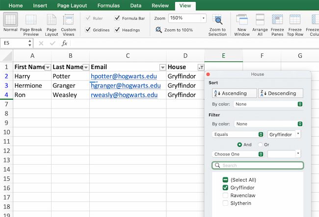
To add a filter, click the Data tab and select «Filter.» Next, click the arrow next to the column headers. This lets you choose whether you want to organize your data in ascending or descending order, as well as which rows you want to show.
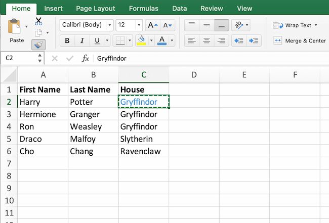
Let’s take a look at the Harry Potter example below. Say you only want to see the students in Gryffindor. By selecting the Gryffindor filter, the other rows disappear.
Pro tip: Start with a filtered view in your original spreadsheet. Then, copy and paste the values to another spreadsheet before you start analyzing.
Sort
Sometimes you’ll have a disorganized list of data. This is typical when you’re exporting lists, like marketing contacts or blog posts. Excel’s sort feature can help you alphabetize any list.
Click on the data in the column you want to sort. Then click on the «Data» tab in your toolbar and look for the «Sort» option on the left.
- If the «A» is on top of the «Z,» you can just click on that button once. Choosing A-Z means the list will sort in alphabetical order.
- If the «Z» is on top of the «A,» click the button twice. Z-A selection means the list will sort in reverse alphabetical order.
Remove Duplicates
Large datasets tend to have duplicate content. For example, you may have a list of different company contacts, but you only want to see the number of companies you have. In situations like this, removing duplicates comes in handy.
To remove duplicates, highlight the row or column where you noticed duplicate data. Then, go to the Data tab, and select «Remove Duplicates» (under Tools). A pop-up will appear so that you can confirm which data you want to keep. Select «Remove Duplicates,» and you’re good to go.
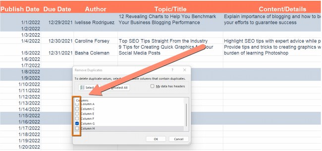
If you want to see an example, this post offers step-by-step instructions for removing duplicates.
You can also use this feature to remove an entire row based on a duplicate column value. So, say you have three rows of information and you only need to see one, you can select the whole dataset and then remove duplicates. The resulting list will have only unique data without any duplicates.
Paste Special
It’s often helpful to change the items in a row of data into a column (or vice versa). It would take a lot of time to copy and paste each individual header.
Not to mention, you may easily fall into one of the biggest, most unfortunate Excel traps — human error. Read here to check out some of the most common Microsoft Excel errors.
Instead of making one of these errors, let Excel do the work for you. Take a look at this example:
To use this function, highlight the column or row you want to transpose. Then, right-click and select «Copy.»
Next, select the cells where you want the first row or column to begin. Right-click on the cell, and then select «Paste Special.»
When the module appears, choose the option to transpose.
Paste Special is a super useful function. In the module, you can also choose between copying formulas, values, formats, or even column widths. This is especially helpful when it comes to copying the results of your pivot table into a chart.
Text to Columns
What if you want to split out information that’s in one cell into two different cells? For example, maybe you want to pull out someone’s company name through their email address. Or you want to separate someone’s full name into a first and last name for your email marketing templates.
Thanks to Microsoft Excel, both are possible. First, highlight the column where you want to split up. Next, go to the Data tab and select «Text to Columns.» A module will appear with more information. First, you need to select either «Delimited» or «Fixed Width.»
- Delimited means you want to break up the column based on characters such as commas, spaces, or tabs.
- Fixed Width means you want to select the exact location in all the columns where you want the split to occur.
Select «Delimited» to separate the full name into first name and last name.
Then, it’s time to choose the delimiters. This could be a tab, semicolon, comma, space, or something else. (For example, «something else» could be the «@» sign used in an email address.) Let’s choose the space for this example. Excel will then show you a preview of what your new columns will look like.
When you’re happy with the preview, press «Next.» This page will allow you to select Advanced Formats if you choose to. When you’re done, click «Finish.»
Format Painter
Excel has a lot of features to make crunching numbers and analyzing your data quick and easy. But if you ever spent some time formatting a spreadsheet, you know it can get a bit tedious.
Don’t waste time repeating the same formatting commands over and over again. Use the format painter to copy formatting from one area of the worksheet to another.
To do this, choose the cell you’d like to replicate. Then, select the format painter option (paintbrush icon) from the top toolbar. When you release the mouse, your cell should show the new format.
Keyboard Shortcuts
Creating reports in Excel is time-consuming enough. How can we spend less time navigating, formatting, and selecting items in our spreadsheet? Glad you asked. There are a ton of Excel shortcuts out there, including some of our favorites listed below.
Create a New Workbook
PC: Ctrl-N | Mac: Command-N
Select Entire Row
PC: Shift-Space | Mac: Shift-Space
Select Entire Column
PC: Ctrl-Space | Mac: Control-Space
Select Rest of Column
PC: Ctrl-Shift-Down/Up | Mac: Command-Shift-Down/Up
Select Rest of Row
PC: Ctrl-Shift-Right/Left | Mac: Command-Shift-Right/Left
Add Hyperlink
PC: Ctrl-K | Mac: Command-K
Open Format Cells Window
PC: Ctrl-1 | Mac: Command-1
Autosum Selected Cells
PC: Alt-= | Mac: Command-Shift-T
Excel Formulas
At this point, you’re getting used to Excel’s interface and flying through quick commands on your spreadsheets.
Now, let’s dig into the core use case for the software: Excel formulas. Excel can help you do simple arithmetic like adding, subtracting, multiplying, or dividing any data.
- To add, use the + sign.
- To subtract, use the — sign.
- To multiply, use the * sign.
- To divide, use the / sign.
- To use exponents, use the ^ sign.
Remember, all formulas in Excel must begin with an equal sign (=). Use parentheses to make sure certain calculations happen first. For example, consider how =10+10*10 is different from =(10+10)*10.
Besides manually typing in simple calculations, you can also refer to Excel’s built-in formulas. Some of the most common include:
- Average: =AVERAGE(cell range)
- Sum: =SUM(cell range)
- Count: =COUNT(cell range)
Also note that series’ of specific cells are separated by a comma (,), while cell ranges are notated with a colon (:). For example, you could use any of these formulas:
- =SUM(4,4)
- =SUM(A4,B4)
- =SUM(A4:B4)
Conditional Formatting
Conditional formatting lets you change a cell’s color based on the information within the cell. For example, say you want to flag a category in your spreadsheet.
To get started, highlight the group of cells you want to use conditional formatting on. Then, choose «Conditional Formatting» from the Home menu. Next, select a logic option from the dropdown. A window will pop up that prompts you to provide more information about your formatting rule. Select «OK» when you’re done, and you should see your results automatically appear.
Note: You can also create your own logic if you want something beyond the dropdown choices.
Dollar Signs
Have you ever seen a dollar sign in an Excel formula? When this symbol is in a formula, it isn’t representing an American dollar. Instead, it makes sure that the exact column and row stay the same even if you copy the same formula in adjacent rows.
You see, a cell reference — when you refer to cell A5 from cell C5, for example — is relative by default.
This means you’re actually referring to a cell that’s five columns to the left (C minus A) and in the same row (5). This is called a relative formula.
When you copy a relative formula from one cell to another, it’ll adjust the values in the formula based on where it’s moved. But sometimes, you want those values to stay the same no matter whether they’re moved around or not. You can do that by making the formula in the cell into what’s called an absolute formula.
To change the relative formula (=A5+C5) into an absolute formula, precede the row and column values with dollar signs, like this: (=$A$5+$C$5).
Combine Cells Using «&»
Databases tend to split out data to make it as exact as possible. For example, instead of having data that shows a person’s full name, a database might have the data as a first name and then a last name in separate columns.
In Excel, you can combine cells with different data into one cell by using the «&» sign in your function. The example below uses this formula: =A2&» «&B2.
Let’s go through the formula together using an example. So, let’s combine first names and last names into full names in a single column.
To do this, put your cursor in the blank cell where you want the full name to appear. Next, highlight one cell that contains a first name, type in an «&» sign, and then highlight a cell with the corresponding last name.
But you’re not finished. If all you type in is =A2&B2, then there will not be a space between the person’s first name and last name. To add that necessary space, use the function =A2&» «&B2. The quotation marks around the space tell Excel to put a space between the first and last name.
To make this true for multiple rows, drag the corner of that first cell downward as shown in the example.
Pivot Tables
Pivot tables reorganize data in a spreadsheet. A pivot table won’t change the data that you have, but it can sum up values and compare information in a way that’s easy to understand.
For example, let’s look at how many people are in each house at Hogwarts.
To create the Pivot Table, go to Insert > Pivot Table. Excel will automatically populate your pivot table, but you can always change the order of the data. Then, you have four options to choose from.
Report Filter
This allows you to only look at certain rows in your dataset.
For example, to create a filter by house, choose only students in Gryffindor.
Column and Row Labels
These could be any headers or rows in the dataset.
Note: Both Row and Column labels can contain data from your columns. For example, you can drag First Name to either the Row or Column label depending on how you want to see the data.
Value
This section allows you to convert data into a number. Instead of just pulling in any numeric value, you can sum, count, average, max, min, count numbers, or do a few other manipulations with your data. By default, when you drag a field to Value, it always does a count.
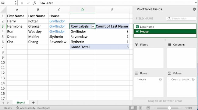
The example above counts the number of students in each house. To recreate this pivot table, go to the pivot table and drag the House column to both the row Labels and the values. This will sum up the number of students associated with each house.
IF Functions
At its most basic level, Excel’s IF function lets you see if a condition you set is true or false for a given value.
If the condition is true, you get one result. If the condition is false, you get another result.
This popular tool is useful for comparisons and finding errors. But if you’re new to Excel you may need a little more information to get the most out of this feature.
Let’s take a look at this function’s syntax:
- =IF(logical_test, value_if_true, [value_if_false])
- With values, this could be: =IF(A2>B2, «Over Budget», «OK»)
In this example, you want to find where you’re overspending. With this IF function, if your spending (what’s in A2) is greater than your budget (what’s in B2), that overspending will be easy to see. Then you can then filter the data so that you see only the line items where you’re going over budget.
The real power of the IF function comes when you string or «nest» multiple IF statements together. This allows you to set multiple conditions, get more specific results, and organize your data into more manageable chunks.
For example, ranges are one way to segment your data for better analysis. For example, you can categorize data into values that are less than 10, 11 to 50, or 51 to 100.
- =IF(B3<11,»10 or less»,IF(B3<51,»11 to 50″,IF(B3<100,»51 to 100″)))
Let’s talk about a few more IF functions.
COUNTIF Function
The power of IF functions goes beyond simple true and false statements. With the COUNTIF function, Excel can count the number of times a word or number appears in any range of cells.
For example, let’s say you want to count the number of times the word «Gryffindor» appears in this data set.
Take a look at the syntax.
- The formula: =COUNTIF(range, criteria)
- The formula with variables from the example below: =COUNTIF(D:D,»Gryffindor»)
In this formula, there are several variables:
Range
The range that you want the formula to cover.
In this one-column example, «D:D» shows that the first and last columns are both D. If you want to look at columns C and D, use «C:D.»
Criteria
Whatever number or piece of text you want Excel to count.
Only use quotation marks if you want the result to be text instead of a number. In this example, «Gryffindor» is the only criteria.
To use this function, type the COUNTIF formula in any cell and press «Enter.» Using the example above, this action will show how many times the word «Gryffindor» appears in the dataset.
SUMIF Function
Ready to make the IF function a bit more complex? Let’s say you want to analyze the number of leads your blog has generated from one author, not the entire team.
With the SUMIFS function, you can add up cells that meet certain criteria. You can add as many different criteria to the formula as you like.
Here’s your formula:
- =SUMIFS(sum_range, criteria_range1, criteria1, [criteria_range2, criteria 2],etc.)
That’s a lot of criteria. Let’s take a look at each part:
Sum_range
The range of cells you’re going to add up.
Criteria_range1
The range that is being searched for your first value.
Criteria1
This is the specific value that determines which cells in Criteria_range1 to add together.
Note: Remember to use quotation marks if you’re searching for text.
In the example below, the SUMIF formula counts the total number of house points from Gryffindor.

If AND/OR
The OR and AND functions round out your IF function choices. These functions check multiple arguments. It returns either TRUE or FALSE depending on if at least one of the arguments is true (this is the OR function), or if all of them are true (this is the AND function).
Lost in a sea of «and’s» and «or’s»? Don’t check out yet. In practice, OR and AND functions will never be used on their own. They need to be nested inside of another IF function. Recall the syntax of a basic IF function:
- =IF(logical_test, value_if_true, [value_if_false])
- Now, let’s fit an OR function inside of the logical_test: =IF(OR(logical1, logical2), value_if_true, [value_if_false])
To put it plainly, this combined formula allows you to return a value if both conditions are true, as opposed to just one. With AND/OR functions, your formulas can be as simple or complex as you want them to be, as long as you understand the basics of the IF function.
VLOOKUP
Have you ever had two sets of data on two different spreadsheets that you want to combine into a single spreadsheet?
For example, say you have a list of names and email addresses in one spreadsheet and a list of email addresses and company names in a different spreadsheet. But you want the names, email addresses, and company names of those people to appear in one spreadsheet.
VLOOKUP is a great go-to formula for this.
Before you use the formula, be sure that you have at least one column that appears identically in both places.
Note: Scour your data sets to make sure the column of data you’re using to combine spreadsheets is exactly the same. This includes removing any extra spaces.
In the example below, Sheet One and Sheet Two are both lists with different information about the same people. The common thread between the two is their email addresses. Let’s combine both datasets so that all the house information from Sheet Two translates over to Sheet One.
Type in the formula: =VLOOKUP(C2,Sheet2!A:B,2,FALSE). This will bring all the house data into Sheet One.
Now that you’ve seen how VLOOKUP works, let’s review the formula.
- The formula: =VLOOKUP(lookup value, table array, column number, [range lookup])
- The formula with variables from the example: =VLOOKUP(C2,Sheet2!A:B,2,FALSE)
In this formula, there are several variables.
Lookup Value
A value that LOOKUP searches for in an array. So, your lookup value is the identical value you have in both spreadsheets.
In the example, the lookup value is the first email address on the list, or cell 2 (C2).
Table Array
Table arrays hold column-oriented or tabular data, like the columns on Sheet Two you’re going to pull your data from.
This table array includes the column of data identical to your lookup value in Sheet One and the column of data you’re trying to copy to Sheet Two.
In the example, «A» means Column A in Sheet Two. The «B» means Column B.
So, the table array is «Sheet2!A:B.»
Column Number
Excel refers to columns as letters and rows as numbers. So, the column number is the selected column for the new data you want to copy.
In the example, this would be the «House» column. «House» is column 2 in the table array.
Note: Your range can be more than two columns. For example, if there are three columns on Sheet Two — Email, Age, and House — and you also want to bring House onto Sheet One, you can still use a VLOOKUP. You just need to change the «2» to a «3» so it pulls back the value in the third column. The formula for this would be: =VLOOKUP(C2:Sheet2!A:C,3,false).]
Range Lookup
This term means that you’re looking for a value within a range of values. You can also use the term «FALSE» to pull only exact value matches.
Note: VLOOKUP will only pull back values to the right of the column containing your identical data on the second sheet. This is why some people prefer to use the INDEX and MATCH functions instead.
INDEX MATCH
Like VLOOKUP, the INDEX and MATCH functions pull data from another dataset into one central location. Here are the main differences:
VLOOKUP is a much simpler formula.
If you’re working with large datasets that need thousands of lookups, the INDEX MATCH function will decrease load time in Excel.
INDEX MATCH formulas work right-to-left.
VLOOKUP formulas only work as a left-to-right lookup. So, if you need to do a lookup that has a column to the right of the results column, you’d have to rearrange those columns to do a VLOOKUP. This can be tedious with large datasets and lead to errors.
Let’s look at an example. Let’s say Sheet One contains a list of names and their Hogwarts email addresses. Sheet Two contains a list of email addresses and each student’s Patronus.
The information that lives in both sheets is the email addresses column. But, the column numbers for email addresses are different on the two sheets. So, you’d use the INDEX MATCH formula instead of VLOOKUP to avoid column-switching errors.
The INDEX MATCH formula is the MATCH formula nested inside the INDEX formula.
- The formula: =INDEX(table array, MATCH formula)
- This becomes: =INDEX(table array, MATCH (lookup_value, lookup_array))
- The formula with variables from the example: =INDEX(Sheet2!A:A,(MATCH(Sheet1!C:C,Sheet2!C:C,0)))
Here are the variables:
Table Array
The range of columns on Sheet Two that contain the new data you want to bring over to Sheet One.
In the example, «A» means Column A, and has the «Patronus» information for each person.
Lookup Value
This Sheet One column has identical values in both spreadsheets.
In the example, this is the «email» column on Sheet One, which is Column C. So, Sheet1!C:C.
Lookup Array
Again, an array is a group of values in rows and columns that you want to search.
In this example, the lookup array is the column in Sheet Two that contains identical values in both spreadsheets. So, the «email» column on Sheet Two, Sheet2!C:C.
Once you have your variables set, type in the INDEX MATCH formula. Add it where you want the combined information to populate.
Data Visualization
Now that you’ve learned formulas and functions, let’s make your analysis visual. With a beautiful graph, your audience will be able to process and remember your data more easily.
Create a Basic Graph
First, decide what type of graph to use. Bar charts and pie charts help you compare categories. Pie charts compare part of a whole and are often best when one of the categories is way larger than the others. Bar charts highlight incremental differences between categories. Finally, line charts can help display trends over time.
This post can help you find the best chart or graph for your presentation.
Next, highlight the data you want to turn into a chart. Then choose «Charts» in the top navigation. You can also use Insert > Chart if you have an older version of Excel. Then you can adjust and resize your chart until it makes the statement you’re hoping for.
Microsoft Excel Can Help Your Business Grow
Excel is a useful tool for any small business. Whether you’re focused on marketing, HR, sales, or service, these Microsoft Excel tips can boost your performance.
Whether you want to improve efficiency or productivity, Excel can help. You can find new trends and organize your data into usable insights. It can make your data analysis easier to understand and your daily tasks easier.
All it takes is a little know-how and some time with the software. So start learning, and get ready to grow.
Editor’s note: This post was originally published in April 2018 and has been updated for comprehensiveness.

Here you will find a detailed tutorial on 100+ Excel Functions & VBA Functions. Each Excel function is covered in detail with Examples and Videos.
Excel Functions – Date and Time
| Excel Function | Description |
|---|---|
| Excel DATE Function |
Excel DATE function can be used when you want to get the date value using the year, month and, day values as the input arguments. It returns a serial number that represents a specific date in Excel. |
| Excel DATEVALUE Function |
Excel DATEVALUE function is best suited for situations when a date is stored as text. This function converts the date from text format to a serial number that Excel recognizes as a date. |
| Excel DAY Function |
Excel DAY function can be used when you want to get the day value (ranging between 1 to 31) from a specified date. It returns a value between 0 and 31 depending on the date used as the input. |
| Excel HOUR Function |
Excel HOUR function can be used when you want to get the HOUR integer value from a specified time value. It returns a value between 0 (12:00 A.M.) and 23 (11:00 P.M.) depending on the time value used as the input |
| Excel MINUTE Function |
Excel MINUTE function can be used when you want to get the MINUTE integer value from a specified time value. It returns a value between 0 and 59 depending on the time value used as the input. |
| Excel NETWORKDAYS Function | Excel NETWORKDAYS function can be used when you want to get the number of working days between two given dates. It does not count the weekends between the specified dates (by default the weekend is Saturday and Sunday). It can also exclude any specified holidays. |
| Excel NETWORKDAYS.INTL Function |
Excel NETWORKDAYS.INTL function can be used when you want to get the number of working days between two given dates. It does not count the weekends and holidays, both of which can be specified by the user. It also enables you to specify the weekend (for example, you can specify Friday and Saturday as the weekend, or only Sunday as the weekend). |
| Excel NOW Function | Excel NOW function can be used to get the current date and time value. |
| Excel SECOND Function |
Excel SECOND function can be used want to get the integer value of the seconds from a specified time value. It returns a value between 0 and 59 depending on the time value used as the input. |
| Excel TODAY Function | Excel TODAY function can be used to get the current date. It returns a serial number that represents the current date. |
| Excel WEEKDAY Function |
Excel WEEKDAY function can be used to get the day of the week as a number for the specified date. It returns a number between 1 and 7 that represents the corresponding day of the week. |
| Excel WORKDAY Function |
Excel WORKDAY function can be used when you want to get the date after a given number of working days. By default, it takes Saturday and Sunday as the weekend |
| Excel WORKDAY.INTL Function |
Excel WORKDAY.INTL function can be used when you want to get the date after a given number of working days. In this function, you can specify the weekend to be days other than Saturday and Sunday. |
| Excel DATEDIF Function |
Excel DATEDIF function can be used when you want to calculate the number of years, months, or days between the two specified dates. A good example would be calculating the age. |
Excel Functions – Logical
| Excel Function | Description |
|---|---|
| Excel AND Function |
Excel AND function can be used when you want to check multiple conditions. It returns TRUE only when all the given conditions are true. |
| Excel FALSE Function |
Excel FALSE function returns the logical value FALSE. It does not take any input arguments. |
| Excel IF Function |
Excel IF Function is best suited for situations where you want to evaluate a condition, and the return a value if it is TRUE and another value if it is FALSE. |
| Excel IFS Function |
Excel IFS Function is best suited for situations where you want to test multiple conditions at once and then return the result based on it. This is helpful as you don’t have to create long nested IF formulas that can get confusing. |
| Excel IFERROR Function | Excel IFERROR function is best-suited to handle formula that evaluates to an error. You can specify a value to show if the formula returns an error. |
| Excel NOT Function |
Excel NOT function can be used when you want to reverse the value of a logical argument (TRUE/FALSE). |
| Excel OR Function | Excel OR function can be used when you want to check multiple conditions. It returns TRUE if any of the given condition is true. |
| Excel TRUE Function |
Excel TRUE function returns the logical value TRUE. It does not take any input arguments. |
Excel Functions – Lookup & Reference
| Excel Function | Description |
|---|---|
| Excel COLUMN Function |
Excel COLUMN function can be used when you want to get the column number of a specified cell. |
| Excel COLUMNS Function |
Excel COLUMNS function can be used when you want to get the number of columns in a specified range or array. It returns a number that represents the total number of columns in the specified range or array. |
| Excel HLOOKUP Function |
Excel HLOOKUP function is best suited for situations when you are looking for a matching data point in a row, and when the matching data point is found, you go down that column and fetch a value from a cell which is specified a number of rows below the top row. |
| Excel INDEX Function |
Excel INDEX function can be used when you have the position (row number and column number) of a value in a table, and you want to fetch that value. This is often use with the MATCH function and is a powerful alternative to the VLOOKUP function. |
| Excel INDIRECT Function |
Excel INDIRECT function can be used when you have the references as text and you want to get the values from those references. It returns the reference specified by the text string. |
| Excel MATCH Function |
Excel MATCH function can be used when you want to get the relative position of a lookup value in a list or an array. It returns a number that represents the position of the lookup value in the array. |
| Excel OFFSET Function |
Excel OFFSET function can be used when you want to get a reference which offsets specified number of rows and columns from the starting point. It returns the reference that OFFSET function points to. |
| Excel ROW Function |
Excel ROW Function function can be used when you want to get the row number of a cell reference. For example, =ROW(B4) would return 4, as it is in the fourth row. |
| Excel ROWS Function |
Excel ROWS Function can be used when you want to get the number of rows in a specified range or array. It returns a number that represents the total number of rows in the specified range or array. |
| Excel VLOOKUP Function |
Excel VLOOKUP function is best suited for situations when you are looking for a matching data point in a column, and when the matching data point is found, you go to the right in that row and fetch a value from a cell which is a specified number of columns to the right. |
| Excel XLOOKUP Function |
Excel XLOOKUP function is a new function for Office 365 users and is an enhanced version of the VLOOKUP/HLOOKUP functions. It can be used to lookup and fetch the value in a dataset, and can replace most of what we do with older lookup formulas. |
| Excel FILTER Function |
Excel FILTER function is a new function for Office 365 users that allows you to quickly filter and extract data based on the given condition (or multiple conditions). |
Excel Functions – Math
| Excel Function | Description |
|---|---|
| Excel INT Function |
Excel INT Function can be used when you want to get the integer portion of a number. |
| Excel MOD Function |
Excel MOD function can be used when you want to get the remainder when one number is divided by another. It returns a numerical value that represents the remainder when one number is divided by another. |
| Excel RAND Function |
Excel RAND function can be used when you want to generate evenly distributed random numbers between 0 and 1. It returns a number between 0 and 1 |
| Excel RANDBETWEEN Function |
Excel RANDBETWEEN function can be used when you want to generate evenly distributed random numbers between a top and bottom range specified by the user. It returns a number between the top and bottom range specified by the user. |
| Excel ROUND Function |
Excel ROUND function can be used when you want to return a number rounded to a specified number of digits. |
| Excel SUM Function | Excel SUM function can be used to add all numbers in a range of cells. |
| Excel SUMIF Function |
Excel SUMIF function can be used when you want to add the values in a range if the specified condition is met. |
| Excel SUMIFS Function |
Excel SUMIFS function can be used when you want to add the values in a range if multiple specified criteria are met. |
| Excel SUMPRODUCT Function |
Excel SUMPRODUCT function can be used when you want to first multiply two or more sets to arrays and then get its sum |
Excel Functions – Statistics
| Excel Function | Description |
|---|---|
| Excel RANK Function |
Excel RANK function can be used when you want to rank a number against a list of numbers. It returns a number that represents the relative rank of the number against the list of numbers. |
| Excel AVERAGE Function |
Excel AVERAGE function can be used when you want to get the average (arithmetic mean) of the specified arguments. |
| Excel AVERAGEIF Function |
Excel AVERAGEIF function can be used when you want to get the average (arithmetic mean) of all the values in a range of cells that meet a given criteria. |
| Excel AVERAGEIFS Function |
Excel AVERAGEIFS function can be used when you want to get the average (arithmetic mean) of all the cells in a range that meets multiple criteria. |
| Excel COUNT Function | Excel COUNT function can be used to count the number of cells that contain numbers. |
| Excel COUNTA Function |
Excel COUNTA function can be used when you want to count all the cells in a range that are not empty. |
| Excel COUNTBLANK Function |
Excel COUNTBALNK function can be used when you have to count all the empty cells in a range. |
| Excel COUNTIF Function |
Excel COUNTIF function can be used when you want to count the number of cells that meet a specified criterion. |
| Excel COUNTIFS Function |
Excel COUNTIFS function can be used when you want to count the number of cells that meet a single or multiple criteria. |
| Excel LARGE Function |
Excel LARGE function can be used to get the Kth largest value from a range of cells or array. For example, you can get the third largest value from a range of cells. |
| Excel MAX Function |
Excel MAX function can be used when you want to get the largest value from a set of values. |
| Excel MIN Function |
Excel MIN function can be used when you want to get the smallest value from a set of values. |
| Excel SMALL Function |
Excel SMALL function can be used to get the Kth smallest value from a range of cells or array. For example, you can get the third smallestvalue from a range of cells. |
Excel Functions – Text Functions
| Excel Function | Description |
|---|---|
| Excel CONCATENATE Function |
Excel CONCATENATE function can be used when you want to join 2 or more characters or strings. It can be used to join text, numbers, cell references, or a combination of these. |
| Excel FIND Function |
Excel FIND function can be used when you want to locate a text string within another text string and find its position. It returns a number that represents the starting position of the string you are finding in another string. It is case-sensitive. |
| Excel LEFT Function | Excel LEFT function can be used to extract text from left of the string. It returns the specified number of characters from the left of the string |
| Excel LEN Function |
Excel LEN function can be used when you want to get the total number of characters in a specified string. This is useful when you want to know the length of a string in a cell. |
| Excel LOWER Function |
Excel LOWER function can be used when you want to convert all uppercase letter in a text string to lowercase. Numbers, special characters, and punctuations are not changed by the LOWER function. |
| Excel MID Function |
Excel MID function can be used to extract a specified number of characters from a string. It returns the sub-string from a string. |
| Excel PROPER Function |
Excel PROPER function can be used when you want to capitalize the first character of every word. Numbers, special characters, and punctuations are not changed by the PROPER function. |
| Excel REPLACE Function |
Excel REPLACE function can be used when you want to replace a part of the text string with another string. It returns a text string where a part of the text has been replaced by the specified string. |
| Excel REPT Function |
Excel REPT function can be used when you want to repeat a specified text a certain number of times. |
| Excel RIGHT Function | The RIGHT function can be used to extract text from the right of the string. It returns the specified number of characters from the right of the string |
| Excel SEARCH Function |
Excel SEARCH function can be used when you want to locate a text string within another text string and find its position. It returns a number that represents the starting position of the string you are finding in another string. It is NOT case-sensitive. |
| Excel SUBSTITUTE Function
|
Excel SUBSTITUTE function can be used when you want to substitute text with new specified text in a string. It returns a text string where an old text has been substituted by the new one. |
| Excel TEXT Function |
Excel TEXT function can be used when you want to convert a number to text format and display it in a specified format. |
| Excel TRIM Function | Excel TRIM function can be used when you want to remove leading, trailing, and double spaces in Excel. |
| Excel UPPER Function | Excel UPPER function can be used when you want to convert all lowercase letters in a text string to uppercase. Numbers, special characters, and punctuations are not changed by the UPPER function. |
Excel Functions – Info
| Excel Function | Description |
|---|---|
| Excel ISBLANK Function
Excel ISERROR Function Excel ISNA Function Excel ISNUMBER Function Excel ISEVEN Function Excel ISODD Function Excel ISLOGICAL Function Excel ISTEXT Function |
Excel IS function returns TRUE when specified condition is TRUE. For example, ISNA would return TRUE if the cell has a #N/A! error. |
Excel Functions – Financial
| Excel Function | Description |
|---|---|
| Excel PMT Function | Excel PMT function helps you calculate the payment you need to make for a loan when you know the total loan amount, interest rate, and the number of constant payments. |
| Excel NPV Function | Excel NPV function allows you to calculate the Net Present Value of all the cashflows when you know the discount rate |
| Excel IRR Function | Excel IRR function allows you to calculate the Internal Rate of Return when you have the cashflows data |
VBA Functions
| Excel Function | Description |
|---|---|
| VBA TRIM Function |
VBA TRIM function allows you to remove the leading and trailing spaces from a text string in Excel. It can be a useful VBA function if you want to quickly clean the data. |
| VBA SPLIT Function |
VBA SPLIT function alllows you to split a text string based on the delimiter. For example, if you want to split text based on a comma or tab or colon, you can do that with the SPLIT function. |
| VBA MsgBox Function |
VBA MsgBox is a function that displays a dialog box that you can use to inform your users by showing a custom message or get some basic inputs (such as Yes/No or OK/Cancel). |
| VBA INSTR Function |
VBA InStr function finds the position of a specified substring within the string and returns the first position of its occurrence. |
| VBA UCase Function |
Excel VBA UCASE function takes a string as the input and converts all the lower case characters into upper case. |
| VBA LCase Function |
Excel VBA LCASE function takes a string as the input and converts all the upper case characters into lower case. |
| VBA DIR Function |
Use VBA DIR function when you want to get the name of the file or a folder, using their path name |
Useful Excel Resources:
- 100+ Excel Interview Questions
- 200+ Excel Keyboard Shortcuts
- Free Excel Templates
- Free Online Excel Training
- Best Excel Books
- Excel Formulas Not Working: Possible Reasons and How to FIX IT!
- 20 Advanced Excel Functions and Formulas (for Excel Pros)
- Formula vs Function in Excel – What’s the Difference?