
Create, load, or edit a query in Excel (Power Query)
Excel for Microsoft 365 Excel 2021 Excel 2019 Excel 2016 Excel 2013 Excel 2010 More…Less
Power Query offers several ways to create and load Power queries into your workbook. You can also set default query load settings in the Query Options window.
Tip To tell if data in a worksheet is shaped by Power Query, select a cell of data, and if the Query context ribbon tab appears, then the data was loaded from Power Query.
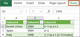
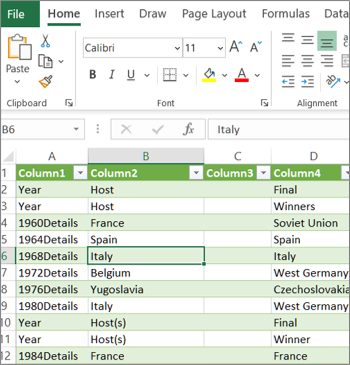
Know which environment you’re in Power Query is well-integrated into the Excel user interface, especially when you import data, work with connections, and edit Pivot Tables, Excel tables, and named ranges. To avoid confusion, it’s important to know which environment you are currently in, Excel or Power Query, at any point in time.
|
The familiar Excel worksheet , ribbon, and grid |
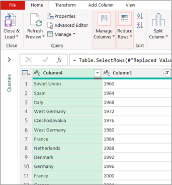
The Power Query Editor ribbon and data preview |
|
|
For example, manipulating data in an Excel worksheet is fundamentally different than Power Query. Furthermore, the connected data that you see in an Excel worksheet, may or may not have Power Query working behind the scenes to shape the data. This only occurs when you load the data to a worksheet or Data Model from Power Query.
Rename worksheet tabs It’s a good idea to rename worksheet tabs in a meaningful way, especially if you have a lot of them. It’s particularly important to clarify the difference between a worksheet of data, and a worksheet loaded from the Power Query Editor. Even if you have only two worksheets, one with an Excel table, called Sheet1, and the other a query created by importing that Excel table, called Table1, it’s easy to get confused. It’s always good practice to change the default names of worksheet tabs to names that make more sense to you. For example, rename Sheet1 to DataTable and Table1 to QueryTable. Now it’s clear which tab has the data and which tab has the query.
You can either create a query from imported data or create a blank query.
Create a query from imported data
This is the most common way to create a query.
-
Import some data. For more information, see Import data from external data sources.
-
Select a cell in the data and then select Query > Edit.
Create a blank query
You may want to just start from scratch. There are two ways to do this.
-
Select Data > Get Data > From Other Sources > Blank Query.
-
Select Data > Get Data > Launch Power Query Editor.
At this point, you can manually add steps and formulas if you know the Power Query M formula language well.
Or you can select Home and then select a command in the New Query group. Do one of the following.
-
Select New Source to add a data source. This command is just like the Data > Get Data command in the Excel ribbon.
-
Select Recent Sources to select from a data source you have been working with. This command is just like the Data > Recent Sources command in the Excel ribbon.
-
Select Enter Data to manually enter data. You might choose this command to try out the Power Query Editor independent of an external data source.
Assuming your query is valid and has no errors, you can load it back to a worksheet or Data Model.
Load a query from the Power Query Editor
In the Power Query Editor, do one of the following:
-
To load to a worksheet, select Home > Close & Load > Close & Load.
-
To load to a Data Model, select Home > Close & Load > Close & Load To.
In the Import Data dialog box, select Add this data to the Data Model.
Tip Sometimes the Load To command is dimmed or disabled. This can occur the first time you create a query in a workbook. If this occurs, select Close & Load, in the new worksheet, select Data > Queries & Connections > Queries tab, right click the query, and then select Load To. Alternatively, on the Power Query Editor ribbon select Query > Load To.
Load a query from the Queries and Connections pane
In Excel, you may want to load a query into another worksheet or Data Model.
-
In Excel, select Data > Queries & Connections, and then select the Queries tab.
-
In the list of queries, locate the query, right click the query, and then select Load To. The Import Data dialog box appears.
-
Decide how you want to import the data, and then select OK. For more information about using this dialog box, select the question mark (?).
There are several ways to edit a query loaded to a worksheet.
Edit a query from data in Excel worksheet
-
To edit a query, locate one previously loaded from the Power Query Editor, select a cell in the data, and then select Query > Edit.
Edit a query from the Queries & Connections pane
You may find the Queries & Connections pane is more convenient to use when you have many queries in one workbook and you want to quickly find one.
-
In Excel, select Data > Queries & Connections, and then select the Queries tab.
-
In the list of queries, locate the query, right click the query, and then select Edit.
Edit a query from the Query Properties dialog box
-
In Excel, select Data > Data & Connections > Queries tab, right click the query and select Properties, select the Definition tab in the Properties dialog box, and then select Edit Query.
Tip If you are in a worksheet with a query, select Data > Properties, select the Definition tab in the Properties dialog box, and then select Edit Query.
A Data Model typically contains several tables arranged in a relationship. You load a query to a Data Model by using the Load To command to display the Import Data dialog box, and then selecting the Add this data to the Data Model check box. For more information about Data Models, see Find out which data sources are used in a workbook data model, Create a Data Model in Excel, and Use multiple tables to create a PivotTable.
-
To open the Data Model, select Power Pivot > Manage.
-
At the bottom of the Power Pivot window, select the worksheet tab of the table you want.
Confirm that the correct table displays. A Data Model can have many tables.
-
Note the name of the table.
-
To close the Power Pivot window, select File > Close. It may take a few seconds to reclaim memory.
-
Select Data > Connections & Properties > Queries tab, right click the query, and then select Edit.
-
When finished making changes in the Power Query Editor, select File > Close & Load.
Result
The query in the worksheet and the table in the Data Model are updated.
If you notice that loading a query to a Data Model takes much longer than loading to a worksheet, check your Power Query steps to see if you are filtering a text column or a List structured column by using a Contains operator. This action causes Excel to enumerate again through the entire data set for each row. Furthermore, Excel can’t effectively use multithreaded execution. As a workaround, try using a different operator such as Equals or Begins With.
Microsoft is aware of this problem and it is under investigation.
You can load a Power Query:
-
To a worksheet. In the Power Query Editor, select Home > Close & Load > Close & Load.
-
To a Data Model. In the Power Query Editor, select Home > Close & Load > Close & Load To.
By default, Power Query loads queries to a new worksheet when loading a single query, and loads multiple queries at the same time to the Data Model. You can change the default behavior for all your workbooks or just the current workbook. When setting these options, Power Query doesn’t change query results in the worksheet or the Data Model data and annotations.
You can also dynamically override the default settings for a query by using the Import dialog box which displays after you select Close & Load To.
Global settings that apply to all your workbooks
-
In the Power Query Editor, select File > Options and settings > Query Options.
-
In the Query Options dialog box, on the left side, under the GLOBAL section, select Data Load.
-
Under the Default Query Load Settings section, do the following:
-
Select Use standard load settings.
-
Select Specify custom default load settings, and then select or clear Load to worksheet or Load to Data Model.
-
Tip At the bottom of the dialog box, you can select Restore Defaults to conveniently return to the default settings.
Workbook settings that only apply to the current workbook
-
In the Query Options dialog box, on the left side, under the CURRENT WORKBOOK section, select Data Load.
-
Do one or more of the following:
-
Under Type Detection, select or clear Detect column types and headers for unstructured sources.
The default behavior is to detect them. Clear this option if you prefer to shape the data yourself.
-
Under Relationships, select or clear Create relationships between tables when adding to the Data Model for the first time.
Before loading to the Data Model, the default behavior is to find existing relationships between tables, such as foreign keys in a relational database and import them with the data. Clear this option if you prefer to do this on your own.
-
Under Relationships, select or clear Update relationships when refreshing queries loaded to the Data Model.
The default behavior is to not update relationships. When refreshing queries already loaded to the Data Model, Power Query finds existing relationships between tables such as foreign keys in a relational database and updates them. This might remove relationships created manually after the data was imported or introduce new relationships. However, if you want to do this, select the option.
-
Under Background Data, select or clear Allow data previews to download in the background.
The default behavior is to download data previews in the background. Clear this option if you can want to see all the data right away.
-
See Also
Power Query for Excel Help
Manage queries in Excel
Need more help?
Want more options?
Explore subscription benefits, browse training courses, learn how to secure your device, and more.
Communities help you ask and answer questions, give feedback, and hear from experts with rich knowledge.
26 Sep ’22 by Antonio Nakić-Alfirević
SQL Query function in Excel
If you’re reading this article you probably know that Google Sheets has a QUERY function that allows you to run SQL-like queries against data in the sheet. This function lets you do all sorts of gymnastics with the data in your sheet, be it filtering, aggregating, or pivoting data.
Being a fully-fledged desktop app, Excel tends to be more feature-rich than Google Sheets. This is especially true in the data analytics department where Excel shines with advanced Excel functions as well as Power Query functionality.
However, Excel doesn’t natively have a QUERY function that you can use in cells on the sheet.
In this blog post, I’m going to show you how to add a QUERY function to Excel and give a few examples of how to use it.
First look
Let’s start by taking a look at the function in action.

The function is pretty straightforward. It accepts the SQL query as the first parameter and returns a table with the results of the query.
The results automatically spill to the necessary amount of space. This spilling behavior relies on the dynamic array functionality that’s available in Excel 365 (but isn’t in earlier versions of Microsoft Excel).
Works with Excel tables
In Google Sheets, the QUERY function references data by address (e.g. “A1:B10”) while columns are referenced by letters (e.g. A, B, C…).
This works but has some drawbacks:
- It makes the query sensitive to the location of the data. If the data is moved or if columns are reordered, the query will break.
- It makes the query difficult to read since it uses range addresses and column letters instead of table and column names (e.g. Employees, DateOfBirth…)
- Adding or removing rows can break the query. For example, if the provided range is “A1:H10” the query will only take into account the first 10 rows. If additional rows are added, the query will not take them into account. You can get around this by omitting the end row number (e.g. “A1:H”), but this means that there must be no other content below the data range.
Excel, on the other hand, allows explicitly defining tables (aka ListObjects) that delineate the areas that hold data. Each Excel table has a name, as do its columns. This makes Excel tables very similar to database tables and makes them easier to work with from SQL.

Full SQL syntax support (SQLite)
Under the hood, the Windy.Query function is powered by SQLite – a small but powerful embedded database engine.
When called, the function passes the query to the built-in SQLite engine which has an adapter that lets it use Excel tables as its data source.
This means that the entire SQLite syntax is available for use in queries. In comparison, in Google Sheets, the query syntax is rather limited. It only supports a single table (no joins) and a very small set of built-in functions.
Examples of use
Since the engine under the hood is SQLite, queries can use all operations available in SQLite, including table joins, temp tables, column table expressions, window functions etc… Let’s go over some examples of how to use these in Excel.
Joining tables
Here’s an example of a simple one-to-many join:

The usual way of doing a simple operation such as this one in Excel would be to use xlookup or PowerQuery, but SQL is now another option. And if we needed anything more complex than a simple join, SQL would quickly shine as the most powerful and convenient option of the three.
Merging table rows (union)
Another way we might want to combine two (or more) tables is to combine their rows. We can do this with a SQL UNION operator.
The tables might have some rows in common. If we want to keep only one instance of such rows we would use the regular UNION operator. If we want to keep both versions of rows that are in common, we would use the UNION ALL operator.

Finding differences between two tables
In the previous example, we had two tables that had some rows in common and some rows not. Let’s assume, for example, that the first table contains last year’s list of employees and the second table is the new list of employees.
If we wanted to find out the differences between the two tables, we could easily do that with a bit of SQL.
All of the rows that are in the first table but not in the second one we will mark as “deleted”. All of the rows that are in the second table but not in the first one we will mark as “added”. Here’s what that SQL query looks like:
select
	id, name, 'deleted'
from
	employees e where not exists (select * from Employees_New en where e.id == en.Id)
union
select
	id, name, 'added'
from
	employees_new en where not exists (select * from Employees e where e.id == en.Id)
And here’s what the result looks like:

Ranking rows
Another useful thing we might want to do is rank rows based on some criteria. For example, suppose we have a table with a list of cities. For each city we have its population and the country it belongs to.
Our task is to find the top 3 cities in each country based on population. Here’s how we might do that in SQL.
-- we use this CTE so we can reference the calculated 'rank_pop' column in the where clause
with cte as (
	select
		city,
		country,
		population,
		-- using the RANK() window function
		RANK() OVER (PARTITION BY country ORDER BY population) as rank_pop
	from
		cities c)
select
	*
from
	cte
where
	-- filtering by the 'rank_pop' column from the CTE
	rank_pop <= 3
order by country, rank_pop

This query is a bit more complex than the previous ones. It uses a common table expression and a window function (the rank function), and showcases the ability to write complex SQL in queries.
Queries can also make use of dozens of built-in SQLite functions. Various specialized extended functions such as RegexReplace, GPSDist (GPS distance between two points) and LevDist (fuzzy text matching) are also available.
Updating tables
OK, this next example is a bit of a hack, but a useful one… The query you supply doesn’t need to be a SELECT query. You can do UPDATE/INSERT/DELETE statements as well, and these will modify the data in the target Excel tables.

This can be a handy way to clean and transform data in your tables in place, without having to export/import the data to an external database (e.g. SQL Server, MySql, Postgres…).
This works because the SQLite engine isn’t copying the data. Rather, it’s using an adapter that lets it access live data in the Excel table.
How does the function see Excel tables?
At first glance, it might seem strange that the query can access your workbook tables. After all, we did not pass them in as parameters, and functions normally only work with parameters that are passed to them.
However, the Windy.Query function is aware of the workbook it’s being called from and it can read data from the workbook’s tables without the need for passing them in as parameters. This makes the function much easier to call especially when working with multiple tables.
Column Headers
Results returned by the Windy.Query function can optionally include headers. This is controlled by the second parameter of the function.

The texts in the column headers are determined by the SQL query itself. You can easily rename result columns by aliasing them in the select list.

Automatically refresh results
By default, the SQL query runs as a one-off operation when you enter the formula but does not refresh if the source tables change. However, if you want the query to refresh whenever one of the source tables changes, you can easily do so by setting the autoRefresh argument to true.

Note that the auto-refresh functionality relies on Excel’s RTD (Real-Time Data) server. The RTD server usually throttles updates so functions don’t overwhelm Excel with frequent updates. The default throttle interval is 2s meaning that the function will not update more than once every 2s. To improve responsiveness, you can lower this value to something like 20ms. The simplest way to do this is through the “Configure” dialog in the QueryStorm runtime’s ribbon.

Passing parameters
When needed, SQL queries can use values from cells as parameters. To use a cell as a parameter in a query, start by giving the cell a name (named range).

Once the cell has a name, you can reference it in the query using the @paramName or $paramName syntax.

If automatic refresh is turned on, results will automatically refresh whenever one of the parameter cells changes its value.

Performance
This is all well and good for small tables, you might think, but how does it handle large data sets? Well, it handles them quite well. The function can read source tables of 100k rows and 10 columns within a few milliseconds and can return this amount of data in a second or two. In addition to this, all columns are automatically indexed so searches and joins are extremely performant as well.
This makes the function perform very well, both from the data throughput standpoint as well as from the computational one.
OK, so is this better than the Google Sheets version of the QUERY function?
Yes, dah. Did you read the previous chapters? 😛
Installing the Windy.Query function
So how do you install this function into your Excel? It’s a simple 2-step process.
Step 1 is to install the QueryStorm Runtime add-in (if you don’t already have it). This is a free, 4MB add-in for Excel that lets you install and use various extensions for Excel. It’s basically an app store for Excel.
Step 2 is to click the “Extensions” button in the “QueryStorm” tab in the Excel ribbon, find the Windy.Query package in the “Online” tab, and install it.

What happens if I share the workbook with a user who doesn’t have the function?
Nothing bad. If the other user doesn’t have the function installed, they will see the last results of the query that were returned on your machine. They just won’t be able to refresh the results.
Advanced SQL query editor
Writing SQL queries in the formula bar can get a bit unwieldy. To make queries easier to write, it’s better to use a proper editor, preferably one that offers syntax highlighting and code completion for SQL and knows about the tables in your workbook.
For this purpose, I recommend using the QueryStorm IDE. This is an advanced IDE that lets you use SQL in Excel. You can write the query in the QueryStorm code editor and then paste the query into the Windy.Query function when you’re happy with it (if needed).

The IDE does more than just allow using SQL in Excel. You can use it to create and share functions and addins for Excel. In fact the QueryStorm IDE was used to create the Windy.Query function itself.
The IDE has a free community version for individuals and small companies, while users in larger companies can make use of the free trial license. For paid licenses, check out the pricing page.
You can read more in this blog post that’s dedicated to the QueryStorm SQL IDE.
Video demonstration
For a video demonstration of the Windy.Query function, take a look the following video:
Knowing your way around Excel formulae is a helpful skill, especially if you work with large datasets and multiple worksheets at once. In another article, we showed you the two basic procedures to transfer data from one Excel worksheet to another automatically as a simple alternative to manual copy/paste. Although the Copy and Paste Link and Worksheet Reference functions can make your life easier, Excel has integrated features that require even less effort.
In this guide, we’ll show you how to use Power Query in Excel to import data from various sources and combine and merge tables according to your preferences, all without having to learn any specific code.
What is Excel Power Query?
Power Query is a Microsoft Excel tool that simplifies the two main tasks of any spreadsheet user: importing and sorting data. Before showing all the applications, let’s briefly explore how they work.
How do Power Queries work in Excel?
Power Queries are commands set up in Excel that can be broken down into the following steps:
- Import or connection: You can connect data stored in the cloud, specific service, or local environment. Moreover, you can connect from multiple sources to combine all of your data in one place.
- Editing or transformation: You can change the data according to your preferences, as these will not affect the original source.
- Automate or load: After completing your query, you can then load it into a worksheet or Data Model and update it regularly, without the need to repeat that same process.
So, is Power Query easy to use? Yes. Power Query doesn’t require knowledge of coding or programming and since 2016, it has become an integrated tool in Excel, so there is no longer a need for third-party installation. Like any automation tool, its most attractive feature is the ability to achieve the same results in half the time.
How to use Excel Power Query?
Before showing how you can use Power Query in Excel, note that it only works in the following Excel versions:
- Power Query for Excel 2010 and 2013: To use it, you need this Microsoft add-in. Unfortunately, there are no add-ins available for macOS and you can only refresh the existing query, but not create a new one or edit.
- Power Query for Excel 2016, 2019, or 365: Depending on the version, Power Query will appear under as “Get Data & Transform” or “Get Data” button. This integrated feature allows you to create and edit queries in Windows and Mac.
This article will show you how to use Power Query for Excel 365 on Mac.
How to import data using Excel Power Query?
Importing your data using Power Query is simple, as Excel provides a great variety of data connections that are accessible from your toolbar. Now that you know what Power Query is and the type of data format it can import, let’s look at how you can import data from an Excel spreadsheet.
How to import data from a single sheet in Excel Power Query?
Imagine that you want to analyze the car sales made by an employee in 2021. Using Power Query, you can import the data without affecting the source file at all.
- 1. Open a new Excel spreadsheet and go to Data > Get Data (Power Query). As explained, there are several options depending on the source type. Here, I will select “Get Data (Power Query)” to import a spreadsheet stored locally.

Excel Power Query — Get Data
- 2. Select “Excel workbook”.

Excel Power Query — Select Data source
- 3. Once you have selected your preferred data source, choose your “Connection settings”. Here, I can select the local file by clicking on “Browse”.

Excel Power Query — Connection settings
- 4. For a quicker search, type the source filename in the search bar. Here, I’ve typed ‘SALES’. Select the file, click “Get Data”, and then the “Next” button located on the bottom right-hand corner of the original window.

Excel Power Query — Select file and Get Data
- 5. You should now be able to see the data preview window. If you are using Windows, then you can transform or edit your data at this point. However, Mac will only allow you to load data and then apply any changes needed.

Excel Power Query — Load data
Once you load the data, Excel automatically saves the query in your system. Every time you want to import or format (for Windows), click the “Refresh” icon in the top-right corner to repeat the steps. This will eliminate repetitive manual work and unnecessary human errors.
How to import data from multiple sheets in Excel Power Query?
As mentioned before, Power Query can import data from multiple files at the same time. This is very useful when you don’t want to import all the data from a larger file, and would like to import specific sheets. Here is how you can get data from multiple sheets.
- 1. Repeat steps 1-3 from the previous section.
- 2. Search for your general folder rather than a specific sheet. Here, I’ll search for my ‘SALES2021’ file. Click on “Get Data” and then “Next” located in the bottom right-hand corner.

Excel Power Query — Get data from Multiple Sheets
- 3. As you can see, you can now select the specific sheets of data you’d like to import. I have selected two sheets corresponding to the sales employees I want to compare. Once selected, click “Load”.

Excel Power Query — Load data from Multiple Sheets
- 4. You should now have a new Excel workbook with the two loaded sheets. Below is an example of how Excel has converted my data into a table, each in a separate tab.

In Windows, Power Query also gives you the option to load to a pivot table, pivot chart or simply create a connection for the query. This last option does not import data, but it’s still a useful way of speeding up any data transformation process.
Now that you know how to load data from a single sheet and multiple sheets, let’s see how to edit the query in Excel.
How to Combine Multiple Excel Files Into One
Discover the most popular methods used to manually or automatically combine multiple Excel spreadsheets and data inputs into one master file
READ MORE

How to edit External Data Range Properties in Excel?
A great way to edit future imports using Power Query is to change the settings for the external data range.
- 1. Go to Data > Properties to edit any of the following elements.

Excel Power Query — External Data Range Properties
Below are summaries of the three most useful properties to consider for future queries:
- Query Definition: Leave the “Save query definition” box ticked and change the name to something that will be easier to remember. Don’t forget that the point of Power Query is to reduce the number of steps in data transformation processes.
- Refresh Control: What’s most important here is the “Refresh data when opening the file” option. If you choose this option, then any change you make to the original file will automatically affect the destination file.
- Data Formatting and Layout: If you select “Insert cells for new data, delete unused cells”, any new rows of data added to your source file will be transferred and formatted to coincide with the rest of your Power Query table, and any unused cells will be deleted.
It’s crucial to understand how Excel can transform your data automatically, to boost productivity. Although the most basic features of Power Query in Excel work in a similar way in Windows and Mac, further automation features may vary to a greater extent.
To avoid version incompatibility and create your own automated spreadsheet workflow regardless of your operating system, check out the benefits of using Layer as an alternative to Excel Power Query.
How to remove a connection in Excel?
If you would like to remove a Power Query connection in Excel, follow the steps below:
- 1. Go to Data > Queries & Connections.

- 2. Click on the query you’d like to delete and select “Remove”.

Excel Power Query — Workbook Queries and Connections
- 3. Excel will prompt you with an alert message to make sure you wish to proceed.

If you do not use a workflow automation tool, Power Query is a great way to not only automate updates, edits, or repetitive tasks but also to track any modifications made to the file.
Want to Boost Your Team’s Productivity and Efficiency?
Transform the way your team collaborates with Confluence, a remote-friendly workspace designed to bring knowledge and collaboration together. Say goodbye to scattered information and disjointed communication, and embrace a platform that empowers your team to accomplish more, together.
Key Features and Benefits:
- Centralized Knowledge: Access your team’s collective wisdom with ease.
- Collaborative Workspace: Foster engagement with flexible project tools.
- Seamless Communication: Connect your entire organization effortlessly.
- Preserve Ideas: Capture insights without losing them in chats or notifications.
- Comprehensive Platform: Manage all content in one organized location.
- Open Teamwork: Empower employees to contribute, share, and grow.
- Superior Integrations: Sync with tools like Slack, Jira, Trello, and more.
Limited-Time Offer: Sign up for Confluence today and claim your forever-free plan, revolutionizing your team’s collaboration experience.
Conclusion
In this article, we have shown you how to use Excel Power Query at a basic level in Excel 2016, 2019, and Office 365 for Mac and Windows. It’s a powerful query tool that can import a variety of data sources in terms of file type and storage systems. In a few simple steps, you can automate your most common repetitive tasks, avoid future manual errors, and increase the efficiency of your business.
If you want to learn more advanced methods to automate your workflow in Excel, read our guide on How To Use Macros in Excel To Automate Tasks.
Written by Puneet for Excel 2010, Excel 2013, Excel 2016, Excel 2019
If you are one of those people who work with data a lot, you can be anyone (Accountant, HR, Data Analyst, etc.), power query can be your power tool.
Let me come straight to the point, Power Query is one of the advanced Excel skills that you need to learn and in this tutorial, you will be exploring power query in detail and will be learning to transform data with it.
Let’s get started.
What is Excel Power Query
Power Query is an Excel add-in that you can use for ETL. That means, you can extract data from different sources, transform it, and then load it to the worksheet. You can say POWER QUERY is a data cleansing machine as it has all the options to transform the data. It is real-time and records all the steps that you perform.
Why Should You Use Power Query (Benefits)?
If you have this question in your mind, here’s my answer for you:
- Different Data Sources: You can load data into a power query editor from different data sources, like, CSV, TXT, JSON, etc.
- Transform Data Easily: Normally you use formulas and pivot tables for data transformations but with POWER QUERY you can do a lot of things just with clicks.
- It’s Real-Time: Write a query once and you can refresh it every time there is a change in data, and it will transform the new data which you have updated.
Let me share an example:
Imagine you have 100 Excel files that have data from 100 cities and now your boss wants you to create a report with all the data from those 100 files. OKAY, if you decide to open each file manually and copy and paste data from those files and you need at least one hour for this.
But with the power query, you can do it in minutes. Feeling excited? Good.
Further in this tutorial, you will learn how to use Power Query with a lot of examples, but first, you need to understand its concept.
The Concept of Power Query
To learn power query, you need to understand its concept that works in 3 steps:
1. Get Data
Power query allows you to get data from different sources like web, CSV, text files, multiple workbooks from a folder, and a lot of other sources where we can store data.
2. Transform Data
After getting data in the power query you have a whole bunch of options that you can use to transform it and clean it. It creates queries for all the steps you perform (in a sequence one step after another).
3. Load Data
From the power query editor, you can load the transformed data to the worksheet, or you can directly create a pivot table or a pivot chart or create a data connection only.
Where is Power Query (How to Install it)?
Below you can see how to install access to the power query in the different versions of Microsoft Excel.
Excel 2007
If you are using Excel 2007, I’m sorry PQ is not available for this version so you need to upgrade to the latest version of Excel (Excel for Office 365, Excel 2019, Excel 2016, Excel 2013, Excel 2010).

Excel 2010 and Excel 2013
For 2010 and 2013, you need to install an add-in separately which you can download from this link and once you install it, you’ll get a new tab in the Excel ribbon, like below:

- First, download the add-in from here (Microsoft’s Official Website).
- Once you have downloaded the file, open it and follow the instructions.
- After that, you’ll automatically get the “Power Query” tab on your Excel ribbon.
If somehow that “POWER QUERY” tab doesn’t appear, there is no need to worry about it. You can add it using the COM Add-ins option.
- Go to File Tab ➜ Options ➜ Add-ins.

- In “Add-In” options, select “COM Add-ins” and click GO.
- After that, tick mark “Microsoft Power Query for Excel”.

- In the end, click OK.
Excel 2016, 2019, Office 365
If you are using Excel 2016, Excel 2019, or you have OFFICE 365 subscription, it’s already there on the Data tab, as a group named “GET & TRANSFORM” (I like this name, do you?).
Excel Mac
If you are using Excel in Mac I’m afraid that there is no power query add-in for it and you can only refresh an existing query but you can’t create a new one and or even edit a query (LINK).

Power Query Editor
Power Query has its own editor where you can get the data, perform all the steps to create queries, and then load it to the worksheet. To open the power query editor, you need to go to the Data Tab and in the Get & Transform ➜ Get Data ➜ Launch Power Query Editor.

Below is the first look at the editor which you will get when you open it.

Now, let’s explore each section in detail:
1. Ribbon
Let’s look at all the available tabs:
- File: From the file tab, you can load the data, discard the editor, and open the query settings.
- Home: In the HOME Tab, you have options to manage the loaded data, like, delete and move columns and rows.
- Transform: This tab has all the options which you need to transform and clean the data, like merge columns, transpose, etc.
- Add Column: Here you have the option to add new columns to the data you have in the power editor.
- View: From this tab, you can make changes to the view for the power query editor and data loaded.
2. Applied Steps
On the right side of the editor, you have a query setting pane which includes the name of the query and all the applied steps in a sequence.

When you right-click on a step you have a list of options that you can perform, like, rename, delete, edit, move up or down, etc. and when you click on a step, the editor will take you to the transformation done on that step.

Look at the below where you have the total five steps applied and when I click on the 4th step it takes me to step four’s transformation where the columns name hasn’t changed.

3. Queries
The queries pane on the left side lists all the queries you have in the workbook right now. It’s basically one place where you can manage all the queries.

When you right-click on a query name you can see all the options that you can use (copy, delete, duplicate, etc.)

You can also create a new query by simply right click on the blank space on the queries pane and then select the option for the data source.
4. Formula Bar
As I said, whenever you apply a step in the editor it generates M code for that step, and you can see that code in the formula bar. You can simply click on the formula bar to edit the code.
Once you learn to use M code you can also create step by writing the code and simply clicking on the “FX” button to enter a custom step.

5. Data Preview
The data preview area looks like an Excel worksheet but there’s a little different than a normal worksheet where you can edit a cell or data directly. When you load data into the editor (we will do it in a while) it shows all the columns with the headers with the columns name and then rows with data.

At the top of each column, you can see the data type of the data in the column. When you load data into the editor the power query applies the right data type (almost every time) to each column automatically.
You can click on the top left button on the column header to change the data type applied to the column. It has a list of all the data types from where you can.

And on the left side of the column header there you have the filter button which you can use to filter values from the column. Note: When you filter values from a column, the power query takes it as one step and lists it in the applied steps.

If you right-click on the header of the column you can see that there is a menu that includes a list of the options which you can use to transform the data and use any of the options and PQ stores it as a step in the applied steps.

Data Sources for Power Query
The best part of the power query is you have the option to get data from multiple sources and transform that data and then load it into the worksheet. When you click on the Get Data in the GET & TRANSFORM you can see the complete list of data sources that you can get data load into the editor.

Now let’s look at some of the data sources:
- From Table/Range: With this option, you can load data into the power query editor directly from the active worksheet.
- From Workbook: From a different workbook that you have on your computer. You just need to locate that file using an open dialog box and it will get data from that file automatically.
- From Text/CSV: Get data from a text file or a comma-separated file and then you can load it into the worksheet.
- From Folder: It takes all the files from the folder and load data from them into the power query editor. (See this: Combine Excel Files from a Folder).
- From Web: With this option, you get data from a web address, imagine you have a File that is stored on the web or you have a web page from where you need to get the data.
How to Load Data into Power Query Editor
Now let’s learn to load data into the power query editor. Here you have a list of student names and their scores (LINK).

You will be loading data directly from the worksheet, so you need to open the file first and then follow the below steps:
- First, apply an Excel table to the data (Even if you don’t do it Excel will do it for you before loading data into PQ editor).
- Now, select a cell from the table and click on the “From Table/Range” (Data Tab Get & Transform).

- Once you click on the button, Excel confirms the range of data to apply an Excel table to it.

- At this point, you have the data into the power query editor, and it looks something like below.

- Here you can see:
- In the Formula bar, PQ has generated the M code for the table you have just loaded into the editor.
- On the left side of the editor, you have the queries pane where you have the list of the queries.
- On the right side, in the query settings, you have the section called “Applied Steps” where you have all the steps listed. Note: You must be thinking that you haven’t performed any “Changed Type” but there’s a step called “Changed Type” is there. Let me tell you the SMARTNESS of POWER QUERY when you load data into the editor it checks and applies the correct data types for all the columns automatically.

Power Query Examples (Tips and Tricks)
You can learn to perform some of the basic tasks which you normally do with functional formulas in Excel, but with power query, you can do it with a few clicks:
1. Replace Values
You have a list of values, and you want to replace a value or some values with something else. Well, with the help of the power query you can create a query and replaces those values, in no time.
In the below list, you need to replace my name “Puneet” with “Punit”.

- First, edit the list in the power query editor.
- After that, in the power query editor, go to “Transform Tab” and click “Replace Values”.

- Now, in “Value to Find”, enter “Puneet” and in “Replace With” enter “Punit” and after that, click OK.

- Once you click OK all the values get replaced with the new values and now, click on “Close and Load” to load data in the worksheet.

2. Sort Data
Just like normal sorting, you can sort data by using power query and I’m using the same name list which you have used in the above example.
- First, load data in the power query editor.
- In the Home tab, you have two sorting buttons (Ascending and Descending).
- Click on any of these buttons to sort.

3. Remove Columns
Let’s say you got data from somewhere and you need to delete some columns from it. The thing is, you have to delete those columns every time you add new data, right? But, power query can take care of this.
- Select the column or multiple columns that you want to delete.

- Now, right-click and select “Remove”.

Quick Tip: There’s also an option to “Remove Other Columns” where you can delete all the unselected columns.
4. Split Column
Just like the text to column option, you have “Split Column” in power query. Let me tell you how it works.
- Select the column and go to the Home Tab ➜ Transform ➜ Split Column ➜ By Delimiter.

- Select the custom from the drop-down and enter “-” into it.
- Now, here you have three different options to split a column.
- Left-most Delimiter
- Right-most Delimiter
- Each occurrence of the delimiter

If you have only one delimiter in a cell, all three will work in the same way, but if you have more than one delimiter then you have to choose accordingly.

5. Rename a Column
You can simply rename a column by right click and then click on the “Rename”.

Quick Tip: Let say you have a query for renaming a column and someone else rename it by mistake. You can restore that name just with a click.
6. Duplicate Column
In Power Query, there is a simple option to create a duplicate column. All you need to do is right-click on the column for which you want to create a duplicate column and then click on “Duplicate Column”.

7. Transpose Column or Row
In the power query, transposing is a cup of cake. Yes, just one click.
- Once you load data into the power query editor, you just need to select the column(s) or row(s).
- Go to Transform Tab ➜ Table ➜ Transpose.

8. Replace/Remove Errors
Normally for replacing or removing errors in Excel you can use find and replace option or a VBA code. But in power query, it’s a whole lot easier. Look at the below column where you have some errors and you can remove as well as replace them.

When you right-click on the column, you’ll have both of the options.
- Replace Errors
- Remove Errors

9. Change Data Type
You have data in a column but it’s not in the right format. So, every time you need to change its format.

- First, edit data into the power query editor.
- After that, select the column and go to the Transform Tab.
- Now, from data type select the “Date” as a type.
10. Add Column from Examples
In the power query, there is an option to add a sample column which is not actually a sample related to the current column.
Let me give you an example:
Imagine you need day names from a date column. Instead of using a formula or any other option, you can use, you can use the “Add Column from Examples”.
Here’s how to do this:
- Right-click on a column and click on “Add Column from Examples”.

- Here you’ll get a blank column. Click on the first cell of the column to get the list of values you can insert.

- Select “Day of Week Name from Date” and click OK.

Boom! your new column is here.

11. Change Case
You have the following options for changing the case of text in power query.
- Lower Case
- Upper Case
- Capitalize Each Word
You can do it by right click on a column and select any of the above three options. Or, go to the Transform Tab ➜ Text Column ➜ Format.

12. Trim and Clean
To clear data or delete unwanted spaces you can use TRIM and CLEAN options in power query. Steps are simple:
- Right-click on a column or select all the columns if you have multiple columns.
- Go to Transform Tab ➜ Text Column ➜ Format.
- TRIM: To remove trailing and leading whitespaces from a cell.
- CLEAN: To remove non-printable characters from a cell.

13. Add Prefix/Suffix
If you are a formula savvy, then I’m sure you agree with me that extracting text or number from a cell requires to combine different functions. But power query has solved a lot of these things in a good way. You have seven ways to extract values from a cell.

15. Only Date or Time
It happens a lot of times that you have date and time, both in a single cell, but needs one of them.

- Select the column where you have the date and time combined.
- If you want:
- Date: Right Click ➜ Transform ➜ Date Only.
- Time: Right Click ➜ Transform ➜ Time Only.


16. Combine Date and Time
Now you know how to separate date and time. But the next you need to know how to combine them.

- First, select the date column and click on the “Date Only” option.
- After that, select both columns (Date and Time) and go to the transform tab and from the “Date and Time Column” Group go to Date and click “Combine Date and Time”.

17. Rounding Numbers
Here are the following options which you have for rounding numbers.
- Round Down: To round down a number.
- Round Up: To round up a number.
- Round: You can choose up to how my decimals you can round.

Here are the steps:
- Select the column and right-click ➜ Transform ➜ Round.
- Round Down: To round down a number.
- Round Up: To round up a number.
- Round: You can choose up to how my decimals you can round.
Note: When you select the “#3 Round” option you need to enter the number of decimals to round.
18. Calculations
There are options that you can use to perform calculations (a lot of). You can find all these options on the Transform Tab (in Number Column group).
- Basic
- Statistics
- Scientific
- Trigonometry
- Rounding
- Information

To perform any of this calculation you need to select the column and then the option.
19. Group by
Let’s say you have a large data set and you want to create a summary table. Here’s what you need to do:

- In the Transform tab, click on the ‘Group by“ button and you’ll get a dialog box.

- Now, from this dialog box select the column with which you want to group and after that, add a name, select the operation, and the column where you have values.

- In the end, click OK.

Note: There are also some advanced options in the “Group by” option which you can use to create a multi-level group table.
20. Remove Negative Values
In one of my blog posts, I have listed seven methods to remove the negative signs and the power query is one of them. Just right click on a column and go to transform option and then click on “Absolute value”.

This instantly removes all the negative signs from the values.
More Examples
- How to Unpivot Data in Excel using Power Query
- How to Perform VLOOKUP in Power Query
- How to Merge [Combine] Multiple Excel FILES into ONE WORKBOOK
How to Load Data Back to the Worksheet
Once you transform your data, you can load it to the worksheet and use it for further analysis. On the home tab there is a button called “Close and Load” when you click on it you get a drop-down which has options further:
- Close and Load
- Close and Load To

- Once you click on the button, it will show the following options:

- Select how you want to view this data in your worksheet.
- Table
- Pivot Table Report:
- Pivot Chart
- Only Create Connection
- Where do you want to put the Data?
- Existing Worksheet
- New Worksheet.
- Add this data to the Data Model.
- Just select the table option and new worksheet and don’t tick mark the data model and click OK.

- The moment you click OK, it adds a new worksheet with the data.

More Examples to Learn
Auto Refresh a Query
From all the examples that I have mentioned here, this one is the most important. When you create a query, you can make it auto-refresh (you can set a timer).
And here are the steps:
- On the Data tab, click on “Queries & Connections” and you’ll get the Queries and Connection pane on the right side of the window.

- Now, right-click on the query and tick mark “Refresh every” and enter the minutes.

How to use a Formula and a Function in Power Query
Just like you can use functions and formulas in Excel worksheet, the power query has its own list of functions that you can use. The basics of function and formulas in power query are the same as Excel’s worksheet functions.
In PQ, you need to add a new custom column to add a function or a formula.
Let’s take an example: In the below data (already in the PQ editor) you have the first name and last name (DOWNLOAD LINK).

Imagine you need to merge both names and create a column for the full name. In this case, you can enter a simple formula to concatenate names from both columns.
- First, go to the Add Column tab and click on the “Custom Column”.

- Now in the custom column dialog box, enter the name of the new column “Full Name” or anything you want to name the new column.

- The custom column formula is the place where you need to enter the formula. So enter the below formula in it:
[First Name]&" "&[Last Name]

- When you enter a formula in the “custom column formula”, PQ verify the formula that you have entered and shows a message “No syntax error have been detected” and if there’s an error it will show an error message based on the type of the error.
- Once you enter the formula and that formula doesn’t have any errors in it, simply press OK.
- Now you have a new column at the end of the data which has values from two columns (first name and the last name).

How to use a Function in Power Query
In the same way, you can also use a function while adding a custom column and Power Query has a huge list of functions that you can use.
Let’s understand how to use a function with an easy and simple example. I’m continuing the above example where we have added a new column by combining the first name and last name.

But now, you need to convert that full name text which you have in that column into the upper case. The function which you can use is “Text.Upper”. As the name suggests, it converts a text to an upper-case text.
- First, go to the add column tab and click on the custom column.

- Now in the custom column dialog box, enter the column name and below formula in the custom column formula box:
Text.Upper([Full Name])

- And when you click OK it creates a new column with all the names in the uppercase.
- The next thing is to delete the old column and rename the new column. So right-click on the first column and select remove.

- In the end, rename the new column his “Full Name”.
There are a total of 700 functions that you can use in power query while adding a new column and here is the complete list provided by Microsoft for these functions, do check them out.
How to Edit a Query in PQ
If you want to make some changes in the query which is already in your workbook you can simply edit it and then make those changes. On the Data tab, there’s a button named Queries and Connections.

When you click on this button, it opens a pane on the right side that lists all the queries that you have in the current workbook.

You can right-click on the query name and select edit and you will get it in the power query editor to edit.

When you edit a query, you can see that all the steps which you have performed earlier are listed in the “Applied Steps” that you can also edit or you can perform new steps.

And once you are done with your changes you can simply click on the “Close & Load” button.
Export and Import Connections
If you have a connection which you have used for a query and now you want to share that connection with someone else, you can export that connection as an odc file.
On the query table, there’s a button called “Export Connection” and when you click on it, it allows you to save that query’s connection in your system.

And if you want to import a connection that is shared by someone else, you can simply go to the Data tab and in the Get & Transform click on the existing connections.
And then click on the “Browse for More” button from where you can locate the connection file which has been shared with you and import it to your workbook.

Power Query Language (M Code)
As I mentioned earlier that for every step you performed in power query it generates a code (at the backend) which is called M Code. On the Home tab, there is a button called “Advanced Editor” which you can use to see the code.

And when you click on the advanced editor it will show you the code editor and that code looks something like below:

M is a case sensitive language and like all the other languages it uses variables and expressions. The basic structure of code looks like below where the code starts with the LET expression.

In this code, we have two variables and the values defined to them. In the end, to get the value, IN expression has been used. Now when you click OK it will return the value assigned to the variable “Variablename” in the result.

Check out this resource to learn more about Power Query Language.
In the End
What is Excel Power Query?
Power Query is a data transforming engine which you can use to get data from multiple sources, clean and transform that data and then use it further in the analysis.
You can’t afford to avoid the POWER QUERY. If you think like this, a lot of things which we do with Excel functions or VBA codes can be automated using it, and I’m sure this tutorial inspires you to use it more and more.
But now you need to tell me one thing. Which thing do you like most about the POWER QUERY?
You must check out these tutorials
- Create a Pivot Table from Multiple Files
What is Power Query in Excel?
Power Query is an excel tool used to import data from different sources, transform (change) it as required, and return a refined dataset in the workbook. Every change made to the data is recorded and saved as a step. In future, whenever the data source is updated, the same changes are performed automatically with the click of the “refresh” button.
For example, an organization has 180 files containing the purchases made in the last 15 years. To consolidate and analyze these numbers, either of the following steps can be performed:
- Open the different files and copy-paste the entire data in one worksheet. Apply the various functions of Excel to convert the data into meaningful reports.
- Use Power Query to import data from the different files. Set up a query which consists of making step-by-step changes to the data. Load the transformed data in a worksheet to create reports.
If the organization follows the pointer “a,” it will have to perform a lot of manual work. These tasks are often tedious and repetitive. However, if pointer “b” is followed, the transformations are performed automatically every time data is updated. This saves a lot of time and speeds up the process of consolidating excel dataConsolidate is an inbuilt function in excel which is used to consolidate data from different workbooks which are opened at the same time. It allows to select multiple data from different workbooks and consolidate it in a final workbook.read more.
Power Query in excel performs the extract, transform, and load operations (ETL) on a dataset. All transformations (steps or changes) applied to the data are collectively known as a query. By performing these transformations, the data is said to be shaped.
The major advantage of Power Query in excel is that it is a fast and efficient way of working on large datasets. Besides, it is reusable as the same query can be used again on a new dataset. Moreover, with just a few clicks, one can have access to cleansed and sorted data.
Power Query can be installed as an add-in in ExcelAn add-in is an extension that adds more features and options to the existing Microsoft Excel.read more 2010 and 2013. In Excel 2016 and the subsequent versions, Power Query is a built-in excel feature. It can be accessed from the “get data” drop-down (in the “get and transform data” group) of the Data tab of Excel.
Table of contents
- What is Power Query in Excel?
- Using Power Query in Excel
- Example of Power Query in Excel
- The Key Points Related to Excel Power Query
- Frequently Asked Questions
- Recommended Articles
Using Power Query in Excel
To use Power Query in Excel, the following steps need to be performed:
- Import data: Import data from the different sources. The data source can be a text file, Excel workbook, web, pdf, and so on. With Power Query, one can work with data from any source having any size and shape.
- Transform data: Change, sort and shape data as per the requirements. For instance, one can delete or insert a row and/or column, replace a missing value, delete a duplicate entry, filter a column, and so on. These changes are recorded as a query in the sequence in which they are applied to the data.
- Consolidate data: Consolidate or combine the data from the different sources. Once integrated, a consolidated database can be generated. The merging and appending of queries are carried out at this stage.
- Load data: Load the data on a worksheet once it has been transformed and consolidated. Loading the data helps return an output in the workbook. The output can be in the form of a table, pivot chartIn Excel, a pivot chart is a built-in feature that allows you to summarize selected rows and columns of data in a spreadsheet. It is a visual representation of a pivot table that helps in the summarization and analysis of datasets, patterns, and trends.read more or a pivot tableA Pivot Table is an Excel tool that allows you to extract data in a preferred format (dashboard/reports) from large data sets contained within a worksheet. It can summarize, sort, group, and reorganize data, as well as execute other complex calculations on it.read more. Prior to loading, one can preview the data to ensure it is on the right track.
Note: Each step performed (in pointer 2) is recorded and written in a code of M language.
Example of Power Query in Excel
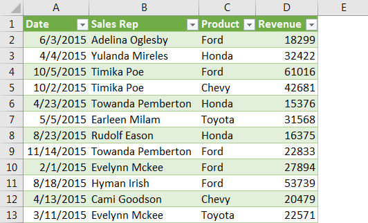
The following image shows two Excel files (“data” and “salesdat”) and two text files (“year 2015 data” and “year 2016 data”). We want to perform the following tasks:
- Import all these files (Excel and text files) to the Power Query editor.
- Combine the data of the two text files. Extract this data as a single table and load it to an Excel worksheet.

The steps to perform the given tasks are listed as follows:
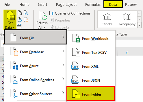
Step 1: To import data, click the drop-down of “get data” (in the “get and transform data” group) from the Data tab of Excel.
Open the options of “from file.” Select “from folder,” as shown in the following image.
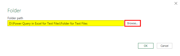
Step 2: Click “browse” and look for the folder containing the text files (shown in the first image of this example). Select the correct path of the folder and click “Ok.”
Step 3: A dialog box opens containing the list of files in the selected folder. The same is shown in the following image.
The column headers of this box are “content,” “name,” “extension,” “date accessed,” “date modified,” “date created,” “attributes,” and “folder path.”
At the bottom of this box, the following options are displayed:
- Combine: This combines all the files of the folder. In other words, the user is not given an option to select the files to be combined. The combine drop-down shows the following options:
- Combine and transform data–This helps consolidate all files with a query. Then, it opens the “power query editor” window.
- Combine and load–This helps create a query and load the data to the worksheet.
- Combine and load to–This opens the “import data” window after a query has been created.
- Load: This displays the following options:
- Load–This loads the data as tables in the worksheet.
- Load to–This opens the “import data” window, which shows more loading options.
- Transform data: This helps create a query and open the “power query editor.” Moreover, it allows choosing the files to be combined. So, one can combine the files having the same extension.
Since only the text files (with extension “.txt”) are to be combined, click “transform data.”
Note: Use “combine” when the folder contains only those files that are to be combined. Use “transform data” when the files to be combined are to be chosen after filtering.

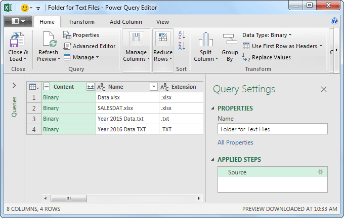
Step 4: The “power query editor” window opens, as shown in the following image. The Excel and text files have been imported to this window.
On the right side, the “query settings” pane is displayed, which consists of “properties” and “applied steps.” Connection with the source folder is the only applied step at present.
Further, there are three columns named “content,” “name,” and “extension” on the left side. The extensions are shown (in the column “extension”) in both lowercase and uppercase.
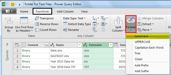
Step 5: Convert all the entries of the column “extension” to lowercase. This is being done because we need to filter the text extensions in the subsequent step (step 6).
For changing the case, select the column “extension” and click the “format” drop-down. Select “lowercase,” as shown in the following image.
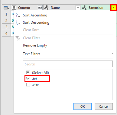
Step 6: Once all the entries of the column “extension” are displayed in lowercase, apply the filters. For this, click the drop-down arrow of the column “extension.” The options of this menu are displayed in the following image.
Since the data of only the text files are to be extracted, select the checkbox of “.txt” and click “Ok.”
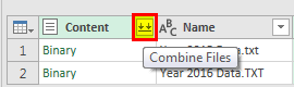
Step 7: To combine the data of the two text files, click the icon displaying near the header “content.” The same is shown within a red box in the following image.
Note: Prior to combining files, ensure that they all have the same extension and structure.
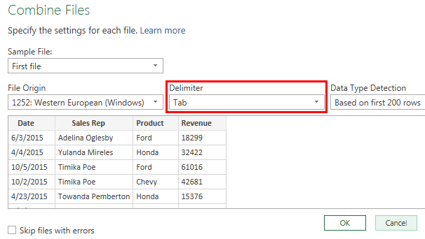
Step 8: A dialog box captioned “combine files” opens, as shown in the following image. Select “tab” as the “delimiter.” This is because a tab separates the entries of the text files.
In “data type detection,” select “based on first 200 rows.” This implies that the data type detection needs to be done on the first 200 rows of the dataset.
One can preview the data of the combined text files on the left side of the “combine files” window. If the preview is fine, click “Ok.”
Note: By default, the first file of the list is used as the sample file. However, one can select a different file as the sample file. For this, use the drop-down menu under “sample file”.
Step 9: The “power query editor” window opens. It shows the data of the combined text files as a single table.
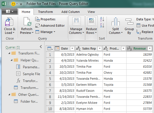
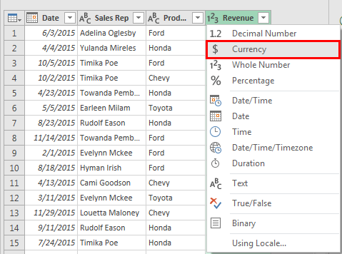
Step 10: Add transformations to the extracted dataset. Change the data type of the “revenue” column to “currency.” For this, click the drop-down near the header “revenue” and select “currency.”
The same is shown in the following image.
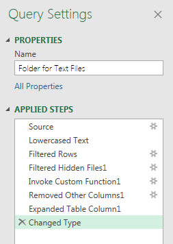
Step 11: The number of applied steps has increased, as shown in the following image.
Note: One can click on any of the “applied steps” to see how data appeared after applying the specific step.
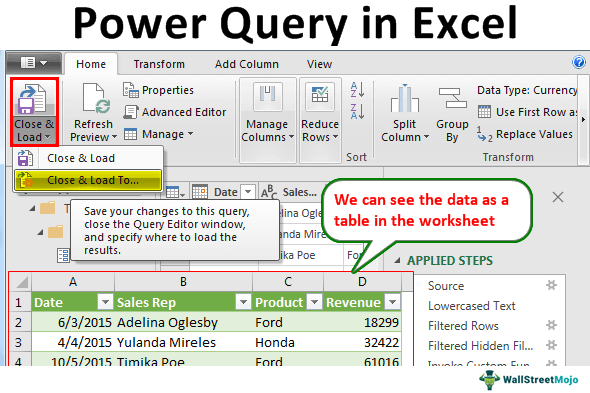
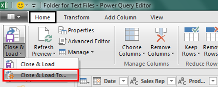
Step 12: Once the transformations to the data are complete, load the combined dataset to an Excel worksheet. For this, click the drop-down of “close and load” (in the “close” group) from the Home tab of the “power query editor” window.
Select “close and load to,” as shown in the following image.
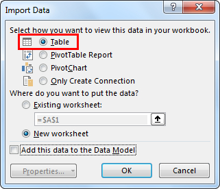
Step 13: The “import data” window opens, as shown in the following image. Select the kind of output required in the worksheet.
Since we want the output in the form of a table, select “table” and click “Ok.”
Note: One can create just a connection with the data by selecting the option “only create connection.” When a connection is created, no output is returned in the workbook. However, the query and the steps applied are saved. This query can be used in other queries.
Step 14: The combined data of the two text files (shown in the first image of this example) appears as a table on the worksheet. Hence, the text files of the D drive have been imported, consolidated, transformed, and loaded in Excel.
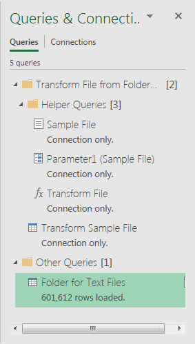
Step 15: One can view the list of workbook queries under the “queries and connections” pane. This pane can be used for navigating, editing, merging, duplicating, appending, and deleting queries.
The following image shows that 601,612 rows have been loaded by Power Query in excel. Hence, by using Power Query, a transformed output has been obtained within a short span of time.
Note 1: One can revise (modify) an existing query with the help of the “edit” option. By revising a query, the steps applied to the data can be edited, deleted or reordered.
Note 2: One can refresh a query when new data is imported. As a query is refreshed, the associated charts, tables, and other data forms are automatically updated.
The important points related to the usage of Power Query are listed as follows:
- Excel Power Query does not make any changes to the original (source) data file. It simply records the transformations made to the dataset. Then, it returns the refined dataset in the workbook.
- Power Query is case-sensitive. This implies that it distinguishes between the lowercase and uppercase versions of the same text.
- Power Query imports temporary files as well. So, such files must be excluded before the consolidation of data. One can filter the “extension” column to exclude the temporary files.
Note: The names of the temporary files begin with the tilde symbol (~). They have the “.tmp” or “.temp” extension.
Frequently Asked Questions
1. What is Power Query? Where and in which versions of Excel can it be found?
Power Query is an excel tool which helps in importing data from different sources, transforming it, and producing a consolidated output. The data sources can be varied like text file, workbook, XML, JSON, web, etc. The output is returned in an Excel workbook.
The purpose of using Power Query in excel is to obtain cleansed data which is suitable for analysis.
In Excel 2016 and the subsequent versions, Power Query can be accessed from the “get data” drop-down (in the “get and transform data” group) of the Data tab of Excel. In Excel 2010 and 2013, Power Query needs to be installed as an add-in. For the versions prior to Excel 2010, Power Query is not available.
2. How to edit an already existing query in Power Query in excel?
In Power Query, an already existing query can be edited as follows:
a. From the Data tab of Excel, click “queries and connections” (in the “queries and connections” group).
b. The “queries and connections” pane opens on the right side of the workbook. This pane shows all the queries of the current workbook.
c. Select the name of the query to be edited. Right-click and select “edit.”
d. The “power query editor” window opens. Either edit the “applied steps” or perform new steps.
e. Once the transformations are complete, click the “close and load” button (in the “close” group) from the Home tab of Excel.
The query is edited, saved, and updated. The dataset in the worksheet is also updated.
3. Are Power Query and Power BI the same? State the major differences between these two tools.
Power Query and Power BI are two different tools. However, Power BI desktop contains Power Query. The major differences between Power Query and Power BI are listed as follows:
a. Power Query sorts and refines the large datasets in order to facilitate data analysis. In contrast, Power BI is a business intelligence tool that helps visualize the data uploaded from multiple sources. These visualizations are presented in the form of reports and dashboards.
b. Power Query reshapes data by allowing one to perform actions on it. This cleaned data is then visualized with Power BI. Power BI also allows sharing of this visualized data. So, Excel Power Query is used before using Power BI.
c. Power Query uses the M (Data Mash-up) language, while Power BI uses M and DAX (Data Analysis Expressions) languages.
Note: Power BI desktop is the desktop version of Power BI, which can be downloaded for free from the Microsoft website.
Recommended Articles
This has been a guide to Power Query in Excel. Here we learn how to use Power Query to manage our data in Excel with the help of step-by-step examples. You can learn more about Excel from the following articles-
- Power BI Query Editor
- Power View in Excel
- Data Model in Excel