
The IF function allows you to make a logical comparison between a value and what you expect by testing for a condition and returning a result if that condition is True or False.
-
=IF(Something is True, then do something, otherwise do something else)
But what if you need to test multiple conditions, where let’s say all conditions need to be True or False (AND), or only one condition needs to be True or False (OR), or if you want to check if a condition does NOT meet your criteria? All 3 functions can be used on their own, but it’s much more common to see them paired with IF functions.
Use the IF function along with AND, OR and NOT to perform multiple evaluations if conditions are True or False.
Syntax
-
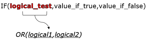
IF(AND()) — IF(AND(logical1, [logical2], …), value_if_true, [value_if_false]))
-
IF(OR()) — IF(OR(logical1, [logical2], …), value_if_true, [value_if_false]))
-
IF(NOT()) — IF(NOT(logical1), value_if_true, [value_if_false]))
|
Argument name |
Description |
|
|
logical_test (required) |
The condition you want to test. |
|
|
value_if_true (required) |
The value that you want returned if the result of logical_test is TRUE. |
|
|
value_if_false (optional) |
The value that you want returned if the result of logical_test is FALSE. |
|
Here are overviews of how to structure AND, OR and NOT functions individually. When you combine each one of them with an IF statement, they read like this:
-
AND – =IF(AND(Something is True, Something else is True), Value if True, Value if False)
-
OR – =IF(OR(Something is True, Something else is True), Value if True, Value if False)
-
NOT – =IF(NOT(Something is True), Value if True, Value if False)
Examples
Following are examples of some common nested IF(AND()), IF(OR()) and IF(NOT()) statements. The AND and OR functions can support up to 255 individual conditions, but it’s not good practice to use more than a few because complex, nested formulas can get very difficult to build, test and maintain. The NOT function only takes one condition.

Here are the formulas spelled out according to their logic:
|
Formula |
Description |
|---|---|
|
=IF(AND(A2>0,B2<100),TRUE, FALSE) |
IF A2 (25) is greater than 0, AND B2 (75) is less than 100, then return TRUE, otherwise return FALSE. In this case both conditions are true, so TRUE is returned. |
|
=IF(AND(A3=»Red»,B3=»Green»),TRUE,FALSE) |
If A3 (“Blue”) = “Red”, AND B3 (“Green”) equals “Green” then return TRUE, otherwise return FALSE. In this case only the first condition is true, so FALSE is returned. |
|
=IF(OR(A4>0,B4<50),TRUE, FALSE) |
IF A4 (25) is greater than 0, OR B4 (75) is less than 50, then return TRUE, otherwise return FALSE. In this case, only the first condition is TRUE, but since OR only requires one argument to be true the formula returns TRUE. |
|
=IF(OR(A5=»Red»,B5=»Green»),TRUE,FALSE) |
IF A5 (“Blue”) equals “Red”, OR B5 (“Green”) equals “Green” then return TRUE, otherwise return FALSE. In this case, the second argument is True, so the formula returns TRUE. |
|
=IF(NOT(A6>50),TRUE,FALSE) |
IF A6 (25) is NOT greater than 50, then return TRUE, otherwise return FALSE. In this case 25 is not greater than 50, so the formula returns TRUE. |
|
=IF(NOT(A7=»Red»),TRUE,FALSE) |
IF A7 (“Blue”) is NOT equal to “Red”, then return TRUE, otherwise return FALSE. |
Note that all of the examples have a closing parenthesis after their respective conditions are entered. The remaining True/False arguments are then left as part of the outer IF statement. You can also substitute Text or Numeric values for the TRUE/FALSE values to be returned in the examples.
Here are some examples of using AND, OR and NOT to evaluate dates.

Here are the formulas spelled out according to their logic:
|
Formula |
Description |
|---|---|
|
=IF(A2>B2,TRUE,FALSE) |
IF A2 is greater than B2, return TRUE, otherwise return FALSE. 03/12/14 is greater than 01/01/14, so the formula returns TRUE. |
|
=IF(AND(A3>B2,A3<C2),TRUE,FALSE) |
IF A3 is greater than B2 AND A3 is less than C2, return TRUE, otherwise return FALSE. In this case both arguments are true, so the formula returns TRUE. |
|
=IF(OR(A4>B2,A4<B2+60),TRUE,FALSE) |
IF A4 is greater than B2 OR A4 is less than B2 + 60, return TRUE, otherwise return FALSE. In this case the first argument is true, but the second is false. Since OR only needs one of the arguments to be true, the formula returns TRUE. If you use the Evaluate Formula Wizard from the Formula tab you’ll see how Excel evaluates the formula. |
|
=IF(NOT(A5>B2),TRUE,FALSE) |
IF A5 is not greater than B2, then return TRUE, otherwise return FALSE. In this case, A5 is greater than B2, so the formula returns FALSE. |

Using AND, OR and NOT with Conditional Formatting
You can also use AND, OR and NOT to set Conditional Formatting criteria with the formula option. When you do this you can omit the IF function and use AND, OR and NOT on their own.
From the Home tab, click Conditional Formatting > New Rule. Next, select the “Use a formula to determine which cells to format” option, enter your formula and apply the format of your choice.

Using the earlier Dates example, here is what the formulas would be.

|
Formula |
Description |
|---|---|
|
=A2>B2 |
If A2 is greater than B2, format the cell, otherwise do nothing. |
|
=AND(A3>B2,A3<C2) |
If A3 is greater than B2 AND A3 is less than C2, format the cell, otherwise do nothing. |
|
=OR(A4>B2,A4<B2+60) |
If A4 is greater than B2 OR A4 is less than B2 plus 60 (days), then format the cell, otherwise do nothing. |
|
=NOT(A5>B2) |
If A5 is NOT greater than B2, format the cell, otherwise do nothing. In this case A5 is greater than B2, so the result will return FALSE. If you were to change the formula to =NOT(B2>A5) it would return TRUE and the cell would be formatted. |
Note: A common error is to enter your formula into Conditional Formatting without the equals sign (=). If you do this you’ll see that the Conditional Formatting dialog will add the equals sign and quotes to the formula — =»OR(A4>B2,A4<B2+60)», so you’ll need to remove the quotes before the formula will respond properly.
Need more help?

See also
You can always ask an expert in the Excel Tech Community or get support in the Answers community.
Learn how to use nested functions in a formula
IF function
AND function
OR function
NOT function
Overview of formulas in Excel
How to avoid broken formulas
Detect errors in formulas
Keyboard shortcuts in Excel
Logical functions (reference)
Excel functions (alphabetical)
Excel functions (by category)
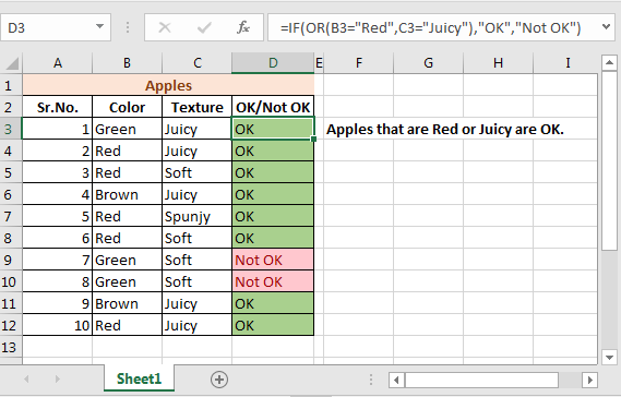
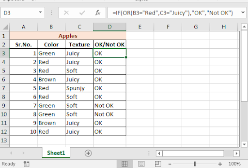
A fruit seller is selling apples. You will buy apples only if they are Red or Juicy. If an apple is not Red nor Juicy, you will not buy it.
Here we have two conditions and at least one of them need to be true to make you happy. Let’s write an IF OR formula for this in Excel 2016.
Implementation of IF with OR
Generic Formula
=IF(OR(condition1, condition2,…),value if true, value if false)
Example
Let’s consider the example we discussed in the beginning.
We have this table of apple’s colour and type.
If the colour is “Red” or type is “Juicy” then write OK in column D. If the color is not “Red”, nor the type is “Juicy” then type Not OK.

Write this IF OR formula in D2 column and drag it down.
=IF(OR(B3=»Red»,C3=»Juicy»),»OK»,»Not OK»)
And you can see now that only apples that are Red or Juicy are marked OK.
How It Works
IF Statement : You know how IF function in Excel works. It takes a boolean expression as first argument and returns one expression if TRUE and another if FALSE. Learn more about The Excel IF function.
=IF(TRUE or FALSE, statement if True, statement if false)
OR Function: Checks multiple conditions. Returns TRUE only if at least one of the conditions is TRUE else returns FALSE.
=OR(condition1, condition2,….) ==> TRUE/FALSE
In the end, OR function provides IF function TRUE or FALSE argument and based on that IF prints the result.
Alternate Solution:
Another way to do this is to use nested IFs for Multiple Conditions.
=IF(B3=»Red», “OK”, IF(C3=»Juicy»,”OK”,”Not OK”),”Not OK”)
Nested IF is good when we want different results but not when only one result. It will work but for multiple conditions, it will make your excel formula too long.
So here we learned about how to use IF with OR to check multiple conditions and show results if at least one of all conditions is TRUE. But what if you want to show results only if all condition is true. We will use AND function with IF in excel to do so.
Related Articles:
Excel OR function
Excel AND Function
IF with AND Function in Excel
Excel TRUE Function
Excel NOT function
IF not this or that in Microsoft Excel
IF with AND and OR function in Excel
Popular Articles:
The VLOOKUP Function in Excel
COUNTIF in Excel 2016
How to Use SUMIF Function in Excel
Logical functions are designed to test one or several conditions, and perform the actions prescribed for each of the two possible results. Such results can only be logical TRUE or FALSE.
Excel contains several logical functions such as IF, IFERROR, SUMIF, AND, OR, and others. The last two are not used in practice, as a rule, because the result of their calculations may be one of only two possible options (TRUE, FALSE). When combined with the IF function, they are able to significantly expand its functionality.
Examples of using formulas with IF, AND, OR functions in Excel
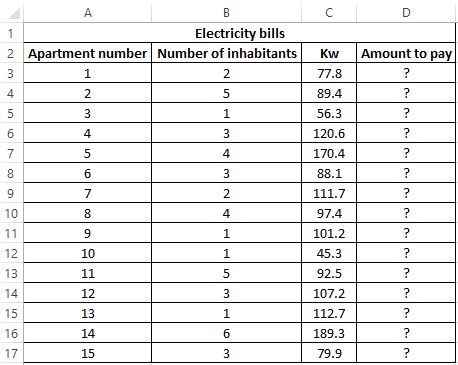
Example 1. When calculating the cost of the amount of consumed kW of electricity for subscribers, the following conditions are taken into account:
- If less than 3 people live in the apartment or less than 100 kW of electricity was consumed per month, the rate per 1 kW is 4.35$.
- In other cases, the rate for 1 kW is 5.25$.
Calculate the amount payable per month for several subscribers.
View source data table:
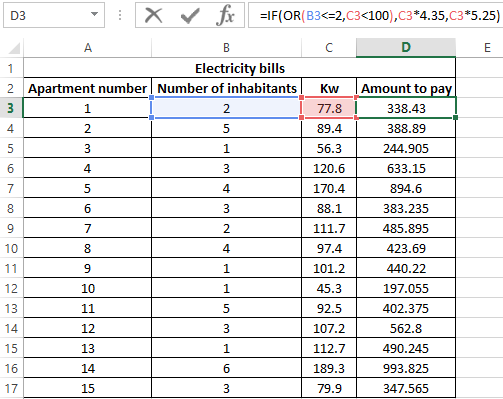
Perform the calculation according to the formula:
Argument Description:
- OR (B3<=2,C3<100) is a logical expression that verifies two conditions: do less than 3 people live in the apartment or does the total amount of energy consumed less than 100 kW? The result of the test will be TRUE if either of these two conditions is true;
- C3 * 4.35 — the amount to be paid, if the OR function returns TRUE;
- C3 * 5.25 is the amount to be paid if OR returns FALSE.
We stretch the formula for the remaining cells using the autocomplete function. The result of the calculation for each subscriber:
Using the AND function in the formula in the first argument in the IF function, we check the conformity of the values by two conditions at once.
Formula with IF and AVERAGE functions for selecting of values by conditions
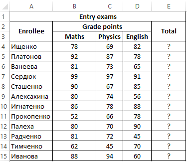
Example 2. Applicants entering the university for the specialty «mechanical engineer» are required to pass 3 exams in mathematics, physics and English. The maximum score for each exam is 100. The average passing score for 3 exams is 75, while the minimum score in physics must be at least 70 points, and in mathematics it is 80. Determine applicants who have successfully passed the exams.
View source table:
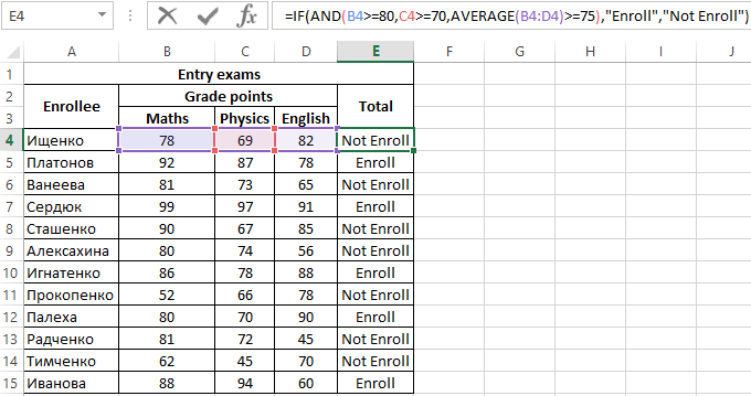
To determine the enrolled students use the formula:
Argument Description:
- AND(B4>=80,C4>=70,AVERAGE(B4:D4)>=75) — checked logical expressions according to the condition of the problem;
- «Enroll» — the result, if the function AND returned the value TRUE (all expressions represented as its arguments, as a result of the calculations returned the value TRUE);
- «Not Enroll» — the result if AND returned FALSE.
Using the autocomplete function (double-click on the cursor marker in the lower right corner), we get the rest of the results:
Formula with logical functions AND IF OR in excel
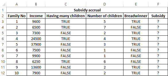
Example 3. Subsidies in the amount of 30% are charged to families with an average income below 8,000$, which are large or there is no main breadwinner. If the number of children is over 5, the amount of the subsidy is 50%. Determine who should receive subsidies and who should not.
View source table:
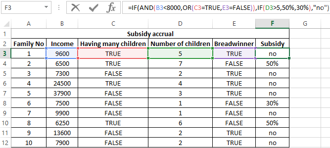
To check the criteria according to the condition of the problem, we write the formula:
Argument Description:
- AND(B3<8000,OR(C3=TRUE,E3=FALSE)) is the checked expression according to the condition of the problem. In this case, the AND function returns the TRUE value, if B3 <8000 is true and at least one of the expressions passed as arguments to the OR function also returns the TRUE value.
- The nested IF function performs a check on the number of children in the family, which rely on subsidies.
- If the main condition returned the result is FALSE, the main function IF returns the text string “no”.
Perform the calculation for the first family and stretch the formula to the remaining cells using the autocomplete function. Results:
Features of using logical functions IF, AND, OR in Excel
The IF function has the following syntax notation:
=IF(Logical_test,[ Value_if_True ],[ Value_if_False])
As you can see, by default, you can check only one condition, for example, is e3 more than 20? Using the IF function, this check can be done as follows:
=IF(EXP(3)>20,»more»,»less»)
As a result, the text string “more” will be returned. If we need to find out if any value belongs to the specified interval, we will need to compare this value with the upper and lower limits of the intervals, respectively. For example, is the result of calculating e3 in the range from 20 to 25? When using the IF function alone, you must enter the following entry:
=IF(EXP(3)>20,IF(EXP(3)<25,»belongs»,»does not belong»),»does not belong»)
We have a nested function IF as one of the possible results of the implementation of the main function IF, and therefore the syntax looks somewhat cumbersome. If you also need to know, for example, whether the square root e3 is equal to a numeric value from a fractional number range from 4 to 5, the final formula will look cumbersome and unreadable.
It is much easier to use as a condition a complex expression that can be written using AND and OR functions. For example, the above function can be rewritten as follows:
=IF(AND(EXP(3)>20,EXP(3)<25),»belongs»,»does not belong»)
The result of the execution of the AND expression (EXP(3)>20,EXP(3)<25) can be a logical value TRUE only if the result of checking each of the specified conditions is a logical value TRUE. In other words, the function AND allows you to test one, two or more hypotheses on their truth, and returns the result FALSE if at least one of them is incorrect.
Sometimes you want to know if at least one assumption is true. In this case, it is convenient to use the OR function, which performs the check of one or several logical expressions and returns a logical TRUE, if the result of the calculations of at least one of them is a logical TRUE. For example, you want to know if e3 is an integer or a number that is less than 100? To test this condition, you can use the following formula:
=IF(OR(MOD(EXP(3),1)<>0,EXP(3)<100),»true»,»false»)
The “<>” means inequality, that is, more or less than some value. In this case, both expressions return the value TRUE, and the result of the execution of the IF function is the text string «true.» However, if an OR test was performed (MOD(EXP (3),1)<>0,EXP(3)<20, while EXP(3) <20 will return FALSE, the result of the calculation of the IF function will not change, since MOD(EXP(3),1) <> 0 returns TRUE.
Download examples using the functions OR AND IF in Excel
In practice, often used bundles IF + AND, IF + OR, or all three functions at once. Consider examples of similar use of these functions.
To write an IF, AND, OR array formula in Excel 365, we must use the arithmetic operators * (multiplication) and + (addition). Why it’s so?
If we take the logical AND, OR with the IF in Excel 365 to spill the result, we won’t get our expected result.
I mean, such a formula won’t support a range/array in evaluation. Even if it supports, it won’t return an array result.
So we will replace the AND logical operator with the * (multiplication) and OR with the + (addition) arithmetic operators.
Coding the formula with the said two operators is very simple and easily readable.
I think I can convince you the same with the examples below.
Example to IF, AND, OR in Excel 365 (Non-Array Formula)
Imagine a user played a game three times, and we have recorded his scores out of 100 in cells A2, B2, and C2.
We want to perform the following three logical tests on the scores individually.
- If all scores are >=80, return OK.
- If any of the two scores are >=80, return OK.
- Finally, if any of the scores is >=80, return OK.
Logical Tests Using IF, AND, OR Functions
In Excel, we can perform the above three logical tests as follows.
1. E2 (If all scores are >=80, return OK)
=IF(AND(A2>=80,B2>=80,C2>=80),"OK","NOT OK")I have used the AND function with IF in the above Excel formula to test if all the three logical tests return TRUE.
2. F2 (If any of the two scores are >=80, return OK)
We must use the following logic (two parts) to test if any two logical tests return TRUE.
AND Part:-
a) Value 1>=80 and value 2>=80.
b) Value 1>=80 and value 3>=80.
c) Value 2>=80 and value 3>=80.
OR Part:-
a) The OR evaluates to TRUE if any two of the above three AND tests return TRUE.
So the formula will be as follows.
=IF(OR(AND(A2>=80,B2>=80),AND(A2>=80,C2>=80),AND(B2>=80,C2>=80)),"OK","NOT OK")It is an example of the IF, AND, OR logical test in Excel.
3. G2 (if any of the scores is >=80, return OK)
=IF(OR(A2>=80,B2>=80,C2>=80),"OK","NOT OK")Here I have used the OR function with IF to test if any of the three logical tests return TRUE.
As I have already mentioned, we can’t write an IF, AND, OR array formula as above in Excel 365.
Logical Tests Using IF, *, + Formula
Let’s substitute the above three formulas by replacing AND, OR with multiplication and addition.
But that’s not enough. Then?
The below formulas are self-explanatory.
1. E2 Formula
=IF((A2:A8>=80)*(B2:B8>=80)*(C2:C8>=80),"OK","NOT OK")How the multiplication replaces the logical function OR above?
Each test in the formula returns either TRUE or FALSE. If all the criteria are met, it will be =IF((TRUE*TRUE*TRUE),"OK","NOT OK").
We can even replace the multiplication operator here with addition.
=IF((A2:A8>=80)+(B2:B8>=80)+(C2:C8>=80)>2,"OK","NOT OK")Please remember that the value of TRUE is 1, and FALSE is 0.
2. F2 Formula
=IF((A2:A8>=80)+(B2:B8>=80)+(C2:C8>=80)>1,"OK","NOT OK")3. G2 Formula
=IF((A2:A8>=80)+(B2:B8>=80)+(C2:C8>=80)>0,"OK","NOT OK")Above I have tried to simplify the use of the logical operators within the IF function.
Now let’s open an Excel Spreadsheet and enter the scores of multiple players in the range A2:C8 as below.

So the values to evaluate are in cell range A2:C8.
I have inserted the following three IF, AND, OR array formulas in cells E2, F2, and G2, respectively.
1. E2 Array Formula
=IF((A2:A8>=80)*(B2:B8>=80)*(C2:C8>=80),"OK","NOT OK")2. F2 Array Formula
=IF((A2:A8>=80)+(B2:B8>=80)+(C2:C8>=80)>1,"OK","NOT OK")3. G2 Array Formula
=IF((A2:A8>=80)+(B2:B8>=80)+(C2:C8>=80)>0,"OK","NOT OK")If any of the above formulas return #SPILL!, please empty the cells down in that column.
Nested IF, AND, OR Combination in Excel 365
I want to assign grades based on the scores above.
In that case, we may require to write a nested IF, AND, OR combination array formula in Excel 365.
Here is how.
In the above example, we have used three formulas for the below three logical tests.
- If all scores are >=80, return OK.
- If any of the two scores are >=80, return OK.
- Finally, if any of the scores is >=80, return OK.
There each test returns OK or NOT OK.
Instead of that, here, I want the tests to return GR-1, GR-2, and GR-3.
- If all scores are >=80, return GR-1.
- If any of the two scores are >=80, return GR-2.
- Finally, if any of the scores is >=80, return GR-3.
For that, we should combine the above three IF, AND, OR Array Formulas.
How?
In the E2 formula, replace “OK” with “GR-1” and “NOT OK” with the F2 formula.
In that combined (E2 and F2) formula, replace “OK” with “GR-2” and “NOT OK” with the G2 formula.
Then, in the combined E2, F2, and G2 formula, replace “OK” with “GR-3” and replace “NOT OK” with “F.”
Here it is.

=IF(
     (A2:A8>=80)*(B2:B8>=80)*(C2:C8>=80),"GR-1",
     IF(
        (A2:A8>=80)+(B2:B8>=80)+(C2:C8>=80)>1,"GR-2",
        IF(
           (A2:A8>=80)+(B2:B8>=80)+(C2:C8>=80)>0,"GR-3","F"
        )
     )
)
We can call it a nested IF, AND, OR combination array formula.
Related:- How to Use the IFS Function in Excel 365.
Home / Excel Formulas / How to Combine IF and OR Functions in Excel
IF Function is one of the most powerful functions in excel. And, the best part is, that you can combine other functions with IF to increase its power.
Combining IF and OR functions is one of the most useful formula combinations in excel. In this post, I’ll show you why we need to combine IF and OR functions. And, why it’s highly useful for you.
Quick Intro
I am sure you have used both of these functions but let me give you a quick intro.
- IF – Use this function to test a condition. It will return a specific value if that condition is true, or else some other specific value if that condition is false.
- OR – Test multiple conditions. It will return true if any of those conditions is true, and false if all of those conditions are false.
The crux of both of the functions is IF function can test only one condition at a time. And, OR function can test multiple conditions but only return true/false. And, if we combine these two functions we can test multiple conditions with OR & return a specific value with IF.
How do IF and OR functions Work?
In the syntax of the IF function, have a logical test argument that we use to specify a condition to test.
IF(logical_test,value_if_true,value_if_false)
And, then it returns a value based on the result of that condition. Now, if we use OR function for that argument and specify multiple conditions for it.
If any of the conditions is true OR will return true and IF will return the specific value. And, if none of the conditions is true OR with return FALSE IF will return another specific value. In this way, we can test more than one value with the IF function. Let’s get into some real-life examples.
Examples
Here I have a table with stock details of two warehouses. Now the thing is I want to update the status in the table.
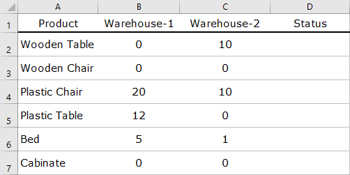
If there is no stock in both of the warehouses status should be “Out of Stock”. And, if there is stock in any of the warehouse status should be “In-Stocks”. So here I have to check two different conditions “Warehouse-1” & “Warehouse-2”.
And the formula will be.
=IF(OR(B2>0,C2>0),"In-Stock","Out of Stock")
In the above formula, if there is a value greater than zero in any of the cells (B2 & C2) OR function will return true, and IF will return the value “In-Stock”. But, if both cells have zero then OR will return false, and IF will return the value “Out of Stock”.
Download Sample File
- Ready
Last Words
Both of the functions are equally useful but when you combine them, you can use them in a better way. As I told you, by combining IF and Or functions you can test more than one condition. You can solve your two problems with this combination of functions.
And, if you want to Get Smarter than Your Colleagues check out these FREE COURSES to Learn Excel, Excel Skills, and Excel Tips and Tricks.