
The IF function allows you to make a logical comparison between a value and what you expect by testing for a condition and returning a result if that condition is True or False.
-
=IF(Something is True, then do something, otherwise do something else)
But what if you need to test multiple conditions, where let’s say all conditions need to be True or False (AND), or only one condition needs to be True or False (OR), or if you want to check if a condition does NOT meet your criteria? All 3 functions can be used on their own, but it’s much more common to see them paired with IF functions.
Use the IF function along with AND, OR and NOT to perform multiple evaluations if conditions are True or False.
Syntax
-
IF(AND()) — IF(AND(logical1, [logical2], …), value_if_true, [value_if_false]))
-
IF(OR()) — IF(OR(logical1, [logical2], …), value_if_true, [value_if_false]))
-
IF(NOT()) — IF(NOT(logical1), value_if_true, [value_if_false]))
|
Argument name |
Description |
|
|
logical_test (required) |
The condition you want to test. |
|
|
value_if_true (required) |
The value that you want returned if the result of logical_test is TRUE. |
|
|
value_if_false (optional) |
The value that you want returned if the result of logical_test is FALSE. |
|
Here are overviews of how to structure AND, OR and NOT functions individually. When you combine each one of them with an IF statement, they read like this:
-
AND – =IF(AND(Something is True, Something else is True), Value if True, Value if False)
-
OR – =IF(OR(Something is True, Something else is True), Value if True, Value if False)
-
NOT – =IF(NOT(Something is True), Value if True, Value if False)
Examples
Following are examples of some common nested IF(AND()), IF(OR()) and IF(NOT()) statements. The AND and OR functions can support up to 255 individual conditions, but it’s not good practice to use more than a few because complex, nested formulas can get very difficult to build, test and maintain. The NOT function only takes one condition.

Here are the formulas spelled out according to their logic:
|
Formula |
Description |
|---|---|
|
=IF(AND(A2>0,B2<100),TRUE, FALSE) |
IF A2 (25) is greater than 0, AND B2 (75) is less than 100, then return TRUE, otherwise return FALSE. In this case both conditions are true, so TRUE is returned. |
|
=IF(AND(A3=»Red»,B3=»Green»),TRUE,FALSE) |
If A3 (“Blue”) = “Red”, AND B3 (“Green”) equals “Green” then return TRUE, otherwise return FALSE. In this case only the first condition is true, so FALSE is returned. |
|
=IF(OR(A4>0,B4<50),TRUE, FALSE) |
IF A4 (25) is greater than 0, OR B4 (75) is less than 50, then return TRUE, otherwise return FALSE. In this case, only the first condition is TRUE, but since OR only requires one argument to be true the formula returns TRUE. |
|
=IF(OR(A5=»Red»,B5=»Green»),TRUE,FALSE) |
IF A5 (“Blue”) equals “Red”, OR B5 (“Green”) equals “Green” then return TRUE, otherwise return FALSE. In this case, the second argument is True, so the formula returns TRUE. |
|
=IF(NOT(A6>50),TRUE,FALSE) |
IF A6 (25) is NOT greater than 50, then return TRUE, otherwise return FALSE. In this case 25 is not greater than 50, so the formula returns TRUE. |
|
=IF(NOT(A7=»Red»),TRUE,FALSE) |
IF A7 (“Blue”) is NOT equal to “Red”, then return TRUE, otherwise return FALSE. |
Note that all of the examples have a closing parenthesis after their respective conditions are entered. The remaining True/False arguments are then left as part of the outer IF statement. You can also substitute Text or Numeric values for the TRUE/FALSE values to be returned in the examples.
Here are some examples of using AND, OR and NOT to evaluate dates.

Here are the formulas spelled out according to their logic:
|
Formula |
Description |
|---|---|
|
=IF(A2>B2,TRUE,FALSE) |
IF A2 is greater than B2, return TRUE, otherwise return FALSE. 03/12/14 is greater than 01/01/14, so the formula returns TRUE. |
|
=IF(AND(A3>B2,A3<C2),TRUE,FALSE) |
IF A3 is greater than B2 AND A3 is less than C2, return TRUE, otherwise return FALSE. In this case both arguments are true, so the formula returns TRUE. |
|
=IF(OR(A4>B2,A4<B2+60),TRUE,FALSE) |
IF A4 is greater than B2 OR A4 is less than B2 + 60, return TRUE, otherwise return FALSE. In this case the first argument is true, but the second is false. Since OR only needs one of the arguments to be true, the formula returns TRUE. If you use the Evaluate Formula Wizard from the Formula tab you’ll see how Excel evaluates the formula. |
|
=IF(NOT(A5>B2),TRUE,FALSE) |
IF A5 is not greater than B2, then return TRUE, otherwise return FALSE. In this case, A5 is greater than B2, so the formula returns FALSE. |

Using AND, OR and NOT with Conditional Formatting
You can also use AND, OR and NOT to set Conditional Formatting criteria with the formula option. When you do this you can omit the IF function and use AND, OR and NOT on their own.
From the Home tab, click Conditional Formatting > New Rule. Next, select the “Use a formula to determine which cells to format” option, enter your formula and apply the format of your choice.

Using the earlier Dates example, here is what the formulas would be.

|
Formula |
Description |
|---|---|
|
=A2>B2 |
If A2 is greater than B2, format the cell, otherwise do nothing. |
|
=AND(A3>B2,A3<C2) |
If A3 is greater than B2 AND A3 is less than C2, format the cell, otherwise do nothing. |
|
=OR(A4>B2,A4<B2+60) |
If A4 is greater than B2 OR A4 is less than B2 plus 60 (days), then format the cell, otherwise do nothing. |
|
=NOT(A5>B2) |
If A5 is NOT greater than B2, format the cell, otherwise do nothing. In this case A5 is greater than B2, so the result will return FALSE. If you were to change the formula to =NOT(B2>A5) it would return TRUE and the cell would be formatted. |
Note: A common error is to enter your formula into Conditional Formatting without the equals sign (=). If you do this you’ll see that the Conditional Formatting dialog will add the equals sign and quotes to the formula — =»OR(A4>B2,A4<B2+60)», so you’ll need to remove the quotes before the formula will respond properly.
Need more help?

See also
You can always ask an expert in the Excel Tech Community or get support in the Answers community.
Learn how to use nested functions in a formula
IF function
AND function
OR function
NOT function
Overview of formulas in Excel
How to avoid broken formulas
Detect errors in formulas
Keyboard shortcuts in Excel
Logical functions (reference)
Excel functions (alphabetical)
Excel functions (by category)
The logical IF statement in Excel is used for the recording of certain conditions. It compares the number and / or text, function, etc. of the formula when the values correspond to the set parameters, and then there is one record, when do not respond — another.
Logic functions — it is a very simple and effective tool that is often used in practice. Let us consider it in details by examples.
The syntax of the function «IF» with one condition
The operation syntax in Excel is the structure of the functions necessary for its operation data.
=IF(boolean;value_if_TRUE;value_if_FALSE)
Let us consider the function syntax:
- Boolean – what the operator checks (text or numeric data cell).
- Value_if_TRUE – what will appear in the cell when the text or numbers correspond to a predetermined condition (true).
- Value_if_FALSE – what appears in the box when the text or the number does not meet the predetermined condition (false).
Example:

Logical IF functions.
The operator checks the A1 cell and compares it to 20. This is a «Boolean». When the contents of the column is more than 20, there is a true legend «greater 20». In the other case it’s «less or equal 20».
Attention! The words in the formula need to be quoted. For Excel to understand that you want to display text values.
Here is one more example. To gain admission to the exam, a group of students must successfully pass a test. The results are listed in a table with columns: a list of students, a credit, an exam.

The statement IF should check not the digital data type but the text. Therefore, we prescribed in the formula В2= «done» We take the quotes for the program to recognize the text correctly.
The function IF in Excel with multiple conditions
Usually one condition for the logic function is not enough. If you need to consider several options for decision-making, spread operators’ IF into each other. Thus, we get several functions IF in Excel.
The syntax is as follows:
Here the operator checks the two parameters. If the first condition is true, the formula returns the first argument is the truth. False — the operator checks the second condition.
Examples of a few conditions of the function IF in Excel:

It’s a table for the analysis of the progress. The student received 5 points:
- А – excellent;
- В – above average or superior work;
- C – satisfactory;
- D – a passing grade;
- E – completely unsatisfactory.
IF statement checks two conditions: the equality of value in the cells.

In this example, we have added a third condition, which implies the presence of another report card and «twos». The principle of the operator is the same.
Enhanced functionality with the help of the operators «AND» and «OR»
When you need to check out a few of the true conditions you use the function И. The point is: IF A = 1 AND A = 2 THEN meaning в ELSE meaning с.
OR function checks the condition 1 or condition 2. As soon as at least one condition is true, the result is true. The point is: IF A = 1 OR A = 2 THEN value B ELSE value C.
Functions AND & OR can check up to 30 conditions.
An example of using the operator AND:

It’s the example of using the logical operator OR.

How to compare data in two tables
Users often need to compare the two spreadsheets in an Excel to match. Examples of the «life»: compare the prices of goods in different bringing, to compare balances (accounting reports) in a few months, the progress of pupils (students) of different classes, in different quarters, etc.
To compare the two tables in Excel, you can use the COUNTIFS statement. Consider the order of application functions.
For example, consider the two tables with the specifications of various food processors. We planned allocation of color differences. This problem in Excel solves the conditional formatting.
Baseline data (tables, which will work with):

Select the first table. Conditional Formatting — create a rule — use a formula to determine the formatted cells:

In the formula bar write: = COUNTIFS (comparable range; first cell of first table)=0. Comparing range is in the second table.
To drive the formula into the range, just select it first cell and the last. «= 0» means the search for the exact command (not approximate) values.
Choose the format and establish what changes in the cell formula in compliance. It’s better to do a color fill.
Select the second table. Conditional Formatting — create a rule — use the formula. Use the same operator (COUNTIFS). For the second table formula:
Download all examples in Excel

Now it is easy to compare the characteristics of the data in the table.
What to Know
- The syntax of IF-THEN is =IF(logic test,value if true,value if false).
- The first argument tells the function what to do if the comparison is true.
- The second argument tells the function what to do if the comparison is false.
This article explains how to use the IF-THEN function in Excel for Microsoft 365, Excel 2019, 2016, 2013, 2010; Excel for Mac, and Excel Online, as well as a few examples.
Inputting IF-THEN in Excel
The IF-THEN function in Excel is a powerful way to add decision making to your spreadsheets. It tests a condition to see if it’s true or false and then carries out a specific set of instructions based on the results.
For example, by inputting an IF-THEN in Excel, you can test if a specific cell is greater than 900. If it is, you can make the formula return the text «PERFECT.» If it isn’t, you can make the formula return «TOO SMALL.»
There are many conditions you can enter into the IF-THEN formula.
The IF-THEN function’s syntax includes the name of the function and the function arguments inside of the parenthesis.
This is the proper syntax of the IF-THEN function:
=IF(logic test,value if true,value if false)
The IF part of the function is the logic test. This is where you use comparison operators to compare two values.
The THEN part of the function comes after the first comma and includes two arguments separated by a comma.
- The first argument tells the function what to do if the comparison is true.
- The second argument tells the function what to do if the comparison is false.
A Simple IF-THEN Function Example
Before moving on to more complex calculations, let’s look at a straightforward example of an IF-THEN statement.
Our spreadsheet is set up with cell B2 as $100. We can input the following formula into C2 to indicate whether the value is larger than $1000.
=IF(B2>1000,"PERFECT","TOO SMALL")
This function has the following arguments:
- B2>1000 tests whether the value in cell B2 is larger than 1000.
- «PERFECT» returns the word PERFECT in cell C2 if B2 is larger than 1000.
- «TOO SMALL» returns the phrase TOO SMALL in cell C2 if B2 is not larger than 1000.
The comparison part of the function can compare only two values. Either of those two values can be:
- Fixed number
- A string of characters (text value)
- Date or time
- Functions that return any of the values above
- A reference to any other cell in the spreadsheet containing any of the above values
The TRUE or FALSE part of the function can also return any of the above. This means that you can make the IF-THEN function very advanced by embedding additional calculations or functions inside of it (see below).
When inputting true or false conditions of an IF-THEN statement in Excel, you need to use quotation marks around any text you want to return, unless you’re using TRUE and FALSE, which Excel automatically recognizes. Other values and formulas don’t require quotation marks.
Inputting Calculations Into the IF-THEN Function
You can embed different calculations for the IF-THEN function to perform, depending on the comparison results.
In this example, one calculation is used to calculate the tax owed, depending on the total income in B2.
The logic test compares total income in B2 to see if it’s greater than $50,000.00.
=IF(B2>50000,B2*0.15,B2*0.10)
In this example, B2 is not larger than 50,000, so the «value_if_false» condition will calculate and return that result.
In this case, that’s B2*0.10, which is 4000.
The result is placed into cell C2, where the IF-THEN function is inserted, will be 4000.
You can also embed calculations into the comparison side of the function.
For example, if you want to estimate that taxable income will only be 80% of total income, you could change the above IF-THEN function to the following.
=IF(B2*0.8>50000,B2*0.15,B2*0.10)
This will perform the calculation on B2 before comparing it to 50,000.
Never enter a comma when entering numbers in the thousands. This is because Excel interprets a comma as the end of an argument inside of a function.
Nesting Functions Inside of an IF-THEN Function
You can also embed (or «nest») a function inside of an IF-THEN function.
This lets you perform advanced calculations and then compare the actual results to the expected results.
In this example, let’s say you have a spreadsheet with five students’ grades in column B. You could average those grades using the AVERAGE function. Depending on the class average results, you could have cell C2 return either «Excellent!» or «Needs Work.»
This is how you would input that IF-THEN function:
=IF(AVERAGE(B2:B6)>85,"Excellent!","Needs Work")
This function returns the text «Excellent!» in cell C2 if the class average is over 85. Otherwise, it returns «Needs Work.»
As you can see, inputting the IF-THEN function in Excel with embedded calculations or functions allows you to create dynamic and highly functional spreadsheets.
FAQ
-
How do I create multiple IF-THEN statements in Excel?
-
How many IF statements can you nest in Excel?
You can nest up to 7 IF statements within a single IF-THEN statement.
-
How does conditional formatting work in Excel?
With conditional formatting in Excel, you can apply more than one rule to the same data to test for different conditions. Excel first determines if the various rules conflict, and, if so, the program determines which conditional formatting rule to apply to the data.
Thanks for letting us know!
Get the Latest Tech News Delivered Every Day
Subscribe
To perform complicated and powerful data analysis, you need to test various conditions at a single point in time. The data analysis might require logical tests also within these multiple conditions.
For this, you need to perform Excel if statement with multiple conditions or ranges that include various If functions in a single formula.
Those who use Excel daily are well versed with Excel If statement as it is one of the most-used formula. Here you can check various Excel If or statement, Nested If, AND function, Excel IF statements, and how to use them. We have also provided a VIDEO TUTORIAL for different If Statements.
There are various If statements available in Excel. You have to know which of the Excel If you will work at what condition. Here you can check multiple conditions where you can use Excel If statement.
1) Excel If Statement
If you want to test a condition to get two outcomes then you can use this Excel If statement.
=If(Marks>=40, “Pass”)
2) Nested If Statement
Let’s take an example that met the below-mentioned condition
- If the score is between 0 to 60, then Grade F
- If the score is between 61 to 70, then Grade D
- If the score is between 71 to 80, then Grade C
- If the score is between 81 to 90, then Grade B
- If the score is between 91 to 100, then Grade A
Then to test the condition the syntax of the formula becomes,
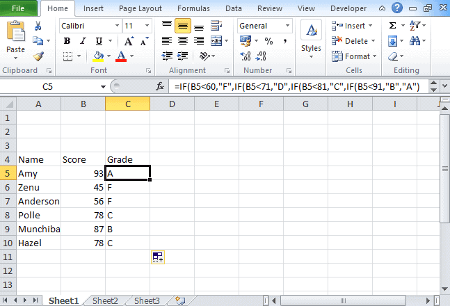
=If(B5<60, “F”,If(B5<71, “D”, If(B5<81,”C”,If(B5<91,”B”,”A”)
3) Excel If with Logical Test
There are 2 different types of conditions AND and OR. You can use the IF statement in excel between two values in both these conditions to perform the logical test.
AND Function: If you are performing the logical test based on AND function, then excel will give you TRUE as an outcome in every condition else it will return false.
OR Function: If you are using OR condition for the logical test, then excel will give you an outcome as TRUE if any of the situations match else it returns false.
For this, multiple testing is to be done using AND and OR function, you should gain expertise in using either or both of these with IF statement. Here we have used if the function with 3 conditions.
How to apply IF & AND function in Excel
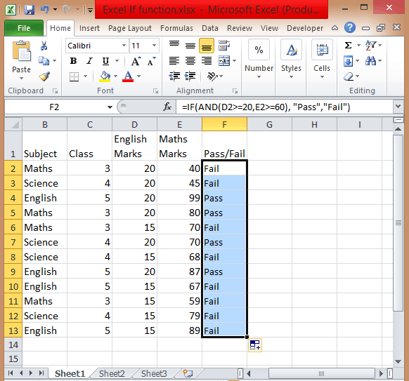
- To perform this multiple if and statements in excel, we will take the data set for the student’s marks that contain fields such as English and Math’s Marks.
- The score of the English subject is stored in the D column whereas the Maths score is stored in column E.
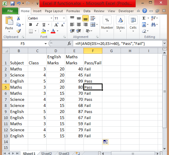
- Let say a student passes the class if his or her score in English is greater than or equal to 20 and he or she scores more than 60 in Maths.
- To create a report in matters of seconds, if formula combined with AND can suffice.
- Type =IF( Excel will display the logical hint just below the cell F2. The parameters of this function are logical_test, value_if_true, value_if_false.
- The first parameter contains the condition to be matched. You can use multiple If and AND conditions combined in this logical test.
- In the second parameter, type the value that you want Excel to display if the condition is true. Similarly, in the third parameter type the value that will be displayed if your condition is false.

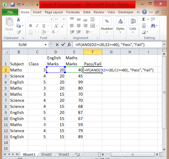
- Apply If & And formula, you will get =IF(AND(D2>=20,E2>=60),”Pass”,”Fail”).
![]()
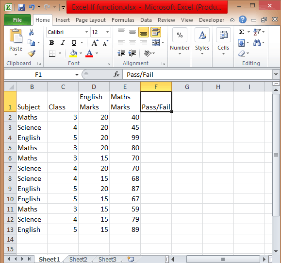
- Add Pass/Fail column in the current table.

- After you have applied this formula, you will find the result in the column.
- Copy the formula from cell F2 and paste in all other cells from F3 to F13.

How to use If with Or function in Excel
To use If and Or statement excel, you need to apply a similar formula as you have applied for If & And with the only difference is that if any of the condition is true then it will show you True.
To apply the formula, you have to follow the above process. The formula is =IF((OR(D2>=20, E2>=60)), “Pass”, “Fail”). If the score is equal or greater than 20 for column D or the second score is equal or greater than 60 then the person is the pass.
How to Use If with And & Or function
If you want to test data based on several multiple conditions then you have to apply both And & Or functions at a single point in time. For example,
Situation 1: If column D>=20 and column E>=60
Situation 2: If column D>=15 and column E>=60
If any of the situations met, then the candidate is passed, else failed. The formula is
=IF(OR(AND(D2>=20, E2>=60), AND(D2>=20, E2>=60)), “Pass”, “Fail”).
4) Excel If Statement with other functions
Above we have learned how to use excel if statement multiple conditions range with And/Or functions. Now we will be going to learn Excel If Statement with other excel functions.
- Excel If with Sum, Average, Min, and Max functions
Let’s take an example where we want to calculate the performance of any student with Poor, Satisfactory, and Good.
If the data set has a predefined structure that will not allow any of the modifications. Then you can add values with this If formula:
=If((A2+B2)>=50, “Good”, If((A2+B2)=>30, “Satisfactory”, “Poor”))
Using the Sum function,
=If(Sum(A2:B2)>=120, “Good”, If(Sum(A2:B2)>=100, “Satisfactory”, “Poor”))
Using the Average function,
=If(Average(A2:B2)>=40, “Good”, If(Average(A2:B2)>=25, “Satisfactory”, “Poor”))
Using Max/Min,
If you want to find out the highest scores, using the Max function. You can also find the lowest scores using the Min function.
=If(C2=Max($C$2:$C$10), “Best result”, “ “)
You can also find the lowest scores using the Min function.
=If(C2=Min($C$2:$C$10), “Worst result”, “ “)
If we combine both these formulas together, then we get
=If(C2=Max($C$2:$C$10), “Best result”, If(C2=Min($C$2:$C$10), “Worst result”, “ “))
You can also call it as nested if functions with other excel functions. To get a result, you can use these if functions with various different functions that are used in excel.
So there are four different ways and types of excel if statements, that you can use according to the situation or condition. Start using it today.
So this is all about Excel If statement multiple conditions ranges, you can also check how to add bullets in excel in our next post.
I hope you found this tutorial useful
You may also like the following Excel tutorials:
- Multiple If Statements in Excel
- Excel Logical test
- How to Compare Two Columns in Excel (using VLOOKUP & IF)
- Using IF Function with Dates in Excel (Easy Examples)
What is IF Function in Excel?
IF function in Excel evaluates whether a given condition is met and returns a value depending on whether the result is “true” or “false”. It is a conditional function of Excel, which returns the result based on the fulfillment or non-fulfillment of the given criteria.
For example, the IF formula in Excel can be applied as follows:
“=IF(condition A,“value B”,“value C”)”
The IF excel function returns “value B” if condition A is met and returns “value C” if condition A is not met.
It is often used to make logical interpretations which help in decision-making.
Table of contents
- What is IF Function in Excel?
- Syntax of the IF Excel Function
- How to Use IF Function in Excel?
- Example #1
- Example #2
- Example #3
- Example #4
- Example #5
- Guidelines for the Multiple IF Statements
- Frequently Asked Question
- IF Excel Function Video
- Recommended Articles
Syntax of the IF Excel Function
The syntax of the IF function is shown in the following image:

The IF excel function accepts the following arguments:
- Logical_test: It refers to the condition to be evaluated. The condition can be a value or a logical expression.
- Value_if_true: It is the value returned as a result when the condition is “true”.
- Value_if_false: It is the value returned as a result when the condition is “false”.
In the formula, the “logical_test” is a required argument, whereas the “value_if_true” and “value_if_false” are optional arguments.
The IF formula uses logical operators to evaluate the values in a range of cells. The following table shows the different logical operatorsLogical operators in excel are also known as the comparison operators and they are used to compare two or more values, the return output given by these operators are either true or false, we get true value when the conditions match the criteria and false as a result when the conditions do not match the criteria.read more and their meaning.
| Operator | Meaning |
|---|---|
| = | Equal to |
| > | Greater than |
| >= | Greater than or equal to |
| < | Less than |
| <= | Less than or equal to |
| <> | Not equal to |
How to Use IF Function in Excel?
Let us understand the working of the IF function with the help of the following examples in Excel.
You can download this IF Function Excel Template here – IF Function Excel Template
Example #1
If there is no oxygen on a planet, life is impossible. If oxygen is available on a planet, then life is possible. The following table shows a list of planets in column A and the information on the availability of oxygen in column B. We have to find the planets where life is possible, based on the condition of oxygen availability.

Let us apply the IF formula to cell C2 to find out whether life is possible on the planets listed in the table.
The IF formula is stated as follows:
“=IF(B2=“Yes”, “Life is Possible”, “Life is Not Possible”)
The succeeding image shows the IF formula applied to cell C2.

The subsequent image shows how the IF formula is applied to the range of cells C2:C5.

Drag the cells to view the output of all the planets.

The output in the below worksheet shows life is possible on the planet Earth.
Flow Chart of Generic IF Excel Function

The IF Function Flow Chart for Mars (Example #1)

The flow of IF function flowchart for Jupiter and Venus is the same as the IF function flowchart for Mars (Example #1).
The IF Function Flow Chart for Earth

Hence, the IF excel function allows making logical comparisons between values. The modus operandi of the IF function is stated as: If something is true, then do something; otherwise, do something else.
Example #2
The following table shows a list of years. We want to find out if the given year is a leap year or not.
A leap year has 366 days; the extra day is the 29th of February. The criteria for a leap year are stated as follows:
- The year will be exactly divisible by 4 and not exactly be divisible by 100 or
- The year will be exactly divisible by 400.

In this example, we will use the IF function along with the AND, OR, and MOD functions to find the leap years.
We use the MOD function to find a remainder after a dividend is divided by a divisor.
The AND functionThe AND function in Excel is classified as a logical function; it returns TRUE if the specified conditions are met, otherwise it returns FALSE.read more evaluates both the conditions of the leap years for the value “true”. The OR functionThe OR function in Excel is used to test various conditions, allowing you to compare two values or statements in Excel. If at least one of the arguments or conditions evaluates to TRUE, it will return TRUE. Similarly, if all of the arguments or conditions are FALSE, it will return FASLE.read more evaluates either of the condition for the value “true”.
We will apply the MOD function to the conditions as follows:
If MOD(year,4)=0 and MOD(year,100)<>(is not equal to) 0, then the year is a leap year.
or
If MOD(year,400)=0, then the year is a leap year; otherwise, the year is not a leap year.
The IF formula is stated as follows:
“=IF(OR(AND((MOD(year,4)=0),(MOD(year,100)<>0)),(MOD(year,400)=0)),“Leap Year”, “Not A Leap Year”)”
The argument “year” refers to a reference value.
The following images show the output of the IF formula applied in the range of cells.


The following image shows how the IF formula is applied to the range of cells B2:B18.

The succeeding table shows the years 1960, 2028, and 2148 as leap years and the remaining as non-leap years.

The result of the IF excel formula is displayed for the range of cells B2:B18 in the following image.

Example #3
The succeeding table shows a list of drivers and the directions they undertook to reach the destination. It is preceded by an image of the road intersection explaining the turns taken by the drivers and their destinations. The right turn leads to town B, and the left turn leads to town C. Identify the driver’s destination to town B and town C.
Road Intersection Image


Let us apply the IF excel function to find the destination. Here, the condition is mentioned as follows:
- If the driver turns right, he/she reaches town B.
- If the driver turns left, he/she reaches town C.
We use the following IF formula to find the destination:
“=IF(B2=“Left”, “Town C”, “Town B”)”
The succeeding image shows the output of the IF formula applied to cell C2.

Drag the cells to use the formula in the range C2:C11. Finally, we get the destinations of each driver for their turning movements.
The below image displays the IF formula applied to the range.

The output of the IF formula and the destinations are displayed in the succeeding image.

The result shows that six drivers reached town C, and the remaining four have reached town B.
Example #4
The following table shows a list of items and their inventory levels. We want to check if the specific item is available in the inventory or not using the IF function.

Let us list the name of items in column A and the number of items in column B. The list of data to be validated for the entire items list is shown in the cell E2 of the below image.

We use the Excel IF along with the VLOOKUP functionThe VLOOKUP excel function searches for a particular value and returns a corresponding match based on a unique identifier. A unique identifier is uniquely associated with all the records of the database. For instance, employee ID, student roll number, customer contact number, seller email address, etc., are unique identifiers.
read more to check the availability of the items in the inventory.
The VLOOKUP function looks up the values referring to the number of items, and the IF function will check whether the item number is greater than zero or not.
We will apply the following IF formula in the F2 cell:
“=IF(VLOOKUP(E2,A2:B11,2,0)=0, “Item Not Available”,“Item Available”)”
If the lookup value of an item is equal to 0, then the item is not available; else, the item is available.
The succeeding image shows the result of the IF formula in the cell F2.

Select “bat” in the E2 item cell to know whether the item is available or not in the inventory (as shown in the following image).

Example #5
The following table shows the list of students and their marks. The grade criteria are provided based on the marks obtained by the students. We want to find the grade of each student in the list.

We apply the Nested IF in Excel since we have multiple criteria to find and decide each student’s grade.
The Nesting of IF function uses the IF function inside another IF formula when multiple conditions are to be fulfilled.
The syntax of Nesting of IF function is stated as follows:
“=IF( condition1, value_if_true1, IF( condition2, value_if_true2, value_if_false2 ))”
The succeeding table represents the range of scores and the grades, respectively.

Let us apply the multiple IF conditions with AND function in the below-nested formula to find out the grade of the students:
“=IF((B2>=95),“A”,IF(AND(B2>=85,B2<=94),“B”,IF(AND(B2>=75,B2<=84),“C”,IF(AND(B2>=61,B2<=74),“D”,“F”))))”
The IF function checks the logical condition as shown in the formula below:
“=IF(logical_test, [value_if_true],[value_if_false])”
We will split the above-mentioned nested formula and check the IF statements as shown below:
First Logical Test: B2>=95
If the formula returns,
- Value_if_true, execute: “A” (Grade A) else(comma) enter value_if_false
- Value_if_false, then the formula finds another IF condition and enter IF condition
Second Logical Test: B2>=85(logical expression 1) and B2<=94(logical expression 2)
(We use AND function to check the multiple logical expressions as the two given conditions are to be evaluated for “true.”)
If the formula returns,
- Value_if_true, execute: “B” (Grade B) else(comma) enter value_if_false
- Value_if_false, then the formula finds another IF condition and enter IF condition
Third Logical Test: B2>=75(logical expression 1) and B2<=84(logical expression 2)
(We use AND function to check the multiple logical expressions as the two given conditions are to be evaluated for “true.”)
If the formula returns,
- Value_if_true, execute: “C” (Grade C) else(comma) enter value_if_false
- value_if_false, then the formula finds another IF condition and enter IF condition
Fourth Logical Test: B2>=61(logical expression 1) and B2<=74(logical expression 2)
(We use AND function to check the multiple logical expressions as the two given conditions are to be evaluated for “true.”)
If the formula returns,
- Value_if_true, execute: “D” (Grade D) else(comma) enter value_if_false
- Value_if_false, execute: “F” (Grade F)
- Finally, close the parenthesis.
The below image displays the output of the IF formula applied to the range.

The succeeding image shows the IF nested formula applied to the range.

The grades of the students are listed in the following table.

Guidelines for the Multiple IF Statements
The guidelines for the multiple IF statements are listed as follows:
- Use nested IF function to a limited extent as multiple IF statements require a great deal of thought to be accurate.
- Multiple IF statementsIn Excel, multiple IF conditions are IF statements that are contained within another IF statement. They are used to test multiple conditions at the same time and return distinct values. Additional IF statements can be included in the ‘value if true’ and ‘value if false’ arguments of a standard IF formula.read more require multiple parentheses (), which is often difficult to manage. Excel provides a way to check the color of each opening and closing parenthesis to avoid this situation. The last closing parenthesis color will always be black, denoting the end of the formula statement.
- Whenever we pass a string value for the arguments “value_if_true” and “value_if_false” or test a reference against a string value, enclose the string value in double quotes. Passing a string value without quotes will result in “#NAME?” error.
Frequently Asked Question
1. What is the IF function in Excel?
The Excel IF function is a logical function that checks the given criteria and returns one value for a “true” and another value for a “false” result.
The syntax of the IF function is stated as follows:
“=IF(logical_test, [value_if_true], [value_if_false])”
The arguments are as follows:
1. Logical_test – It refers to a value or condition that is tested.
2. Value_if_true – It is the value returned when the condition logical_test is “true.”
3. Value_if_false – It is the value returned when the condition logical_test is “false.”
The “logical_test” is a required argument, whereas the “value_if_true” and “value_if_false” are optional arguments.
2. How to use the IF Excel function with multiple conditions?
The IF Excel statement for multiple conditions is created by using multiple IF functions in a single formula.
The syntax of IF function with multiple conditions is stated as follows:
“=IF (condition 1_“true”, do something, IF (condition 2_“true”, do something, IF (condition 3_ “true”, do something, else do something)))”
3. How to use the function IFERROR in Excel?
IF Excel Function Video
Recommended Articles
This has been a guide to the IF function in Excel. Here we discuss how to use the IF function along with examples and downloadable templates. You may also look at these useful functions –
- What is the Logical Test in Excel?A logical test in Excel results in an analytical output, either true or false. The equals to operator, “=,” is the most commonly used logical test.read more
- “Not Equal to” in Excel“Not Equal to” argument in excel is inserted with the expression <>. The two brackets posing away from each other command excel of the “Not Equal to” argument, and the user then makes excel checks if two values are not equal to each other.read more
- Data Validation ExcelThe data validation in excel helps control the kind of input entered by a user in the worksheet.read more