
Содержание
- Excel Nested IF statement: examples, best practices and alternatives
- Excel nested IF statement
- Nested IF with OR/AND conditions
- Nested IF in Excel with OR statements
- Nested IF in Excel with AND statements
- VLOOKUP instead of nested IF in Excel
- IFS statement as alternative to nested IF function
- CHOOSE instead of nested IF formula in Excel
- SWITCH function as a concise form of nested IF in Excel
- Concatenating multiple IF functions in Excel
- Excel conditional formatting formulas based on another cell
- Excel conditional formatting based on another cell value
- How to create a conditional formatting rule based on formula
- Excel conditional formatting formula examples
- Formulas to compare values (numbers and text)
- AND and OR formulas
- Conditional formatting for empty and non-empty cells
- Excel formulas to work with text values
- Excel formulas to highlight duplicates
- Highlight duplicates including 1 st occurrences
- Highlight duplicates without 1 st occurrences
- Highlight consecutive duplicates in Excel
- Highlight duplicate rows
- Compare 2 columns for duplicates
- Formulas to highlight values above or below average
- How to highlight the nearest value in Excel
- Example 1. Find the nearest value, including exact match
- Example 2. Highlight a value closest to the given value, but NOT exact match
- Why isn’t my Excel conditional formatting working correctly?
Excel Nested IF statement: examples, best practices and alternatives
 by Svetlana Cheusheva, updated on March 16, 2023
The tutorial explains how to use the nested IF function in Excel to check multiple conditions. You will also learn a few other functions that could be good alternatives to using a nested formula in Excel.
How do you usually implement a decision-making logic in your Excel worksheets? In most cases, you’d use an IF formula to test your condition and return one value if the condition is met, another value if the condition is not met. To evaluate more than one condition and return different values depending on the results, you nest multiple IFs inside each other.
Though very popular, the nested IF statement is not the only way to check multiple conditions in Excel. In this tutorial, you will find a handful of alternatives that are definitely worth exploring.
Excel nested IF statement
Here’s the classic Excel nested IF formula in a generic form:
You can see that each subsequent IF function is embedded into the value_if_false argument of the previous function. Each IF function is enclosed in its own set of parentheses, but all the closing parentheses are at the end of the formula.
Our generic nested IF formula evaluates 3 conditions, and returns 4 different results (result 4 is returned if none of the conditions is TRUE). Translated into a human language, this nested IF statement tells Excel to do the following:
As an example, let’s find out commissions for a number of sellers based on the amount of sales they’ve made:
| Commission | Sales |
| 3% | $1 — $50 |
| 5% | $51 — $100 |
| 7% | $101 — $150 |
| 10% | Over $150 |
In math, changing the order of addends does not change the sum. In Excel, changing the order of IF functions changes the result. Why? Because a nested IF formula returns a value corresponding to the first TRUE condition. Therefore, in your nested IF statements, it’s very important to arrange the conditions in the right direction — high to low or low to high, depending on your formula’s logic. In our case, we check the «highest» condition first, then the «second highest», and so on:
=IF(B2>150, 10%, IF(B2>=101, 7%, IF(B2>=51, 5%, IF(B2>=1, 3%, «»)))) 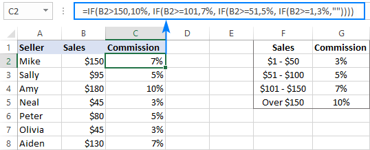
If we placed the conditions in the reverse order, from the bottom up, the results would be all wrong because our formula would stop after the first logical test (B2>=1) for any value greater than 1. Let’s say, we have $100 in sales — it is greater than 1, so the formula would not check other conditions and return 3% as the result.
If you’d rather arrange the conditions from low to high, then use the «less than» operator and evaluate the «lowest» condition first, then the «second lowest», and so on:
As you see, it takes quite a lot of thought to build the logic of a nested IF statement correctly all the way to the end. And although Microsoft Excel allows nesting up to 64 IF functions in one formula, it is not something you’d really want to do in your worksheets. So, if you (or someone else) are gazing at your Excel nested IF formula trying to figure out what it actually does, it’s time to reconsider your strategy and probably choose another tool in your arsenal.
Nested IF with OR/AND conditions
In case you need to evaluate a few sets of different conditions, you can express those conditions using OR as well as AND function, nest the functions inside IF statements, and then nest the IF statements into each other.
Nested IF in Excel with OR statements
By using the OR function you can check two or more different conditions in the logical test of each IF function and return TRUE if any (at least one) of the OR arguments evaluates to TRUE. To see how it actually works, please consider the following example.
Supposing, you have two columns of sales, say January sales in column B and February sales in column C. You wish to check the numbers in both columns and calculate the commission based on a higher number. In other words, you build a formula with the following logic: if either Jan or Feb sales are greater than $150, the seller gets 10% commission, if Jan or Feb sales are greater than or equal to $101, the seller gets 7% commission, and so on.
To have it done, write a few OF statements like OR(B2>150, C2>150) and nest them into the logical tests of the IF functions discussed above. As the result, you get this formula:
=IF(OR(B2>150, C2>150), 10%, IF(OR(B2>=101, C2>=101),7%, IF(OR(B2>=51, C2>=51), 5%, IF(OR(B2>=1, C2>=1), 3%, «»))))
And have the commission assigned based on the higher sales amount: 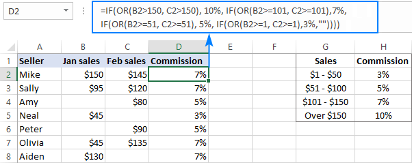
For more formula examples, please see Excel IF OR statement.
Nested IF in Excel with AND statements
If your logical tests include multiple conditions, and all of those conditions should evaluate to TRUE, express them by using the AND function.
For example, to assign the commissions based on a lower number of sales, take the above formula and replace OR with AND statements. To put it differently, you tell Excel to return 10% only if Jan and Feb sales are greater than $150, 7% if Jan and Feb sales are greater than or equal to $101, and so on.
=IF(AND(B2>150, C2>150), 10%, IF(AND(B2>=101, C2>=101), 7%, IF(AND(B2>=51, C2>=51), 5%, IF(AND(B2>=1, C2>=1), 3%, «»))))
As the result, our nested IF formula calculates the commission based on the lower number in columns B and C. If either column is empty, there is no commission at all because none of the AND conditions is met: 
If you’d like to return 0% instead of blank cells, replace an empty string (»») in the last argument with 0%:
=IF(AND(B2>150, C2>150), 10%, IF(AND(B2>=101, C2>=101), 7%, IF(AND(B2>=51, C2>=51), 5%, IF(AND(B2>=1, C2>=1), 3%, 0%)))) 
VLOOKUP instead of nested IF in Excel
When you are dealing with «scales», i.e. continuous ranges of numerical values that together cover the entire range, in most cases you can use the VLOOKUP function instead of nested IFs.
For starters, make a reference table like shown in the screenshot below. And then, build a Vlookup formula with approximate match, i.e. with the range_lookup argument set to TRUE.
Assuming the lookup value is in B2 and the reference table is F2:G5, the formula goes as follows:
Please notice that we fix the table_array with absolute references ($F$2:$G$5) for the formula to copy correctly to other cells: 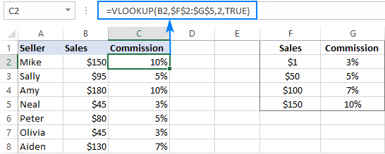
By setting the last argument of your Vlookup formula to TRUE, you tell Excel to search for the closest match — if an exact match is not found, return the next largest value that is smaller than the lookup value. As the result, your formula will match not only the exact values in the lookup table, but also any values that fall in between.
For example, the lookup value in B3 is $95. This number does not exist in the lookup table, and Vlookup with exact match would return an #N/A error in this case. But Vlookup with approximate match continues searching until it finds the nearest value that is less than the lookup value (which is $50 in our example) and returns a value from the second column in the same row (which is 5%).
But what if the lookup value is less than the smallest number in the lookup table or the lookup cell is empty? In this case, a Vlookup formula will return the #N/A error. If it’s not what you actually want, nest VLOOKUP inside IFERROR and supply the value to output when the lookup value is not found. For example:
=IFERROR(VLOOKUP(B2, $F$2:$G$5, 2, TRUE), «Outside range»)
Important note! For a Vlookup formula with approximate match to work correctly, the first column in the lookup table must be sorted in ascending order, from smallest to largest.
IFS statement as alternative to nested IF function
In Excel 2016 and later versions, Microsoft introduced a special function to evaluate multiple conditions — the IFS function.
An IFS formula can handle up to 127 logical_test/value_if_true pairs, and the first logical test that evaluates to TRUE «wins»:
In accordance with the above syntax, our nested IF formula can be reconstructed in this way:
=IFS(B2>150, 10%, B2>=101, 7%, B2>=51, 5%, B2>0, 3%)
Please pay attention that the IFS function returns the #N/A error if none of the specified conditions is met. To avoid this, you can add one more logical_test/value_if_true to the end of your formula that will return 0 or empty string («») or whatever value you want if none of the previous logical tests is TRUE:
=IFS(B2>150, 10%, B2>=101, 7%, B2>=51, 5%, B2>0, 3%, TRUE, «»)
As the result, our formula will return an empty string (blank cell) instead of the #N/A error if a corresponding cell in column B is empty or contains text or negative number. 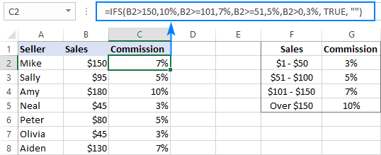
Note. Like nested IF, Excel’s IFS function returns a value corresponding to the first condition that evaluates to TRUE, which is why the order of logical tests in an IFS formula matters.
CHOOSE instead of nested IF formula in Excel
Another way to test multiple conditions within a single formula in Excel is using the CHOOSE function, which is designed to return a value from the list based on a position of that value.
Applied to our sample dataset, the formula takes the following shape:
=CHOOSE((B2>=1) + (B2>=51) + (B2>=101) + (B2>150), 3%, 5%, 7%, 10%)
In the first argument (index_num), you evaluate all the conditions and add up the results. Given that TRUE equates to 1 and FALSE to 0, this way you calculate the position of the value to return.
For example, the value in B2 is $150. For this value, the first 3 conditions are TRUE and the last one (B2 > 150) is FALSE. So, index_num equals to 3, meaning the 3rd value is returned, which is 7%. 
Tip. If none of the logical tests is TRUE, index_num is equal to 0, and the formula returns the #VALUE! error. An easy fix is wrapping CHOOSE in the IFERROR function like this:
=IFERROR(CHOOSE((B2>=1) + (B2>=51) + (B2>=101) + (B2>150), 3%, 5%, 7%, 10%), «»)
SWITCH function as a concise form of nested IF in Excel
In situations when you are dealing with a fixed set of predefined values, not scales, the SWITCH function can be a compact alternative to complex nested IF statements:
The SWITCH function evaluates expression against a list of values and returns the result corresponding to the first found match.
In case, you’d like to calculate the commission based on the following grades, rather than sales amounts, you could use this compact version of nested IF formula in Excel:
=SWITCH(C2, «A», 10%, «B», 7%, «C», 5%, «D», 3%, «»)
Or, you can make a reference table like shown in the screenshot below and use cell references instead of hardcoded values:
=SWITCH(C2, $F$2, $G$2, $F$3, $G$3, $F$4, $G$4, $F$5, $G$5, «»)
Please notice that we lock all references except the first one with the $ sign to prevent them from changing when copying the formula to other cells: 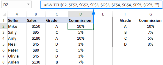
Note. The SWITCH function is only available in Excel 2016 and higher.
Concatenating multiple IF functions in Excel
As mentioned in the previous example, the SWITCH function was introduced only in Excel 2016. To handle similar tasks in older Excel versions, you can combine two or more IF statements by using the Concatenate operator (&) or the CONCATENATE function.
=(IF(C2=»a», 10%, «») & IF(C2=»b», 7%, «») & IF(C2=»c», 5%, «») & IF(C2=»d», 3%, «»))*1
=CONCATENATE(IF(C2=»a», 10%, «»), IF(C2=»b», 7%, «»), IF(C2=»c», 5%, «») & IF(C2=»d», 3%, «»))*1 
As you may have noticed, we multiply the result by 1 in both formulas. It is done to convert a string returned by the Concatenate formula to a number. If your expected output is text, then the multiplication operation is not needed.
You can see that Microsoft Excel provides a handful of good alternatives to nested IF formulas, and hopefully this tutorial has given you some clues on how to leverage them in your worksheets. To have a closer look at the examples discussed in this tutorial, you are welcome to download our sample workbook below. I thank you for reading and hope to see you on our blog next week!
Источник
Excel conditional formatting formulas based on another cell
by Svetlana Cheusheva, updated on February 7, 2023
In this tutorial, we will continue exploring the fascinating world of Excel Conditional Formatting. If you do not feel very comfortable in this area, you may want to look through the previous article first to revive the basics — How to use conditional formatting in Excel.
Today are going to dwell on how to use Excel formulas to format individual cells and entire rows based on the values you specify or based on another cell’s value. This is often considered advanced aerobatics of Excel conditional formatting and once mastered, it will help you push the formats in your spreadsheets far beyond their common uses.
Excel conditional formatting based on another cell value
Excel’s predefined conditional formatting, such as Data Bars, Color Scales and Icon Sets, are mainly purposed to format cells based on their own values. If you want to apply conditional formatting based on another cell or format an entire row based on a single cell’s value, then you will need to use formulas.
So, let’s see how you can make a rule using a formula and after discuss formula examples for specific tasks.
How to create a conditional formatting rule based on formula
To set up a conditional formatting rule based on a formula in any version of Excel 2010 through Excel 365, carry out these steps:
- Select the cells you want to format. You can select one column, several columns or the entire table if you want to apply your conditional format to rows.
Tip. If you plan to add more data in the future and you want the conditional formatting rule to get applied to new entries automatically, you can either:
- Convert a range of cells to a table (Insert tab > Table). In this case, the conditional formatting will be automatically applied to all new rows.
- Select some empty rows below your data, say 100 blank rows.
Tip. Whenever you need to edit a conditional formatting formula, press F2 and then move to the needed place within the formula using the arrow keys. If you try arrowing without pressing F2 , a range will be inserted into the formula rather than just moving the insertion pointer. To add a certain cell reference to the formula, press F2 a second time and then click that cell.
Excel conditional formatting formula examples
Now that you know how to create and apply Excel conditional formatting based on another cell, let’s move on and see how to use various Excel formulas in practice.
Tip. For your Excel conditional formatting formula to work correctly, please always follow these simple rules.
Formulas to compare values (numbers and text)
As you know Microsoft Excel provides a handful of ready-to-use rules to format cells with values greater than, less than or equal to the value you specify (Conditional Formatting >Highlight Cells Rules). However, these rules do not work if you want to conditionally format certain columns or entire rows based on a cell’s value in another column. In this case, you use analogous formulas:
| Condition | Formula example |
|---|---|
| Equal to | =$B2=10 |
| Not equal to | =$B2<>10 |
| Greater than | =$B2>10 |
| Greater than or equal to | =$B2>=10 |
| Less than | =$B2 |
| Less than or equal to | =$B2 |
| Between | =AND($B2>5, $B2 |
The screenshot below shows an example of the Greater than formula that highlights product names in column A if the number of items in stock (column C) is greater than 0. Please pay attention that the formula applies to column A only ($A$2:$A$8). But if you select the whole table (in our case, $A$2:$E$8), this will highlight entire rows based on the value in column C. 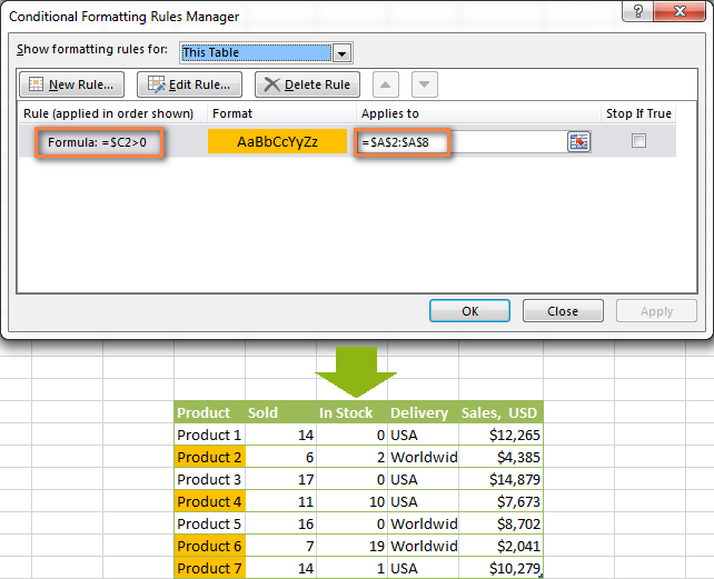
In a similar fashion, you can create a conditional formatting rule to compare values of two cells. For example:
=$A2 — format cells or rows if a value in column A is less than the corresponding value in column B.
=$A2=$B2 — format cells or rows if values in columns A and B are the same.
=$A2<>$B2 — format cells or rows if a value in column A is not the same as in column B.
As you can see in the screenshot below, these formulas work for text values as well as for numbers. 
AND and OR formulas
If you want to format your Excel table based on 2 or more conditions, then use either =AND or =OR function:
| Condition | Formula | Description |
|---|---|---|
| If both conditions are met | =AND($B2 | Formats cells if the value in column B is less than in column C, and if the value in column C is less than in column D. |
| If one of the conditions is met | =OR($B2 | Formats cells if the value in column B is less than in column C, or if the value in column C is less than in column D. |
In the screenshot below, we use the formula =AND($C2>0, $D2=»Worldwide») to change the background color of rows if the number of items in stock (Column C) is greater than 0 and if the product ships worldwide (Column D). Please pay attention that the formula works with text values as well as with numbers. 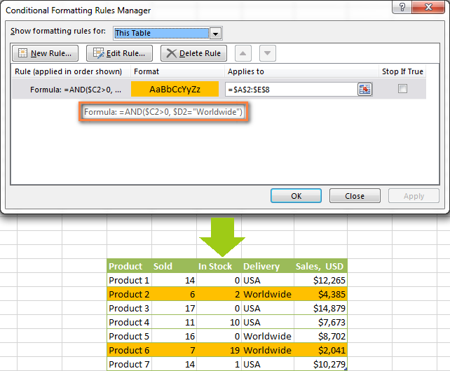
Naturally, you can use two, three or more conditions in your AND and OR formulas. To see how this works in practice, watch Video: Conditional formatting based on another cell.
These are the basic conditional formatting formulas you use in Excel. Now let’s consider a bit more complex but far more interesting examples.
Conditional formatting for empty and non-empty cells
I think everyone knows how to format empty and not empty cells in Excel — you simply create a new rule of the «Format only cells that contain» type and choose either Blanks or No Blanks. ![]()
But what if you want to format cells in a certain column if a corresponding cell in another column is empty or not empty? In this case, you will need to utilize Excel formulas again:
Formula for blanks: =$B2=»» — format selected cells / rows if a corresponding cell in Column B is blank.
Formula for non-blanks: =$B2<>«» — format selected cells / rows if a corresponding cell in Column B is not blank.
Note. The formulas above will work for cells that are «visually» empty or not empty. If you use some Excel function that returns an empty string, e.g. =if(false,»OK», «») , and you don’t want such cells to be treated as blanks, use the following formulas instead =isblank(A1)=true or =isblank(A1)=false to format blank and non-blank cells, respectively.
And here is an example of how you can use the above formulas in practice. Suppose, you have a column (B) which is «Date of Sale» and another column (C) «Delivery«. These 2 columns have a value only if a sale has been made and the item delivered. So, you want the entire row to turn orange when you’ve made a sale; and when an item is delivered, a corresponding row should turn green. To achieve this, you need to create 2 conditional formatting rules with the following formulas:
- Orange rows (a cell in column B is not empty): =$B2<>«»
- Green rows (cells in column B and column C are not empty): =AND($B2<>«», $C2<>«»)
One more thing for you to do is to move the second rule to the top and select the Stop if true check box next to this rule: ![]()
In this particular case, the «Stop if true» option is actually superfluous, and the rule will work with or without it. You may want to check this box just as an extra precaution, in case you add a few other rules in the future that may conflict with any of the existing ones.
Excel formulas to work with text values
If you want to format a certain column(s) when another cell in the same row contains a certain word, you can use a formula discussed in one of the previous examples (like =$D2=»Worldwide»). However, this will only work for exact match.
For partial match, you will need to use either SEARCH (case insensitive) or FIND (case sensitive).
For example, to format selected cells or rows if a corresponding cell in column D contains the word «Worldwide«, use the below formula. This formula will find all such cells, regardless of where the specified text is located in a cell, including «Ships Worldwide«, «Worldwide, except for…«, etc:
If you’d like to shade selected cells or rows if the cell’s content starts with the search text, use this one:
=SEARCH(«Worldwide», $D2)>1 
Excel formulas to highlight duplicates
If your task is to conditionally format cells with duplicate values, you can go with the pre-defined rule available under Conditional formatting > Highlight Cells Rules > Duplicate Values… The following article provides a detailed guidance on how to use this feature: How to automatically highlight duplicates in Excel.
However, in some cases the data looks better if you color selected columns or entire rows when a duplicate values occurs in another column. In this case, you will need to employ an Excel conditional formatting formula again, and this time we will be using the COUNTIF formula. As you know, this Excel function counts the number of cells within a specified range that meet a single criterion.
Highlight duplicates including 1 st occurrences
=COUNTIF($A$2:$A$10,$A2)>1 — this formula finds duplicate values in the specified range in Column A (A2:A10 in our case), including first occurrences.
If you choose to apply the rule to the entire table, the whole rows will get formatted, as you see in the screenshot below. I’ve decided to change a font color in this rule, just for a change : ) 
Highlight duplicates without 1 st occurrences
To ignore the first occurrence and highlight only subsequent duplicate values, use this formula: =COUNTIF($A$2:$A2,$A2)>1 
Highlight consecutive duplicates in Excel
If you’d rather highlight only duplicates on consecutive rows, you can do this in the following way. This method works for any data types: numbers, text values and dates.
- Select the column where you want to highlight duplicates, without the column header.
- Create a conditional formatting rule(s) using these simple formulas:
Rule 1 (blue): =$A1=$A2 — highlights the 2 nd occurrence and all subsequent occurrences, if any.
Rule 2 (green): =$A2=$A3 — highlights the 1 st occurrence.
In the above formulas, A is the column you want to check for dupes, $A1 is the column header, $A2 is the first cell with data.
Important! For the formulas to work correctly, it is essential that Rule 1, which highlights the 2 nd and all subsequent duplicate occurrences, should be the first rule in the list, especially if you are using two different colors. 
Highlight duplicate rows
If you want apply the conditional format when duplicate values occur in two or more columns, you will need to add an extra column to your table in which you concatenate the values from the key columns using a simple formula like this one =A2&B2 . After that you apply a rule using either variation of the COUNTIF formula for duplicates (with or without 1 st occurrences). Naturally, you can hide an additional column after creating the rule. 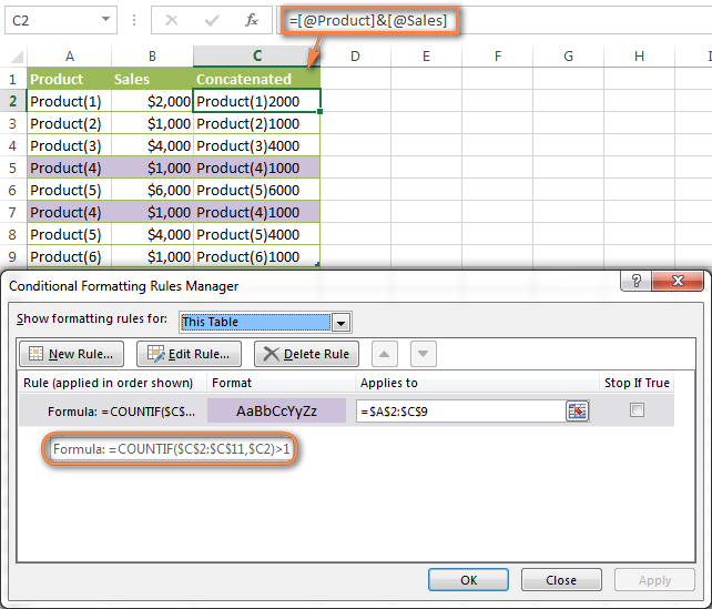
Alternatively, you can use the COUNTIFS function that supports multiple criteria in a single formula. In this case, you won’t need a helper column.
In this example, to highlight duplicate rows with 1st occurrences, create a rule with the following formula:
=COUNTIFS($A$2:$A$11, $A2, $B$2:$B$11, $B2)>1
To highlight duplicate rows without 1st occurrences, use this formula:
=COUNTIFS($A$2:$A2, $A2, $B$2:$B2, $B2)>1
Compare 2 columns for duplicates
One of the most frequent tasks in Excel is to check 2 columns for duplicate values — i.e. find and highlight values that exist in both columns. To do this, you will need to create an Excel conditional formatting rule for each column with a combination of =ISERROR() and =MATCH() functions:
For Column A: =ISERROR(MATCH(A1,$B$1:$B$10000,0))=FALSE
For Column B: =ISERROR(MATCH(B1,$A$1:$A$10000,0))=FALSE
Note. For such conditional formulas to work correctly, it’s very important that you apply the rules to the entire columns, e.g. =$A:$A and =$B:$B .
You can see an example of practical usage in the following screenshot that highlights duplicates in Columns E and F. 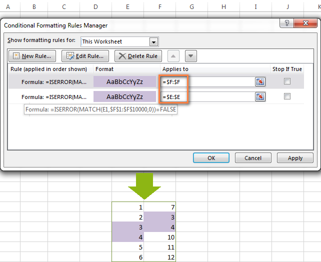
As you can see, Excel conditional formatting formulas cope with dupes pretty well. However, for more complex cases, I would recommend using the Duplicate Remover add-in that is especially designed to find, highlight and remove duplicates in Excel, in one sheet or between two spreadsheets.
Formulas to highlight values above or below average
When you work with several sets of numeric data, the AVERAGE() function may come in handy to format cells whose values are below or above the average in a column.
For example, you can use the formula =$E2 to conditionally format the rows where the sale numbers are below the average, as shown in the screenshot below. If you are looking for the opposite, i.e. to shade the products performing above the average, replace » » in the formula: =$E2>AVERAGE($E$2:$E$8) . 
How to highlight the nearest value in Excel
If I have a set of numbers, is there a way I can use Excel conditional formatting to highlight the number in that set that is closest to zero? This is what one of our blog readers, Jessica, wanted to know. The question is very clear and straightforward, but the answer is a bit too long for the comments sections, that’s why you see a solution here 🙂
Example 1. Find the nearest value, including exact match
In our example, we’ll find and highlight the number that is closest to zero. If the data set contains one or more zeroes, all of them will be highlighted. If there is no 0, then the value closest to it, either positive or negative, will be highlighted.
First off, you need to enter the following formula to any empty cell in your worksheet, you will be able to hide that cell later, if needed. The formula finds the number in a given range that is closest to the number you specify and returns the absolute value of that number (absolute value is the number without its sign):
In the above formula, B2:D13 is your range of cells and 0 is the number for which you want to find the closest match. For example, if you are looking for a value closest to 5, the formula will change to: =MIN(ABS(B2:D13-(5)))
Note. This is an array formula, so you need to press Ctrl + Shift + Enter instead of a simple Enter stroke to complete it.
And now, you create a conditional formatting rule with the following formula, where B3 is the top-right cell in your range and $C$2 in the cell with the above array formula:
Please pay attention to the use of absolute references in the address of the cell containing the array formula ($C$2), because this cell is constant. Also, you need to replace 0 with the number for which you want to highlight the closest match. For example, if we wanted to highlight the value nearest to 5, the formula would change to: =OR(B3=5-$C$2,B3=5+$C$2) 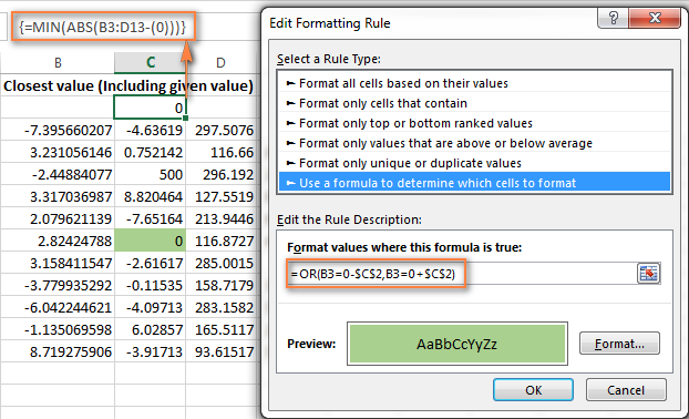
Example 2. Highlight a value closest to the given value, but NOT exact match
In case you do not want to highlight the exact match, you need a different array formula that will find the closest value but ignore the exact match.
For example, the following array formula finds the value closest to 0 in the specified range, but ignores zeroes, if any:
Please remember to press Ctrl + Shift + Enter after you finished typing your array formula.
The conditional formatting formula is the same as in the above example:
However, since our array formula in cell C2 ignores the exact match, the conditional formatting rule ignores zeroes too and highlights the value 0.003 that is the closest match. 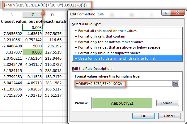
If you want to find the value nearest to some other number in your Excel sheet, just replace «0» with the number you want both in the array and conditional formatting formulas.
I hope the conditional formatting formulas you have learned in this tutorial will help you make sense of whatever project you are working on. If you need more examples, please check out the following articles:
Why isn’t my Excel conditional formatting working correctly?
If your conditional formatting rule is not working as expected, though the formula is apparently correct, do not get upset! Most likely it is not because of some weird bug in Excel conditional formatting, rather due to a tiny mistake, not evident at the first sight. Please try out 6 simple troubleshooting steps below and I’m sure you will get your formula to work:
- Use absolute & relative cell addresses correctly. It’s very difficult to deduce a general rule that will work in 100 per cent of cases. But most often you would use an absolute column (with $) and relative row (without $) in your cell references, e.g. =$A1>1 .
Please keep in mind that the formulas =A1=1 , =$A$1=1 and =A$1=1 will produce different results. If you are not sure which one is correct in your case, you can try all : ) For more information, please see Relative and absolute cell references in Excel conditional formatting.
For example, if your data starts in row 2, you put =A$2=10 to highlight cells with values equal to 10 in all the rows. A common mistake is to always use a reference to the first row (e.g. =A$1=10 ). Please remember, you reference row 1 in the formula only if your table does not have headers and your data really starts in row 1. The most obvious indication of this case is when the rule is working, but formats values not in the rows it should.
And finally, if you’ve tried all the steps but your conditional formatting rule is still not working correctly, drop me a line in comments and we will try to fathom it out together 🙂
In my next article we are going to look into the capabilities of Excel conditional formatting for dates. See you next week and thanks for reading!
Источник
The IF function allows you to make a logical comparison between a value and what you expect by testing for a condition and returning a result if that condition is True or False.
-
=IF(Something is True, then do something, otherwise do something else)
But what if you need to test multiple conditions, where let’s say all conditions need to be True or False (AND), or only one condition needs to be True or False (OR), or if you want to check if a condition does NOT meet your criteria? All 3 functions can be used on their own, but it’s much more common to see them paired with IF functions.
Use the IF function along with AND, OR and NOT to perform multiple evaluations if conditions are True or False.
Syntax
-
IF(AND()) — IF(AND(logical1, [logical2], …), value_if_true, [value_if_false]))
-
IF(OR()) — IF(OR(logical1, [logical2], …), value_if_true, [value_if_false]))
-
IF(NOT()) — IF(NOT(logical1), value_if_true, [value_if_false]))
|
Argument name |
Description |
|
|
logical_test (required) |
The condition you want to test. |
|
|
value_if_true (required) |
The value that you want returned if the result of logical_test is TRUE. |
|
|
value_if_false (optional) |
The value that you want returned if the result of logical_test is FALSE. |
|
Here are overviews of how to structure AND, OR and NOT functions individually. When you combine each one of them with an IF statement, they read like this:
-
AND – =IF(AND(Something is True, Something else is True), Value if True, Value if False)
-
OR – =IF(OR(Something is True, Something else is True), Value if True, Value if False)
-
NOT – =IF(NOT(Something is True), Value if True, Value if False)
Examples
Following are examples of some common nested IF(AND()), IF(OR()) and IF(NOT()) statements. The AND and OR functions can support up to 255 individual conditions, but it’s not good practice to use more than a few because complex, nested formulas can get very difficult to build, test and maintain. The NOT function only takes one condition.

Here are the formulas spelled out according to their logic:
|
Formula |
Description |
|---|---|
|
=IF(AND(A2>0,B2<100),TRUE, FALSE) |
IF A2 (25) is greater than 0, AND B2 (75) is less than 100, then return TRUE, otherwise return FALSE. In this case both conditions are true, so TRUE is returned. |
|
=IF(AND(A3=»Red»,B3=»Green»),TRUE,FALSE) |
If A3 (“Blue”) = “Red”, AND B3 (“Green”) equals “Green” then return TRUE, otherwise return FALSE. In this case only the first condition is true, so FALSE is returned. |
|
=IF(OR(A4>0,B4<50),TRUE, FALSE) |
IF A4 (25) is greater than 0, OR B4 (75) is less than 50, then return TRUE, otherwise return FALSE. In this case, only the first condition is TRUE, but since OR only requires one argument to be true the formula returns TRUE. |
|
=IF(OR(A5=»Red»,B5=»Green»),TRUE,FALSE) |
IF A5 (“Blue”) equals “Red”, OR B5 (“Green”) equals “Green” then return TRUE, otherwise return FALSE. In this case, the second argument is True, so the formula returns TRUE. |
|
=IF(NOT(A6>50),TRUE,FALSE) |
IF A6 (25) is NOT greater than 50, then return TRUE, otherwise return FALSE. In this case 25 is not greater than 50, so the formula returns TRUE. |
|
=IF(NOT(A7=»Red»),TRUE,FALSE) |
IF A7 (“Blue”) is NOT equal to “Red”, then return TRUE, otherwise return FALSE. |
Note that all of the examples have a closing parenthesis after their respective conditions are entered. The remaining True/False arguments are then left as part of the outer IF statement. You can also substitute Text or Numeric values for the TRUE/FALSE values to be returned in the examples.
Here are some examples of using AND, OR and NOT to evaluate dates.

Here are the formulas spelled out according to their logic:
|
Formula |
Description |
|---|---|
|
=IF(A2>B2,TRUE,FALSE) |
IF A2 is greater than B2, return TRUE, otherwise return FALSE. 03/12/14 is greater than 01/01/14, so the formula returns TRUE. |
|
=IF(AND(A3>B2,A3<C2),TRUE,FALSE) |
IF A3 is greater than B2 AND A3 is less than C2, return TRUE, otherwise return FALSE. In this case both arguments are true, so the formula returns TRUE. |
|
=IF(OR(A4>B2,A4<B2+60),TRUE,FALSE) |
IF A4 is greater than B2 OR A4 is less than B2 + 60, return TRUE, otherwise return FALSE. In this case the first argument is true, but the second is false. Since OR only needs one of the arguments to be true, the formula returns TRUE. If you use the Evaluate Formula Wizard from the Formula tab you’ll see how Excel evaluates the formula. |
|
=IF(NOT(A5>B2),TRUE,FALSE) |
IF A5 is not greater than B2, then return TRUE, otherwise return FALSE. In this case, A5 is greater than B2, so the formula returns FALSE. |

Using AND, OR and NOT with Conditional Formatting
You can also use AND, OR and NOT to set Conditional Formatting criteria with the formula option. When you do this you can omit the IF function and use AND, OR and NOT on their own.
From the Home tab, click Conditional Formatting > New Rule. Next, select the “Use a formula to determine which cells to format” option, enter your formula and apply the format of your choice.

Using the earlier Dates example, here is what the formulas would be.

|
Formula |
Description |
|---|---|
|
=A2>B2 |
If A2 is greater than B2, format the cell, otherwise do nothing. |
|
=AND(A3>B2,A3<C2) |
If A3 is greater than B2 AND A3 is less than C2, format the cell, otherwise do nothing. |
|
=OR(A4>B2,A4<B2+60) |
If A4 is greater than B2 OR A4 is less than B2 plus 60 (days), then format the cell, otherwise do nothing. |
|
=NOT(A5>B2) |
If A5 is NOT greater than B2, format the cell, otherwise do nothing. In this case A5 is greater than B2, so the result will return FALSE. If you were to change the formula to =NOT(B2>A5) it would return TRUE and the cell would be formatted. |
Note: A common error is to enter your formula into Conditional Formatting without the equals sign (=). If you do this you’ll see that the Conditional Formatting dialog will add the equals sign and quotes to the formula — =»OR(A4>B2,A4<B2+60)», so you’ll need to remove the quotes before the formula will respond properly.
Need more help?

See also
You can always ask an expert in the Excel Tech Community or get support in the Answers community.
Learn how to use nested functions in a formula
IF function
AND function
OR function
NOT function
Overview of formulas in Excel
How to avoid broken formulas
Detect errors in formulas
Keyboard shortcuts in Excel
Logical functions (reference)
Excel functions (alphabetical)
Excel functions (by category)
This Excel tutorial explains how to use the Excel IF function with syntax and examples.
Description
The Microsoft Excel IF function returns one value if the condition is TRUE, or another value if the condition is FALSE.
The IF function is a built-in function in Excel that is categorized as a Logical Function. It can be used as a worksheet function (WS) in Excel. As a worksheet function, the IF function can be entered as part of a formula in a cell of a worksheet.
![]() Subscribe
Subscribe
If you want to follow along with this tutorial, download the example spreadsheet.
Download Example
Syntax
The syntax for the IF function in Microsoft Excel is:
IF( condition, value_if_true, [value_if_false] )
Parameters or Arguments
- condition
- The value that you want to test.
- value_if_true
- It is the value that is returned if condition evaluates to TRUE.
- value_if_false
- Optional. It is the value that is returned if condition evaluates to FALSE.
Returns
The IF function returns value_if_true when the condition is TRUE.
The IF function returns value_if_false when the condition is FALSE.
The IF function returns FALSE if the value_if_false parameter is omitted and the condition is FALSE.
Example (as Worksheet Function)
Let’s explore how to use the IF function as a worksheet function in Microsoft Excel.
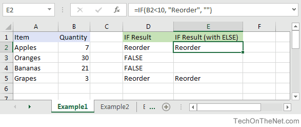
Based on the Excel spreadsheet above, the following IF examples would return:
=IF(B2<10, "Reorder", "")
Result: "Reorder"

=IF(A2="Apples", "Equal", "Not Equal")
Result: "Equal"

=IF(B3>=20, 12, 0)
Result: 12
Combining the IF function with Other Logical Functions
Quite often, you will need to specify more complex conditions when writing your formula in Excel. You can combine the IF function with other logical functions such as AND, OR, etc. Let’s explore this further.
AND function
The IF function can be combined with the AND function to allow you to test for multiple conditions. When using the AND function, all conditions within the AND function must be TRUE for the condition to be met. This comes in very handy in Excel formulas.
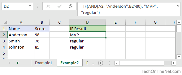
Based on the spreadsheet above, you can combine the IF function with the AND function as follows:
=IF(AND(A2="Anderson",B2>80), "MVP", "regular")
Result: "MVP"

=IF(AND(B2>=80,B2<=100), "Great Score", "Not Bad")
Result: "Great Score"

=IF(AND(B3>=80,B3<=100), "Great Score", "Not Bad")
Result: "Not Bad"

=IF(AND(A2="Anderson",A3="Smith",A4="Johnson"), 100, 50)
Result: 100

=IF(AND(A2="Anderson",A3="Smith",A4="Parker"), 100, 50)
Result: 50
In the examples above, all conditions within the AND function must be TRUE for the condition to be met.
OR function
The IF function can be combined with the OR function to allow you to test for multiple conditions. But in this case, only one or more of the conditions within the OR function needs to be TRUE for the condition to be met.
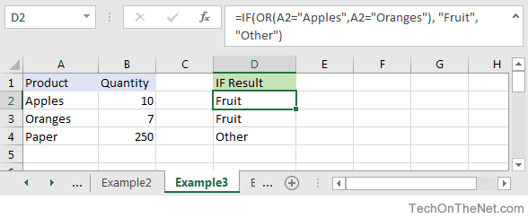
Based on the spreadsheet above, you can combine the IF function with the OR function as follows:
=IF(OR(A2="Apples",A2="Oranges"), "Fruit", "Other")
Result: "Fruit"

=IF(OR(A4="Apples",A4="Oranges"),"Fruit","Other")
Result: "Other"

=IF(OR(A4="Bananas",B4>=100), 999, "N/A")
Result: 999

=IF(OR(A2="Apples",A3="Apples",A4="Apples"), "Fruit", "Other")
Result: "Fruit"
In the examples above, only one of the conditions within the OR function must be TRUE for the condition to be met.
Let’s take a look at one more example that involves ranges of percentages.
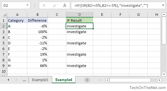
Based on the spreadsheet above, we would have the following formula in cell D2:
=IF(OR(B2>=5%,B2<=-5%),"investigate","")
Result: "investigate"
This IF function would return «investigate» if the value in cell B2 was either below -5% or above 5%. Since -6% is below -5%, it will return «investigate» as the result. We have copied this formula into cells D3 through D9 to show you the results that would be returned.
For example, in cell D3, we would have the following formula:
=IF(OR(B3>=5%,B3<=-5%),"investigate","")
Result: "investigate"
This formula would also return «investigate» but this time, it is because the value in cell B3 is greater than 5%.
Frequently Asked Questions
Question: In Microsoft Excel, I’d like to use the IF function to create the following logic:
if C11>=620, and C10=»F»or»S», and C4<=$1,000,000, and C4<=$500,000, and C7<=85%, and C8<=90%, and C12<=50, and C14<=2, and C15=»OO», and C16=»N», and C19<=48, and C21=»Y», then reference cell A148 on Sheet2. Otherwise, return an empty string.
Answer: The following formula would accomplish what you are trying to do:
=IF(AND(C11>=620, OR(C10="F",C10="S"), C4<=1000000, C4<=500000, C7<=0.85, C8<=0.9, C12<=50, C14<=2, C15="OO", C16="N", C19<=48, C21="Y"), Sheet2!A148, "")
Question: In Microsoft Excel, I’m trying to use the IF function to return 0 if cell A1 is either < 150,000 or > 250,000. Otherwise, it should return A1.
Answer: You can use the OR function to perform an OR condition in the IF function as follows:
=IF(OR(A1<150000,A1>250000),0,A1)
In this example, the formula will return 0 if cell A1 was either less than 150,000 or greater than 250,000. Otherwise, it will return the value in cell A1.
Question: In Microsoft Excel, I’m trying to use the IF function to return 25 if cell A1 > 100 and cell B1 < 200. Otherwise, it should return 0.
Answer: You can use the AND function to perform an AND condition in the IF function as follows:
=IF(AND(A1>100,B1<200),25,0)
In this example, the formula will return 25 if cell A1 is greater than 100 and cell B1 is less than 200. Otherwise, it will return 0.
Question: In Microsoft Excel, I need to write a formula that works this way:
IF (cell A1) is less than 20, then times it by 1,
IF it is greater than or equal to 20 but less than 50, then times it by 2
IF its is greater than or equal to 50 and less than 100, then times it by 3
And if it is great or equal to than 100, then times it by 4
Answer: You can write a nested IF statement to handle this. For example:
=IF(A1<20, A1*1, IF(A1<50, A1*2, IF(A1<100, A1*3, A1*4)))
Question: In Microsoft Excel, I need a formula in cell C5 that does the following:
IF A1+B1 <= 4, return $20
IF A1+B1 > 4 but <= 9, return $35
IF A1+B1 > 9 but <= 14, return $50
IF A1+B1 >= 15, return $75
Answer: In cell C5, you can write a nested IF statement that uses the AND function as follows:
=IF((A1+B1)<=4,20,IF(AND((A1+B1)>4,(A1+B1)<=9),35,IF(AND((A1+B1)>9,(A1+B1)<=14),50,75)))
Question: In Microsoft Excel, I need a formula that does the following:
IF the value in cell A1 is BLANK, then return «BLANK»
IF the value in cell A1 is TEXT, then return «TEXT»
IF the value in cell A1 is NUMERIC, then return «NUM»
Answer: You can write a nested IF statement that uses the ISBLANK function, the ISTEXT function, and the ISNUMBER function as follows:
=IF(ISBLANK(A1)=TRUE,"BLANK",IF(ISTEXT(A1)=TRUE,"TEXT",IF(ISNUMBER(A1)=TRUE,"NUM","")))
Question: In Microsoft Excel, I want to write a formula for the following logic:
IF R1<0.3 AND R2<0.3 AND R3<0.42 THEN «OK» OTHERWISE «NOT OK»
Answer: You can write an IF statement that uses the AND function as follows:
=IF(AND(R1<0.3,R2<0.3,R3<0.42),"OK","NOT OK")
Question: In Microsoft Excel, I need a formula for the following:
IF cell A1= PRADIP then value will be 100
IF cell A1= PRAVIN then value will be 200
IF cell A1= PARTHA then value will be 300
IF cell A1= PAVAN then value will be 400
Answer: You can write an IF statement as follows:
=IF(A1="PRADIP",100,IF(A1="PRAVIN",200,IF(A1="PARTHA",300,IF(A1="PAVAN",400,""))))
Question: In Microsoft Excel, I want to calculate following using an «if» formula:
if A1<100,000 then A1*.1% but minimum 25
and if A1>1,000,000 then A1*.01% but maximum 5000
Answer: You can write a nested IF statement that uses the MAX function and the MIN function as follows:
=IF(A1<100000,MAX(25,A1*0.1%),IF(A1>1000000,MIN(5000,A1*0.01%),""))
Question: In Microsoft Excel, I am trying to create an IF statement that will repopulate the data from a particular cell if the data from the formula in the current cell equals 0. Below is my attempt at creating an IF statement that would populate the data; however, I was unsuccessful.
=IF(IF(ISERROR(M24+((L24-S24)/AA24)),"0",M24+((L24-S24)/AA24)))=0,L24)
The initial part of the formula calculates the EAC (Estimate At completion = AC+(BAC-EV)/CPI); however if the current EV (Earned Value) is zero, the EAC will equal zero. IF the outcome is zero, I would like the BAC (Budget At Completion), currently recorded in another cell (L24), to be repopulated in the current cell as the EAC.
Answer: You can write an IF statement that uses the OR function and the ISERROR function as follows:
=IF(OR(S24=0,ISERROR(M24+((L24-S24)/AA24))),L24,M24+((L24-S24)/AA24))
Question: I have been looking at your Excel IF, AND and OR sections and found this very helpful, however I cannot find the right way to write a formula to express if C2 is either 1,2,3,4,5,6,7,8,9 and F2 is F and F3 is either D,F,B,L,R,C then give a value of 1 if not then 0. I have tried many formulas but just can’t get it right, can you help please?
Answer: You can write an IF statement that uses the AND function and the OR function as follows:
=IF(AND(C2>=1,C2<=9, F2="F",OR(F3="D",F3="F",F3="B",F3="L",F3="R",F3="C")),1,0)
Question:In Excel, I have a roadspeed of a car in m/s in cell A1 and a drop down menu of different units in C1 (which unclude mph and kmh). I have used the following IF function in B1 to convert the number to the unit selected from the dropdown box:
=IF(C1="mph","=A1*2.23693629",IF(C1="kmh","A1*3.6"))
However say if kmh was selected B1 literally just shows A1*3.6 and does not actually calculate it. Is there away to get it to calculate it instead of just showing the text message?
Answer: You are very close with your formula. Because you are performing mathematical operations (such as A1*2.23693629 and A1*3.6), you do not need to surround the mathematical formulas in quotes. Quotes are necessary when you are evaluating strings, not performing math.
Try the following:
=IF(C1="mph",A1*2.23693629,IF(C1="kmh",A1*3.6))
Question:For an IF statement in Excel, I want to combine text and a value.
For example, I want to put an equation for work hours and pay. IF I am paid more than I should be, I want it to read how many hours I owe my boss. But if I work more than I am paid for, I want it to read what my boss owes me (hours*Pay per Hour).
I tried the following:
=IF(A2<0,"I owe boss" abs(A2) "Hours","Boss owes me" abs(A2)*15 "dollars")
Is it possible or do I have to do it in 2 separate cells? (one for text and one for the value)
Answer: There are two ways that you can concatenate text and values. The first is by using the & character to concatenate:
=IF(A2<0,"I owe boss " & ABS(A2) & " Hours","Boss owes me " & ABS(A2)*15 & " dollars")
Or the second method is to use the CONCATENATE function:
=IF(A2<0,CONCATENATE("I owe boss ", ABS(A2)," Hours"), CONCATENATE("Boss owes me ", ABS(A2)*15, " dollars"))
Question:I have Excel 2000. IF cell A2 is greater than or equal to 0 then add to C1. IF cell B2 is greater than or equal to 0 then subtract from C1. IF both A2 and B2 are blank then equals C1. Can you help me with the IF function on this one?
Answer: You can write a nested IF statement that uses the AND function and the ISBLANK function as follows:
=IF(AND(ISBLANK(A2)=FALSE,A2>=0),C1+A2, IF(AND(ISBLANK(B2)=FALSE,B2>=0),C1-B2, IF(AND(ISBLANK(A2)=TRUE, ISBLANK(B2)=TRUE),C1,"")))
Question:How would I write this equation in Excel? IF D12<=0 then D12*L12, IF D12 is > 0 but <=600 then D12*F12, IF D12 is >600 then ((600*F12)+((D12-600)*E12))
Answer: You can write a nested IF statement as follows:
=IF(D12<=0,D12*L12,IF(D12>600,((600*F12)+((D12-600)*E12)),D12*F12))
Question:In Excel, I have this formula currently:
=IF(OR(A1>=40, B1>=40, C1>=40), "20", (A1+B1+C1)-20)
If one of my salesman does sale for $40-$49, then his commission is $20; however if his/her sale is less (for example $35) then the commission is that amount minus $20 ($35-$20=$15). I have 3 columns that are needed based on the type of sale. Only one column per row will be needed. The problem is that, when left blank, the total in the formula cell is -20. I need help setting up this formula so that when the 3 columns are left blank, the cell with the formula is left blank as well.
Answer: Using the AND function and the ISBLANK function, you can write your IF statement as follows:
=IF(AND(ISBLANK(A1),ISBLANK(B1),ISBLANK(C1)),"",IF(OR(A1>40, B1>40, C1>40), "20", (A1+B1+C1)-20))
In this formula, we are using the ISBLANK function to check if all 3 cells A1, B1, and C1 are blank, and if they are return a blank value («»). Then the rest is the formula that you originally wrote.
Question:In Excel, I need to create a simple booking and and out system, that shows a date out and a date back
«A1» = allows person to input date booked out
«A2» =allows person to input date booked back in
«A3″= shows status of product, eg, booked out, overdue return etc.
I can automate A3 with the following IF function:
=IF(ISBLANK(A2),"booked out","returned")
But what I cant get to work is if the product is out for 10 days or more, I would like the cell to say «send email»
Can you assist?
Answer: Using the TODAY function and adding an additional IF function, you can write your formula as follows:
=IF(ISBLANK(A2),IF(TODAY()-A1>10,"send email","booked out"),"returned")
Question:Using Microsoft Excel, I need a formula in cell U2 that does the following:
IF the date in E2<=12/31/2010, return T2*0.75
IF the date in E2>12/31/2010 but <=12/31/2011, return T2*0.5
IF the date in E2>12/31/2011, return T2*0
I tried using the following formula, but it gives me «#VALUE!»
=IF(E2<=DATE(2010,12,31),T2*0.75), IF(AND(E2>DATE(2010,12,31),E2<=DATE(2011,12,31)),T2*0.5,T2*0)
Can someone please help? Thanks.
Answer: You were very close…you just need to adjust your parentheses as follows:
=IF(E2<=DATE(2010,12,31),T2*0.75, IF(AND(E2>DATE(2010,12,31),E2<=DATE(2011,12,31)),T2*0.5,T2*0))
Question:In Excel, I would like to add 60 days if grade is ‘A’, 45 days if grade is ‘B’ and 30 days if grade is ‘C’. It would roughly look something like this, but I’m struggling with commas, brackets, etc.
(IF C5=A)=DATE(YEAR(B5)+0,MONTH(B5)+0,DAY(B5)+60),
(IF C5=B)=DATE(YEAR(B5)+0,MONTH(B5)+0,DAY(B5)+45),
(IF C5=C)=DATE(YEAR(B5)+0,MONTH(B5)+0,DAY(B5)+30)
Answer:You should be able to achieve your date calculations with the following formula:
=IF(C5="A",B5+60,IF(C5="B",B5+45,IF(C5="C",B5+30)))
Question:In Excel, I am trying to write a function and can’t seem to figure it out. Could you help?
IF D3 is < 31, then 1.51
IF D3 is between 31-90, then 3.40
IF D3 is between 91-120, then 4.60
IF D3 is > 121, then 5.44
Answer:You can write your formula as follows:
=IF(D3>121,5.44,IF(D3>=91,4.6,IF(D3>=31,3.4,1.51)))
Question:I would like ask a question regarding the IF statement. How would I write in Excel this problem?
I have to check if cell A1 is empty and if not, check if the value is less than equal to 5. Then multiply the amount entered in cell A1 by .60. The answer will be displayed on Cell A2.
Answer:You can write your formula in cell A2 using the IF function and ISBLANK function as follows:
=IF(AND(ISBLANK(A1)=FALSE,A1<=5),A1*0.6,"")
Question:In Excel, I’m trying to nest an OR command and I can’t find the proper way to write it. I want the spreadsheet to do the following:
If D6 equals «HOUSE» and C6 equals either «MOUSE» or «CAT», I want to return the value in cell B6. Otherwise, the formula should return the value «BLANK».
I tried the following:
=IF((D6="HOUSE")*(C6="MOUSE")*OR(C6="CAT"));B6;"BLANK")
If I only ask for HOUSE and MOUSE or HOUSE and CAT, it works, but as soon as I ask for MOUSE OR CAT, it doesn’t work.
Answer:You can write your formula using the AND function and OR function as follows:
=IF(AND(D6="HOUSE",OR(C6="MOUSE",C6="CAT")),B6,"BLANK")
This will return the value in B6 if D6 equals «HOUSE» and C6 equals either «MOUSE» or «CAT». If those conditions are not met, the formula will return the text value of «BLANK».
Question:In Microsoft Excel, I’m trying to write the following formula:
If cell A1 equals «jaipur», «udaipur» or «jodhpur», then cell A2 should display «rajasthan»
If cell A1 equals «bangalore», «mysore» or «belgum», then cell A2 should display «karnataka»
Please help.
Answer:You can write your formula using the OR function as follows:
=IF(OR(A1="jaipur",A1="udaipur",A1="jodhpur"),"rajasthan", IF(OR(A1="bangalore",A1="mysore",A1="belgum"),"karnataka"))
This will return «rajasthan» if A1 equals either «jaipur», «udaipur» or «jodhpur» and it will return «karnataka» if A1 equals either «bangalore», «mysore» or «belgum».
Question:In Microsoft Excel I’m trying to achieve the following with IF function:
If a value in any cell in column F is «food» then add the value of its corresponding cell in column G (eg a corresponding cell for F3 is G3). The IF function is performed in another cell altogether. I can do it for a single pair of cells but I don’t know how to do it for an entire column. Could you help?
At the moment, I’ve got this:
=IF(F3="food"; G3; 0)
Answer:This formula can be created using the SUMIF formula instead of using the IF function:
=SUMIF(F1:F10,"=food",G1:G10)
This will evaluate the first 10 rows of data in your spreadsheet. You may need to adjust the ranges accordingly.
I notice that you separate your parameters with semi-colons, so you might need to replace the commas in the formula above with semi-colons.
Question:I’m looking for an Exel formula that says:
If F3 is «H» and E3 is «H», return 1
If F3 is «A» and E3 is «A», return 2
If F3 is «d» and E3 is «d», return 3
Appreciate if you can help.
Answer:This Excel formula can be created using the AND formula in combination with the IF function:
=IF(AND(F3="H",E3="H"),1,IF(AND(F3="A",E3="A"),2,IF(AND(F3="d",E3="d"),3,"")))
We’ve defaulted the formula to return a blank if none of the conditions above are met.
Question:I am trying to get Excel to check different boxes and check if there is text/numbers listed in the cells and then spit out «Complete» if all 5 Boxes have text/Numbers or «Not Complete» if one or more is empty. This is what I have so far and it doesn’t work.
=IF(OR(ISBLANK(J2),ISBLANK(M2),ISBLANK(R2),ISBLANK (AA2),ISBLANK (AB2)),"Not Complete","")
Answer:First, you are correct in using the ISBLANK function, however, you have a space between ISBLANK and (AA2), as well as ISBLANK and (AB2). This might seem insignificant, but Excel can be very picky and will return a #NAME? error. So first you need to eliminate those spaces.
Next, you need to change the ELSE condition of your IF function to return «Complete».
You should be able to modify your formula as follows:
=IF(OR(ISBLANK(J2),ISBLANK(M2),ISBLANK(R2),ISBLANK(AA2),ISBLANK(AB2)), "Not Complete", "Complete")
Now if any of the cell J2, M2, R2, AA2, or AB2 are blank, the formula will return «Not Complete». If all 5 cells have a value, the formula will return «Complete».
Question:I’m very new to the Excel world, and I’m trying to figure out how to set up the proper formula for an If/then cell.
What I’m trying for is:
If B2’s value is 1 to 5, then multiply E2 by .77
If B2’s value is 6 to 10, then multiply E2 by .735
If B2’s value is 11 to 19, then multiply E2 by .7
If B2’s value is 20 to 29, then multiply E2 by .675
If B2’s value is 30 to 39, then multiply E2 by .65
I’ve tried a few different things thinking I was on the right track based on the IF, and AND function tutorials here, but I can’t seem to get it right.
Answer:To write your IF formula, you need to nest multiple IF functions together in combination with the AND function.
The following formula should work for what you are trying to do:
=IF(AND(B2>=1, B2<=5), E2*0.77, IF(AND(B2>=6, B2<=10), E2*0.735, IF(AND(B2>=11, B2<=19), E2*0.7, IF(AND(B2>=20, B2<=29), E2*0.675, IF(AND(B2>=30, B2<=39), E2*0.65,"")))))
As one final component of your formula, you need to decide what to do when none of the conditions are met. In this example, we have returned «» when the value in B2 does not meet any of the IF conditions above.
Question:Here is the Excel formula that has me between a rock and a hard place.
If E45 <= 50, return 44.55
If E45 > 50 and E45 < 100, return 42
If E45 >=200, return 39.6
Again thank you very much.
Answer:You should be able to write this Excel formula using a combination of the IF function and the AND function.
The following formula should work:
=IF(E45<=50, 44.55, IF(AND(E45>50, E45<100), 42, IF(E45>=200, 39.6, "")))
Please note that if none of the conditions are met, the Excel formula will return «» as the result.
Question:I have a nesting OR function problem:
My nonworking formula is:
=IF(C9=1,K9/J7,IF(C9=2,K9/J7,IF(C9=3,K9/L7,IF(C9=4,0,K9/N7))))
In Cell C9, I can have an input of 1, 2, 3, 4 or 0. The problem is on how to write the «or» condition when a «4 or 0» exists in Column C. If the «4 or 0» conditions exists in Column C I want Column K divided by Column N and the answer to be placed in Column M and associated row
Answer:You should be able to use the OR function within your IF function to test for C9=4 OR C9=0 as follows:
=IF(C9=1,K9/J7,IF(C9=2,K9/J7,IF(C9=3,K9/L7,IF(OR(C9=4,C9=0),K9/N7))))
This formula will return K9/N7 if cell C9 is either 4 or 0.
Question:In Excel, I am trying to create a formula that will show the following:
If column B = Ross and column C = 8 then in cell AB of that row I want it to show 2013, If column B = Block and column C = 9 then in cell AB of that row I want it to show 2012.
Answer:You can create your Excel formula using nested IF functions with the AND function.
=IF(AND(B1="Ross",C1=8),2013,IF(AND(B1="Block",C1=9),2012,""))
This formula will return 2013 as a numeric value if B1 is «Ross» and C1 is 8, or 2012 as a numeric value if B1 is «Block» and C1 is 9. Otherwise, it will return blank, as denoted by «».
Question:In Excel, I really have a problem looking for the right formula to express the following:
If B1=0, C1 is equal to A1/2
If B1=1, C1 is equal to A1/2 times 20%
If D1=1, C1 is equal to A1/2-5
I’ve been trying to look for any same expressions in your site. Please help me fix this.
Answer:In cell C1, you can use the following Excel formula with 3 nested IF functions:
=IF(B1=0,A1/2, IF(B1=1,(A1/2)*0.2, IF(D1=1,(A1/2)-5,"")))
Please note that if none of the conditions are met, the Excel formula will return «» as the result.
Question:In Excel, I need the answer for an IF THEN statement which compares column A and B and has an «OR condition» for column C. My problem is I want column D to return yes if A1 and B1 are >=3 or C1 is >=1.
Answer:You can create your Excel IF formula as follows:
=IF(OR(AND(A1>=3,B1>=3),C1>=1),"yes","")
Please note that if none of the conditions are met, the Excel formula will return «» as the result.
Question:In Excel, what have I done wrong with this formula?
=IF(OR(ISBLANK(C9),ISBLANK(B9)),"",IF(ISBLANK(C9),D9-TODAY(), "Reactivated"))
I want to make an event that if B9 and C9 is empty, the value would be empty. If only C9 is empty, then the output would be the remaining days left between the two dates, and if the two cells are not empty, the output should be the string ‘Reactivated’.
The problem with this code is that IF(ISBLANK(C9),D9-TODAY() is not working.
Answer:First of all, you might want to replace your OR function with the AND function, so that your Excel IF formula looks like this:
=IF(AND(ISBLANK(C9),ISBLANK(B9)),"",IF(ISBLANK(C9),D9-TODAY(),"Reactivated"))
Next, make sure that you don’t have any abnormal formatting in the cell that contains the results. To be safe, right click on the cell that contains the formula and choose Format Cells from the popup menu. When the Format Cells window appears, select the Number tab. Choose General as the format and click on the OK button.
Question:I was wondering if you could tell me what I am doing wrong.
Here are the instructions:
A customer is eligible for a discount if the customer’s 2016 sales greater than or equal to 100000 OR if the customers First Order was placed in 2016.
If the customer qualifies for a discount, return a value of Y
If the customer does not qualify for a discount, return a value of N.
Here is the formula I’ve entered:
=IF(OR([2014 Sales]=0,[2015 Sales]=0,[2016 Sales]>=100000),"Y","N")
I only have 2 cells wrong. Can you help me please? I am very lost and confused.
Answer:You are very close with your IF formula, however, it looks like you need to add the AND function to your formula as follows:
=IF(OR([2016 Sales]>=100000,AND([2014 Sales]=0,[2015 Sales]=0),C8>=100000),"Y","N")
This formula should return Y if 2016 sales are greater than or equal to 100000, or if both 2014 sales and 2015 sales are 0. Otherwise, the formula will return N. You will also notice that we switched the order of your conditions in the formula so that it is easier to understand the formula based on your instructions above.
Question:Could you please help me? I need to use «OR» on my formula but I can’t get it to work. This is what I’ve tried:
=IF(C6>=0<=150,150000,IF(C6>=151<=160,158400))
Here is what I need the formula to do:
IF C6 IS >=0 OR <=150 THEN ASSIGN $150000
IF C6 IS >=151 OR <=160 THEN ASSIGN $158400
Answer:You should be able to use the AND function within your IF function as follows:
=IF(AND(ISBLANK(C6)=FALSE,C6>=0,C6<=150),150000,IF(AND(C6>=151,C6<=160),158400,""))
Notice that we first use the ISBLANK function to test C6 to make sure that it is not blank. This is because if C6 if blank, it will evalulate to greater than 0 and thus return 150000. To avoid this, we include ISBLANK(C6)=FALSE as one of the conditions in addition to C6>=0 and C6<=150. That way, you won’t return any false results if C6 is blank.
Question:I am having a problem with a formula, I want it to be IF E5=N then do the first formula, else do the second formula. Excel recognizes the =IF(logical_test,value_if_TRUE,value_if_FALSE) but doesn’t like the formula below:
=IF(e5="N",((AND(AH5-AG5<456, AH5-S5<822)), "Compliant", "not Compliant"),((AH5-S5<822), "Compliant", "not Compliant"))
Any help would be greatly appreciated.
Answer:To have the first formula executed when E5=N and then second formula executed when E5<>N, you will need to nest 2 additional IF functions within the main IF function as follows:
=IF(E5="N", IF((AND(AH5-AG5<456, AH5-S5<822)), "Compliant", "not Compliant"), IF((AH5-S5<822), "Compliant", "not Compliant"))
If E5=»N», the first nested IF function will be executed:
IF((AND(AH5-AG5<456, AH5-S5<822)), "Compliant", "not Compliant")
Otherwise,the second nested IF function will be executed:
IF((AH5-S5<822), "Compliant", "not Compliant"))
Question:I need to write a formula based on the following logic:
There is a maximum discount allowed of £1000 if the capital sum is less that £43000 and a lower discount of £500 if the capital sum is above £43000. So the formula should return either £500 or £1000 in the cell but the £43000 is made up of two numbers, say for e.g. £42750+350 and if the second number is less than the allowed discount, the actual lower value is returned — in this case the £500 or £1000 becomes £350. Or as another e.g. £42000+750 returns £750.
So on my spreadsheet, in this second e.g. I would have A1= £42000, A2=750, A3=A1+A2, A4=the formula with the changing discount, in this case £750.
How can I write this formula?
Answer:In cell A4, you can calculate the correct discount using the IF function and the MIN function as follows:
=IF(A3<43000, MIN(A2,1000), MIN(A2,500))
If A3 is less than 43000, the formula will return the lower value of A2 and 1000. Otherwise, it will return the lower value of A2 and 500.
Question: I have a list of sizes in column A with sizes 100, 200, 300, 400, 500, 600. Then I have another column B, with sizes of my products, and it is random, for example, 318, 445, 527. What I’m trying to create is for a value of 318 in column B, I need to return 400 for that product. If the value in column B is 445, then I should return 500 and so on, as long sizes in column A must be BIGGER to the NEAREST size to column B.
Any idea how to create this function?
Answer:If your sizes are in increments of 100, you can create this function by taking the value in column B, dividing by 100, rounding up to the nearest integer, and then multiplying by 100.
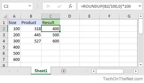
For example in cell C2, you can use the IF function and the ROUNDUP function as follows:
=ROUNDUP(B2/100,0)*100
This will return the correct value of 400 for a value of 318 in cell B2. Just copy this formula to cell C3, C4 and so on.
![]()
Download Article
![]()
Download Article
Are you new to Microsoft Excel and need to work on a spreadsheet? Excel is so overrun with useful and complicated features that it might seem impossible for a beginner to learn. But don’t worry—once you learn a few basic tricks, you’ll be entering, manipulating, calculating, and graphing data in no time! This wikiHow tutorial will introduce you to the most important features and functions you’ll need to know when starting out with Excel, from entering and sorting basic data to writing your first formulas.
Things You Should Know
- Use Quick Analysis in Excel to perform quick calculations and create helpful graphs without any prior Excel knowledge.
- Adding your data to a table makes it easy to sort and filter data by your preferred criteria.
- Even if you’re not a math person, you can use basic Excel math functions to add, subtract, find averages and more in seconds.
-

1
Create or open a workbook. When people refer to «Excel files,» they are referring to workbooks, which are files that contain one or more sheets of data on individual tabs. Each tab is called a worksheet or spreadsheet, both of which are used interchangeably. When you open Excel, you’ll be prompted to open or create a workbook.
- To start from scratch, click Blank workbook. Otherwise, you can open an existing workbook or create a new one from one of Excel’s helpful templates, such as those designed for budgeting.
-
2
Explore the worksheet. When you create a new blank workbook, you’ll have a single worksheet called Sheet1 (you’ll see that on the tab at the bottom) that contains a grid for your data. Worksheets are made of individual cells that are organized into columns and rows.
- Columns are vertical and labeled with letters, which appear above each column.
- Rows are horizontal and are labeled by numbers, which you’ll see running along the left side of the worksheet.
- Every cell has an address which contains its column letter and row number. For example, the top-left cell in your worksheet’s address is A1 because it’s in column A, row 1.
- A workbook can have multiple worksheets, all containing different sets of data. Each worksheet in your workbook has a name—you can rename a worksheet by right-clicking its tab and selecting Rename.
- To add another worksheet, just click the + next to the worksheet tab(s).
Advertisement
-
3
Save your workbook. Once you save your workbook once, Excel will automatically save any changes you make by default.[1]
This prevents you from accidentally losing data.- Click the File menu and select Save As.
- Choose a location to save the file, such as on your computer or in OneDrive.
- Type a name for your workbook. All workbooks will automatically inherit the the .XLSX file extension.
- Click Save.


Advertisement
-
1
Click a cell to select it. When you click a cell, it will highlight to indicate that it’s selected.
- When you type something into a cell, the input text is called a value. Entering data into Excel is as simple as typing values into each cell.
- When entering data, the first row of your worksheet (e.g., A1, B1, C1) is typically used as headers for each column. This is helpful when creating graphs or tables which require labels.
- For example, if you’re adding a list of dates in column A, you might click cell A1 and type Date into the cell as the column header.
-
2
Type a word or number into the cell. As you’re typing, you’ll see the letters and/or numbers appear in the cell, as well as in the formula bar at the top of the worksheet.
- When you start practicing more advanced Excel features like creating formulas, this bar will come in handy.
- You can also copy and paste text from other applications into your worksheet, tables from PDFs and the web.
-
3
Press ↵ Enter or ⏎ Return. This enters the data into the cell and moves to the next cell in the column.
-
4
Automatically fill columns based on existing data. Let’s say you want to make a list of consecutive dates or numbers. Or what if you want to fill a column with many of the same values that follow a pattern? As long as Excel can recognize some sort of pattern in your data, such as a particular order, you can use Autofill to automatically populate data into the rest of your column. Here’s a trick to see it in action.
- In a blank column, type 1 into the first cell, 2 into the second cell, and then 3 into the third cell.
- Hover your mouse cursor over the bottom-right corner of the last cell in your series—it will turn to a crosshair.
- Click and drag the crosshair down the column, then release the mouse button once you’ve gone down as far as you like. By default, this will fill the remaining cells with the value of the selected cell—at this point, you’ll probably have something like 1, 2, 3, 3, 3, 3, 3, 3.
- Click the small icon at the bottom-right corner of the filled data to open AutoFill options, and select Fill Series to automatically detect the series or pattern. Now you’ll have a list of consecutive numbers. Try this cool feature out with different patterns!
- Once you get the hang of AutoFill, you’ll have to try flash fill, which you can use to join two columns of data into a single merged column.
-
5
Adjust the column sizes so you can see all of the values. Sometimes typing long values into a cell hides the value and displays hash symbols ### instead of what you’ve typed. If you want to be able to see everything, you can snap the cell contents to the width of the widest cell. For example, let’s say we have some long values in column B:
- To expand the contents of column B, hover the cursor over the dividing line between the B and C at the top of the worksheet—once your cursor is right on the line, it will turn to two arrows pointing in either direction.[2]
- Click and drag the separator until the column is wide enough to accommodate your data, or just double-click the separator to instantly snap the column to the size of the widest value.
- To expand the contents of column B, hover the cursor over the dividing line between the B and C at the top of the worksheet—once your cursor is right on the line, it will turn to two arrows pointing in either direction.[2]
-
6
Wrap text in a cell. If your longer values are now awkwardly long, you can enable text wrapping in one or more cells. Just click a cell (or drag the mouse to select multiple cells), click the Home tab, and then click Wrap Text on the toolbar.
-
7
Edit a cell value. If you need to make a change to a cell, you can double-click the cell to activate the cursor, and then make any changes you need. When you’re finished, just press Enter or Return again.
- To delete the contents of a cell, click the cell once and press delete on your keyboard.
-
8
Apply styles to your data. Whether you want to highlight certain values with color so they stand out or just want to make your data look pretty, changing the colors of cells and their containing values is easy—especially if you’re used to Microsoft Word:
- Select a cell, column, row, or multiple cells at once.
- On the Home tab, click Cell Styles if you’d like to quickly apply quick color styles.
- If you’d rather use more custom options, right-click the selected cell(s) and select Format Cells. Then, use the colors on the Fill tab to customize the cell’s background, or the colors on the Font tab for value colors.
-
9
Apply number formatting to cells containing numbers. If you have data that contains numbers such as prices, measurements, dates, or times, you can apply number formatting to the data so it will display consistently.[3]
By default, the number format is General, which means numbers display exactly as you type them.- Select the cell you want to format. If you’re working with an entire column or row, you can just click the column letter or row number to select the whole thing.
- On the Home tab, click the drop-down menu at the top-center—it’ll say General by default, unless you selected cells that Excel recognizes as a different type of number like Currency or Time.
- Choose one of the formatting options in the list, such as Short Date or Percentage, or click More Number Formats at the bottom to expand all options (we recommend this!).
- If you selected More Number Formats, the Format Cells dialog will expand to the Number tab, where you’ll see several categories for number types.
- Select a category, such as Currency if working with money, or Date if working with dates. Then, choose your preferences, such as a currency symbol and/or decimal places.
- Click OK to apply your formatting.


Advertisement
-
1
Select all of the data you’ve entered so far. Adding your data to a table is the easiest way to work with and analyze data.[4]
Start by highlighting the values you’ve entered so far, including your column headers. Tables also make it easy to sort and filter your data based on values.- Tables traditionally apply different or alternating colors to every other row for easy viewing. Many table options also add borders between cells and/or columns and rows.
-
2
Click Format as Table. You’ll see this at the top-center part of the Home tab.[5]
-
3
Select a table style. Choose any of Excel’s default table styles to get started. You’ll see a small window titled «Create Table» once selected.
- Once you get the hang of tables, you can return here to customize your table further by selecting New Table Style.
-
4
Make sure «My table has headers» is selected and click OK. This tells Excel to turn your column headers into drop-down menus that you can easily sort and filter. Once you click OK, you’ll see that your data now has a color scheme and drop-down menus.
-
5
Click the drop-down menu at the top of a column. Now you’ll see options for sorting that column, as well as several options for filtering all of your data based on its values.
-
6
Choose which data to display based on values in this column. The simplest way to do this is to uncheck the values you don’t want to display—if you uncheck a particular date, for example, you’ll prevent rows that contain the selected date in from appearing in your data. You can also use Text Filters or Number Filters, depending on the type of data in the column:
- If you chose a numerical column, select Number Filters, then choose an option like Greater Than… or Does Not Equal to be extra specific about which values to hide.
- For text columns, you can choose Text Filters, where you can specify things like Begins with or Contains.
- You can also filter by cell color.
-
7
Click OK. Your data is now filtered based on your selections. You’ll also see a small funnel icon in the drop-down menu, which indicates that the data is filtering out certain values.
- To unfilter your data, click the funnel icon, click Clear filter from (column name), and then click OK.
- You can also filter columns that aren’t in tables. Just select a column and click Filter on the Data tab to add a drop-down to that column.
-
8
Sort your data in ascending or descending order. Click the drop-down arrow at the top of a column to view sorting options—these allow you to sort all of your data in order based on the current column.
- If you’re working with numbers, click Smallest to Largest to sort in ascending order, or Largest to Smallest for descending order.[6]
- If you’re working with text values, Sort A to Z will sort in ascending order, while Sort Z to A will sort in reverse.
- When it comes to sorting dates and times, Sort Oldest to Newest will sort with the earliest date at the top and the oldest date at the bottom, and Newest to Oldest displays the dates in descending order.
- When you sort a column, all other columns in the table adjust based on the sort.
- If you’re working with numbers, click Smallest to Largest to sort in ascending order, or Largest to Smallest for descending order.[6]


Advertisement
-
1
Select the data in your worksheet. Excel’s Quick Analysis feature is the easiest way to perform basic calculations (including totals, averages, and counts) and create meaningful tables or graphs without the need for advanced Excel knowledge.[7]
Use your mouse to select your data (including your column headers) to get started. -
2
Click the Quick Analysis icon. This is the small icon that pops up at the bottom-right corner of your selection. It looks like a window with some colored lines.
-
3
Select an analysis type. You’ll see several tabs running along the top of the window, each of which gives you different option for visualizing your data:
- For math calculations, click the Totals tab, where you can select Sum, Average, Count, %Total, or Running Total. You’ll be able to choose whether to display the results at the bottom of each column or to the right.
- To create a chart, click the Charts tab, then select a chart to visualize your data. Before you settle on a chart, just hover the cursor over each option to see a preview.
- To add quick chart data to individual cells, click the Sparklines tab and choose a format. Again, you can hover the cursor over each option to see a preview.
- To instantly apply conditional formatting (which is usually a little more complex in Excel) based on your data, use the Formatting tab. Here you can choose an option like Color or Data Bars, which apply colors to your data based on trends.


Advertisement
-
1
Quickly add data with AutoSum. AutoSum is a built-in Excel function that makes it easy to find the total of one or more columns in a few clicks. Functions or formulas that perform calculations and other tasks based on the values of cells. When you use a function to get something done, you’re creating a formula, which is like a math equation. If you have a column or row of numbers you want to add:
- Click the cell below the numbers you want to add (if a column) or to the right (if a row).[8]
- On the Home tab, click AutoSum toward the upper-right corner of the app. A formula beginning with =SUM(cell+cell) will appear in the field, and a dotted line will surround the numbers you’re adding.
- Press Enter or Return. You should now see the total of the numbers in the selected field. This is here because you created your first formula—which you didn’t have to write by hand!
- If you change any numbers in your data after using AutoSum, the AutoSum value will update automatically.
- Click the cell below the numbers you want to add (if a column) or to the right (if a row).[8]
-
2
Write a simple math formula. AutoSum is just the beginning—Excel is famous for its ability to do all sorts of simple and complex math calculations on data. Fortunately, you don’t have to be a math whiz to create simple formulas to create everyday math formulas, like adding, subtracting, and multiplying. Here’s some basic formulas to get you started:
-
Add: — Type =SUM(cell+cell) (e.g.,
=SUM(A3+B3)) to add two cells’ values together, or type =SUM(cell,cell,cell) (e.g.,=SUM(A2,B2,C2)) to add a series of cell values together.- If you want to add all of the numbers in a whole column (or in a section of a column), type =SUM(cell:cell) (e.g.,
=SUM(A1:A12)) into the cell you want to use to display the result.
- If you want to add all of the numbers in a whole column (or in a section of a column), type =SUM(cell:cell) (e.g.,
-
Subtract: Type =SUM(cell-cell) (e.g.,
=SUM(A3-B3)) to subtract one cell value from another cell’s value. -
Divide: Type =SUM(cell/cell) (e.g.,
=SUM(A6/C5)) to divide one cell’s value by another cell’s value. -
Multiply: Type =SUM(cell*cell) (e.g.,
=SUM(A2*A7)) to multiply two cell values together.
-
Add: — Type =SUM(cell+cell) (e.g.,


Advertisement
-
1
Select a cell for an advanced formula. What if you need to do something more complicated than just adding numbers? Even if you don’t know how to write formulas by hand, you can still create useful formulas that work with your data in various ways. Start by clicking the cell in which you want to display your formula.
-
2
Click the Formulas tab. It’s a tab at the top of the Excel window.
-
3
Explore the Function Library. Several function categories appear in the toolbar, such as Financial, Text, and Math & Trig. Click the options to check out the types of functions available, though they might not make a whole lot of sense just yet.
-
4
Click Insert Function. This option is in the far-left side of the Formulas toolbar. This opens the Insert Function window, which gives you a more detailed breakdown of each function.
-
5
Click a function to learn about it. You can type what you want to do (such as round), or choose a category to filter the list of functions. Then, click any function to read a description of how it works and view its syntax.
- For example, to select the formula for finding the tangent of an angle, you would scroll down and click the TAN option.
-
6
Select a function and click OK. This creates a formula based on the selected function.
-
7
Fill out the function’s formula. When prompted, type in the number or select a cell for which you want to use the formula.
- For example, if you select the TAN function, you’ll type in the number for which you want to find the tangent, or select the cell that contains that number.
- Depending on your selected function, you may need to click through a couple of on-screen prompts.
-
8
Press ↵ Enter or ⏎ Return to run the formula. Doing so applies your function and displays it in your selected cell.


Advertisement
-
1
Set up the chart’s data. If you’re creating a line graph or a bar graph, for example, you’ll want to use one column of cells for the horizontal axis and one column of cells for the vertical axis. The best way to do this is to place your data in a table.
- Typically speaking, the left column is used for the horizontal axis and the column immediately to the right of it represents the vertical axis.
-
2
Select the data in your table. Click and drag your mouse from the top-left cell of the data down to the bottom-right cell of the data.
-
3
Click the Insert tab. It’s a tab at the top of the Excel window.
-
4
Click Recommended Charts. You’ll find this option in the «Charts» section of the Insert toolbar. A window with different chart templates will appear.
-
5
Select a chart template. Click the chart template you want to use based on the type of data you’re working with. If you don’t see a chart type you like, click the All Charts tab to explore by category, such as Pie, Bar, and X Y Scatter.
-
6
Click OK. It’s at the bottom of the window. This creates your chart.
-
7
Use the Chart Design tab to customize your chart. Any time you click your chart, the Chart Design tab will appear at the top of Excel. You can adjust the chart style here, change colors, and add additional elements.
-
8
Double-click a chart element to manage it in the Format panel. When you double-click something on your chart, such as a value, line, or bar, you’ll see options you can edit in the panel on the right side of excel. Here you can change the axis labels, alignment, and legend data.


Advertisement
Add New Question
-
Question
How do you add a check mark or an X mark to a cell?

You can go into Insert, then Symbol, and choose the symbol you want. After that, you can just copy and paste the symbol from one cell to another.
-
Question
Can I add work sheets on Excel?
Yes. At the bottom left of the Excel you will see the list of sheets. To the left of those sheets you will find a «+» sign. Click on it.
-
Question
How do I move cell contents to another cell?
Highlight the cell, right-click, and click Copy. Click destination cell, right-click and Paste.
See more answers
Ask a Question
200 characters left
Include your email address to get a message when this question is answered.
Submit
Advertisement
Video
Thanks for submitting a tip for review!
References
About This Article
Article SummaryX
1. Purchase and install Microsoft Office.
2. Enter data into individual cells.
3. Format cells based on certain criteria.
4. Organize data into rows and columns.
5. Perform math operations using formulas.
6. Use the Formulas tab to find additional formulas.
7. Use data to create charts.
8. Import data from other sources.
Did this summary help you?
Thanks to all authors for creating a page that has been read 646,263 times.
Reader Success Stories
-

«I am applying for a job that requires comprehensive knowledge of Excel. Well, I don’t have it, but this article…» more
Is this article up to date?
IF function is undoubtedly one of the most important functions in excel. In general, IF statements give the desired intelligence to a program so that it can make decisions based on given criteria and, most importantly, decide the program flow.
In Microsoft Excel terminology, IF statements are also called «Excel IF-Then statements». IF function evaluates a boolean/logical expression and returns one value if the expression evaluates to ‘TRUE’ and another value if the expression evaluates to ‘FALSE’.
Definition of Excel IF Function
According to Microsoft Excel, IF function is defined as a formula which «checks whether a condition is met, returns one value if true and another value if false».
Syntax
Syntax of IF function in Excel is as follows:
=IF(logic_test, [value_if_true], [value_if_false])
'logic_test' (required argument) – Refers to the boolean expression or logical expression that needs to be evaluated.'value_if_true' (optional argument) – Refers to the value that will be returned by the IF function if the 'logic_test' evaluates to TRUE.'value_if_false' (optional argument) – Refers to the value that will be returned by the IF function if the 'logic_test' evaluates to FALSE.

Important Characteristics of IF Function in Excel
- To use the IF function, you need to provide the
'logic_test'or conditional statement mandatorily. - The arguments
'value_if_true'and'value_if_false'are optional, but you need to provide at least one of them. - The result of the IF statement can only be any one of the two given values (either it will be
'value_if_true'or'value_if_false'). Both values cannot be returned at the same time. - IF function throws a ‘#Name?’ error if the
'logic_test'or boolean expression you are trying to evaluate is invalid. - Nesting of IF statements is possible, but Excel only allows this to 64 levels. Nesting of IF statement means using one if statement within another.
Comparison Operators That Can Be Used With IF Statements
Following comparison operators can be used within the 'logic_test' argument of the IF function:
- = (equal to)
- <> (not equal to)
- < (less than)
- > (greater than)
- >= (greater than or equal to)
- <= (less than or equal to)
- Apart from these, you can also use any other function that returns a boolean result (either ‘true’ or ‘false’). For example – ISBLANK, ISERROR, ISEVEN, ISODD, etc
Now, let’s see some simple examples to use these comparison operators within the IF Function:
Simple Examples of Excel IF Statement
Now, let’s try to see a simple example of the Excel IF function:
Example 1: Using ‘equal to’ comparison operator within the IF function
In this example, we have a list of colors, and we aim to find the ‘Blue’ color. If we are able to find the ‘Blue’ color, then in the adjacent cell, we need to assign a ‘Yes’; otherwise, assign a ‘No’.

So, the formula would be:
=IF(A2="Blue", "No", "Yes")
This suggests that if the value present in cell A2 is ‘Blue’, then return a ‘Yes’; otherwise, return a ‘No’.
If we drag this formula down to all the rows, we will find that it returns ‘Yes’ for the cells with the value ‘Blue’ for all others; it would result in ‘No’.
Example 2: Using ‘not equal to’ comparison operator within the IF function.
Let’s take example 1, and understand how we can reverse the logic and use a ‘not equal to’ operator to construct the formula so that it still results in ‘Yes’ for ‘Blue’ color and ‘No’ for any other text.

So the formula would be:
=IF(A2<>"Blue", "No", "Yes")
This suggests that if the value at A2 is not equal to ‘Blue’, then return a ‘No’; otherwise, return a ‘Yes’.
When dragged down to all the below rows, this formula would find all the cells (from A2 to A8) where the value is not ‘Blue’ and marks a ‘No’ against them. Otherwise, it marks a ‘Yes’ in the adjacent cells.
Example 3: Using ‘less than’ operator within the IF function.
In this example, we have scores of some students, along with their names. We want to assign either «Pass» or «Fail» against each student in the result column.

Based on our criteria, the passing score is 50 or more.
For this, we can use the IF function as:
=IF(B2<50,"Fail","Pass")
This suggests that if the value at B2, i.e., 37, is less than 50, then return «Fail»; otherwise, return «Pass».
As 37 is less than 50 so the result will be «Fail».
We can drag the above-given formula for the rest of the cells below and the result would be correct.
Example 4: Using ‘greater than or equal to’ operator within the IF statement.
Let’s take example 3 and see how we can reverse the logic and use a ‘greater than or equal to’ operator to construct the formula so that it still results in ‘Pass’ for scores of 50 or more and ‘Fail’ for all the other scores.

For this, we can use the Excel IF function as:
=IF(B2>=50,"Pass","Fail")
This suggests that if the value at B2, i.e., 37 is greater than or equal to 50, then return «Pass»; otherwise, return «Fail».
As 37 not greater than or equal to 50 so the result will be «Fail».
When dragged down for the rest of the cells below, this formula would assign the correct result in the adjacent rows.
Example 5: Using ‘greater than’ operator within the IF statement.
In this example, we have a small online store that gives a discount to its customers based on the amount they spend. If a customer spends $50 or more, he is applicable for a 5% discount; otherwise, no discounts are offered.

To find whether a discount is offered or not, we can use the following excel formula:
=IF(B2>50,"5% Discount","No Discount")
This translates to – If the value at B2 cell is greater than 50, assign a text «5% Discount» otherwise, assign a text «No Discount» against the customer.
In the first case, as 23 is not greater than 50, the output will be «No Discount».
We can drag the above-given formula for the rest of the cells below are the result would be correct.
Example 6: Using ‘less than or equal to’ operator within the IF statement.
Let’s take example 5 and see how we can reverse the logic and use a ‘less than or equal to’ operator to construct the formula so that it still results in a ‘5% Discount’ for all customers whose total spend exceeds $50 and ‘No Discount’ for all the other customers.

For this, we can use the IF-then statement as:
=IF(B2<=50,"No Discount","5% Discount")
This means that if the value at B2, i.e., 23, is less than or equal to 50, then return «No Discount»; otherwise, return «5% Discount».
As 23 is less than or equal to 50 so the result will be «No Discount».
When dragged down for the rest of the cells below, this formula would assign the correct result in the adjacent rows.
Example 7: Using an Excel Logical Function within the IF formula in Excel.
In this example, let’s suppose we have a list of numbers, and we have to mark Even and Odd numbers. We can do this using the IF condition and the ISEVEN or ISODD inbuilt functions provided by Microsoft Excel.
ISEVEN function returns ‘true’ if the number passed to it is even; otherwise, it returns a ‘false’. Similarly, ISODD function return ‘true’ if the number passed to it is odd; otherwise, it returns a ‘false’.

For this, we can use the IF-then statement as:
=IF(ISEVEN(A2),"Even","Odd")
This means that – If the value at A2 cell is an even number, then the result would be «Even»; otherwise, the result would be «Odd».
Alternatively, the above logic can also be written using the ISODD function along with the IF statement as:
=IF(ISODD(A2),"Odd","Even")
This means that – If the value at A2 cell is an odd number, then the result would be «Odd»; otherwise, the result would be «Even».
Example 8: Using the Excel IF function to return another formula a result.
In this example, we have Employee Data from a company. The company comes up with a simple way to reward its loyal employees. They decide to give the employees an annual bonus based on the years spent by the employee within the organization.
Employees with experience of more than 5 years are given 10% of annual salary as a bonus whereas everyone else gets a 5% of annual salary as a bonus.

For this, the excel formula would be:
=IF(B2>5,C2*10%,C2*5%)
This means that – if the value at B2 (experience column) is greater than 5, then return a result by calculating 10% of C2 (annual salary column). However, if the logic test is evaluated to false, then return the result by calculating 5% of C2 (annual salary column)
Use Of AND & OR Functions or Logical Operators with Excel IF Statement
Excel IF Statement can also be used along with the other functions like AND, OR, NOT for analyzing complex logic. These functions (AND, OR & NOT) are called logical operators as they are used for connecting two or more logical expressions.
AND Function– AND function returns true when all the conditions inside the AND function evaluate to true. The syntax of AND Function in Excel is:
=AND(Logic1, Logic2, logic_n)
OR Function– OR function returns true when any one of the conditions inside the OR function evaluates to true. The syntax of OR Function in Excel is:
=OR(Logic1, Logic2, logic_n)
Example 9: Using the IF function along with AND Function.
In this example, we have Math and science test scores of some students, and we want to assign a ‘Pass’ or ‘Fail’ value against the students based on their scores.
Passing criteria: Students have to get more than 50 marks in Math and more than 70 marks in science to pass the test.

Based on the above conditions, the formula would be:
=IF(AND(B2>50,C2>70),"Pass","Fail")
The formula translates to – if the value at B2 (Math score) is greater than 50 and the value at C2 (Science Score) is greater than 70, then assign the value «Pass»; otherwise, assign the value «Fail».
Example 10: Using the IF function along with OR Function.
In this example, we have two test scores of some students, and we want to assign a ‘Pass’ or ‘Fail’ value against the students based on their scores.
Passing criteria: Students have to clear either one of the two tests with more than 50 marks.

Based on the above conditions, the formula would be:
=IF(OR(B2>50,C2>50),"Pass","Fail")
The formula translates to – if either the value at B2 (Test 1 score) is greater than 50, OR the value at C2 (Test 2 Score) is greater than 50, then assign the value «Pass»; otherwise, assign the value «Fail».
Recommended Reading: Excel NOT Function
Nested IF Statements
When used alone, IF formula can only result in two outcomes, i.e., True or False. But there are many cases when we want to test multiple outcomes with IF statement.
In such cases, nesting two or more IF Then statements one inside another can be convenient in writing formulas.
Syntax:
The syntax of the Nested IF Then statements is as follows:
=IF(condition_1,value_if_true_1,IF(condition_2,value_if_true_2,value_if_false_2))
'condition_1' – Refers to the first logical test or conditional expression that needs to be evaluated by the outer IF function.'value_if_true_1' – Refers to the value that will be returned by the outer IF function if the 'condition_1' evaluates to TRUE.'condition_2' – Refers to the second logical test or conditional expression that needs to be evaluated by the inner IF function.'value_if_true_2' – Refers to the value that will be returned by the inner IF function if the 'condition_2' evaluates to TRUE.'value_if_false_2' – Refers to the value that will be returned by the inner IF function if the 'condition_2' evaluates to FALSE.
The above syntax translates to this:
IF Condition1 = true THEN value_if_true1 'If Condition1 is true
ELSE IF Condition2 = true THEN value_if_true2 'Elseif Clause Condition2 is true
ELSE value_if_false2 'If both conditions are false
END IF 'End of IF Statement
As we can see, Nested formulas can quickly become complicated so, let’s try to understand how nesting of the IF statement works with an example.
Recommended Reading: VBA Select Case Statement
Example 11: Nested IF Statements
In this example, we have a list of countries and their average temperatures in degree Celsius for the month of January. Our goal is to categorize the country based on the temperature range as follows:
Criteria: Temperatures below 20 °C should be marked as «Below Room Temperature», temperatures between 20°C to 25°C should be classified as «Normal Room Temperature», whereas any temperature over 25°C should be marked as «Above Room Temperature».

Based on the above conditions, the formula would be:
=IF(B2<20,"Below Room Temperature",IF(AND(B2>=20,B2<=25),"Normal Room Temperature", "Above Room Temperature"))
The formula translates to – if the value at B2 is less than 20, then the text «Below Room Temperature» is returned from the outer IF block. However, if the value at B2 is greater than or equal to 20, then the inner IF block is evaluated.
Inside the inner IF block, the value at B2 is checked. If the value at B2 is greater than or equal to 20 and less than or equal to 25. Then the inner IF block returns the text «Normal Room Temperature».
However, if the condition inside the inner IF block also evaluates to ‘false’ that means the value at B2 is greater than 25, so the result will be «Above Room Temperature».
Recommended Reading: SWITCH Function in Excel
Partial Matching or Wildcards with IF Function
Although IF function itself doesn’t accept any wildcard characters like (* or ?) while performing the logic test, thankfully, there are ways to perform partial matching and wildcard searches with the IF function.
To perform partial matching inside the IF function, we can use the FIND (case sensitive) or SEARCH (case insensitive) functions.
Let’s have a look at this with some examples.
Example 12: Using FIND and SEARCH functions inside the IF statement
In this example, we have a list of customers, and we need to find all the customers whose last name is «Flynn». If the customer name contains the text «Flynn», then we need to assign a text «Found» against their names. Otherwise, we need to assign a text «Not Found».

For this, we can make use of the FIND function within the IF function as:
=IF(ISNUMBER(FIND("Flynn",A2)),"Found","Not Found")
Using the FIND function, we perform a case-sensitive search of the text «Flynn» within the customer name column. If the FIND function is able to find the text «Flynn», it returns a number signifying the position where it found the text.
If the number returned by the FIND function is valid, the ISNUMBER Function returns a value true. Else, it returns false. Based on the ISNUMBER function’s output, the logic test is performed and the appropriate value «Found» or «Not Found» is assigned.
Note: It should be noted that the FIND function performs a case-sensitive search.
This means in the above example if the customer name is entered in lower case (like «sean flynn» then the above function would return not found against them.
To perform a case-insensitive search, we can replace the find function with the search function, and the rest of the formula would be the same.
=IF(ISNUMBER(SEARCH("Flynn",A2)),"Found","Not Found")
Example 13: Using SEARCH function inside the Excel IF formula with wildcard operators
In this example, we have the same customer list from example 12, and we need to find all the customers whose name contains «M». If the customer name contains the alphabet «M», we need to assign a text «M Found» against their names. Otherwise, we need to assign a text «M Not Found».

For this, we can use the SEARCH function with a wildcard ‘*’ operator inside the IF function as:
=IF(ISNUMBER(SEARCH("M*",A2)),"M Found","M Not Found")
For more details on Search Function and wildcard, operators check out this article – Search Function In Excel
Some Practical Examples of using the IF function
Now, let’s have a look at some more practical examples of the Excel IF Function.
Example 14: Using Excel IF function with dates.
In this example, we have a task list along with the task due dates. Our goal is to show results based on the task due date.
If the task due date was in the past, we need to show «Was due {1,2,3..} day(s) back», if the task due date is today’s date, we need to show «Today» and similarly, if the task due date is in the future then we need to show «Due in {1,2,3..} day(s)»

In Microsoft Excel, we can do this with the help of the IF-then statement and TODAY function, as shown below:
=IF(B2=TODAY(),"Today", IF(B2>TODAY(),CONCAT("Due in ",B2-TODAY()," day(s)"), CONCAT("Was due ",TODAY()-B2," day(s) back")))
This means that – compare the date present in cell B2 if the date is equal to today’s date show the text «Today». If the date in cell B2 is not equal to today’s date, then the inner IF block checks if the date in B2 is greater than today’s date. If the date in cell B2 is greater than today’s date, that means the date is in the future, so show the text «Due in {1,2,3…} days».
However, if the date in cell B2 is not greater than today’s date, that means the date was in the past; in such a case, show the text «Was due {1,2,3..} day(s) back».
You can also go a step further and apply conditional formatting on the range and highlight all the cells with the text «Today!». This will help you to clearly see
Example 15: Use an IF function-based formula to find blank cells in excel.
In this example, we will use the IF function to find the blank cells in Microsoft Excel. We have a list of customers, and in between the list, some of the cells are blank. We aim to find the blank cells and add the text «blank call found!» against them.

We can do this with the help of the IF function along with the ISBLANK function. The ISBLANK function returns a true if the cell reference passed to it is blank. Otherwise, the ISBLANK function returns false.
Let’s see the formula –
=IF(ISBLANK(A2), "Blank cell found!"," ")
This means that – If the cell at A2 is blank, then the resultant text should be «Blank cell found!», however, if the cell at A2 is not blank, then don’t show any text.
Example 16: Use the Excel IF statement to show symbolic results (instead of textual results).
In this example, we have a list of sales employees of a company along with the number of products sold by the employees in the current month. We want to show an upward arrow symbol (↑) if the employee has done more than 50 sales and a downward arrow symbol (↓) if the employee has made less than 50 sales.

To do this, we can use the formula:
=IF(B2>50,$G$6,$G$8)
This implies – If the value at B2 is greater than 50, then, as a result, show the content in cell G6 (cell containing upward arrow) and otherwise show the content at G8 (cell containing downward arrow)
If you wonder about the ‘$’ signs used in the formula, you can check out this post – Excel Absolute References. These ‘$’ symbols are used for making excel cell references absolute.
Recommended Reading: CHOOSE Function in Excel
IFS Function In Excel:
IFS Function in Microsoft Excel is a great alternative to nested IF Statements. It is very similar to a switch statement. The IFS function evaluates multiple conditions passed to it and returns the value corresponding to the first condition that evaluates to true.
IFS function is a lot simple to write and read than nested IF statements. IFS function is available in Office 2019 and higher versions.
Syntax for IFS function:
=IFS (test1, value1, [test2, value2], ...)
'test1' (required argument) – Refers to the first logical test that needs to be evaluated.
'value1' (required argument) – Refers to the result to be returned when 'test1'evaluates to TRUE.
'test2' (optional argument) – Refers to the second logical test that needs to be evaluated
'value2' (optional argument) – Refers to the result to be returned when 'test2'evaluates to TRUE.
Example 17: Using IFS function in Excel
In this example, we have a list of students, along with their scores, and we need to assign a grade to the students based on the scores.
The grading criteria is as follows – Grade A for a score of 90 or more, Grade B for a score between 80 to 89.99, Grade C for a score between 70 to 79.99, Grade D for a score between 60 to 69.99, Grade E for a score between 60 to 59.99, Grade F for a score lower than 50.

Let’s see how easily write such a complicated formula with the IFS function:
=IFS(B2 >= 90,"A",B2 >= 80,"B",B2 >= 70,"C",B2 >= 60,"D",B2 >= 50,"E",B2 < 50,"F")
This implies that – If B2 is greater than or equal to 90, return A. Else if B2 is greater than or equal to 80, return B. Else if B2 is greater than or equal to 70, return C. Else if B2 is greater than or equal to 60, return D. Else if B2 is greater than or equal to 50, return E. Else if B2 is less than 50, return F.
If you would try to write the same formula using nested IF statements, see how long and complicated it becomes:
=IF(B2 >= 90,"A",IF(B2 >= 80, "B",IF(B2 >= 70, "C",IF(B2 >= 60, "D",IF(B2 >= 50, "E",IF(B2 < 50, "F"))))))
So, this was all about the IF function in excel. If you want to learn more about IF function, I would recommend you to go through this article – VBA IF Statement With Examples