How to unhide all rows in excel

Download Article

Are there hidden rows in your Excel worksheet that you want to bring back into view? Unhiding rows is easy, and you can even unhide multiple rows at once. This wikiHow article will teach you one or more rows in Microsoft Excel on your PC or Mac.

1

Open the Excel document. Double-click the Excel document that you want to use to open it in Excel.
2

Find the hidden row. Look at the row numbers on the left side of the document as you scroll down; if you see a skip in numbers (e.g., row 23 is directly above row 25), the row in between the numbers is hidden (in 23 and 25 example, row 24 would be hidden). You should also see a double line between the two row numbers.^[1]

Advertisement
3
Right-click the space between the two row numbers. Doing so prompts a drop-down menu to appear.
- For example, if row 24 is hidden, you would right-click the space between 23 and 25.
- On a Mac, you can hold down Control while clicking this space to prompt the drop-down menu.
4
Click Unhide. It’s in the drop-down menu. Doing so will prompt the hidden row to appear.
- You can save your changes by pressing Ctrl+S (Windows) or ⌘ Command+S (Mac).
5
Unhide a range of rows. If you notice that several rows are missing, you can unhide all of the rows by doing the following:
- Hold down Ctrl (Windows) or ⌘ Command (Mac) while clicking the row number above the hidden rows and the row number below the hidden rows.
- Right-click one of the selected row numbers.
- Click Unhide in the drop-down menu.

1

Open the Excel document. Double-click the Excel document that you want to use to open it in Excel.
2
Click the «Select All» button. This triangular button is in the upper-left corner of the spreadsheet, just above the 1 row and just left of the A column heading. Doing so selects your entire Excel document.
- You can also click any cell in the document and then press Ctrl+A (Windows) or ⌘ Command+A (Mac) to select the whole document.
3
Click the Home tab. This tab is just below the green ribbon at the top of the Excel window.
- If you’re already on the Home tab, skip this step.
4

Click Format. This option is in the «Cells» section of the toolbar near the top-right of the Excel window. A drop-down menu will appear.
5

Select Hide & Unhide. You’ll find this option in the Format drop-down menu. Selecting it prompts a pop-out menu to appear.
6
Click Unhide Rows. It’s in the pop-out menu. Doing so immediately causes any hidden rows to appear in the spreadsheet.
- You can save your changes by pressing Ctrl+S (Windows) or ⌘ Command+S (Mac).

1

Understand when this method is necessary. One form of hiding rows involves the height of the row(s) in question to be so short that the row effectively disappears. You can reset the height of all spreadsheet rows to «14.4» (the default height) to address this.
2

Open the Excel document. Double-click the Excel document that you want to use to open it in Excel.
3
Click the «Select All» button. This triangular button is in the upper-left corner of the spreadsheet, just above the 1 row and just left of the A column heading. Doing so selects your entire Excel document.
- You can also click any cell in the document and then press Ctrl+A (Windows) or ⌘ Command+A (Mac) to select the whole document.
4
Click the Home tab. This tab is just below the green ribbon at the top of the Excel window.
- If you’re already on the Home tab, skip this step.
5

Click Format. This option is in the «Cells» section of the toolbar near the top-right of the Excel window. A drop-down menu will appear.
6

Click Row Height…. It’s in the drop-down menu. This will open a pop-up window with a blank text field in it.
7

Enter the default row height. Type 14.4 into the pop-up window’s text field.
8
Click OK. Doing so will apply your changes to all rows in the spreadsheet, thus unhiding any rows which were «hidden» via their height properties.
- You can save your changes by pressing Ctrl+S (Windows) or ⌘ Command+S (Mac).

Add New Question

Question

The top 7 rows of my Excel worksheet have disappeared. I’ve tried to «unhide» from the Format menu, but nothing happens. What do I do?

You’ll have to unlock the cells (via the format pop-up), then hide them all before unhiding them.
Question

I have the same problem — top 7 rows aren’t displaying. I tried to unlock but they weren’t locked and the spreadsheet isn’t protected. I can see the top 7 rows only in print preview.

Anuj_Kumar1

Community Answer

There is a possibility you did not hide the rows but reduced your rows’ height to minimum. Select all rows above and below of your 7 rows and increase rows height from format menu. It will re-adjust the height of rows and your rows will be visible.

Ask a Question

200 characters left

Include your email address to get a message when this question is answered.

Submit

Thanks for submitting a tip for review!

About This Article

Article SummaryX

1. Open your spreadsheet in Microsoft Excel.
2. Select all data in the worksheet. A quick way to do this is to click the «»Select all»» button at the top-left corner of the worksheet.
3. Click the «»Home»» tab.
4. Click the «»Format»» button in the «»Cells»» section of the toolbar. A menu will expand.
5. Select «»Hide & Unhide»» on the menu.
6. Click «»Unhide rows»» to make all hidden rows visible.

Did this summary help you?

Thanks to all authors for creating a page that has been read 563,754 times.

Is this article up to date?

Источник

Hide or show rows or columns

Hide or unhide columns in your spreadsheet to show just the data that you need to see or print.

Hide columns

Select one or more columns, and then press Ctrl to select additional columns that aren’t adjacent.
Right-click the selected columns, and then select Hide.

Note: The double line between two columns is an indicator that you’ve hidden a column.

Unhide columns

Select the adjacent columns for the hidden columns.
Right-click the selected columns, and then select Unhide.

Or double-click the double line between the two columns where hidden columns exist.

Need more help?

You can always ask an expert in the Excel Tech Community or get support in the Answers community.

Method 1: Unhide all rows or columns manually

Hide rows and columns

Many people love the “Hide” function for hiding rows or columns, as it is very easy to use: (the numbers are corresponding with the image)

unhide all rows, unhide, hide, rows, columns, excel, all rows, all columns

Mark the row(s) or column(s) that you want to hide.
Right-click on the row number or column letter and click on “Hide”.
Unfortunately, it has one big disadvantage: You can hardly recognize hidden rows or columns. It’s only symbolized by a thin double line between the row or column number.
A better way for hiding rows or columns is the Group function.

Unhide rows and columns

Unhide all hidden rows by selecting the rows “around” the hidden row. Then right-click on any row number and click on “Unhide”.

So, how to unhide all hidden rows?

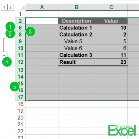
Select the whole area in which you suspect hidden rows. Alternatively select the whole worksheet in the top left corner.
>Now double-click on the border between two row numbers (number 5 in the screenshot above). Each row has now it’s minimum size to cover all it’s contents. There is one disadvantage, though: The row height of all selected rows will be reset. So, if you have already set the row heights manually, it will be gone.
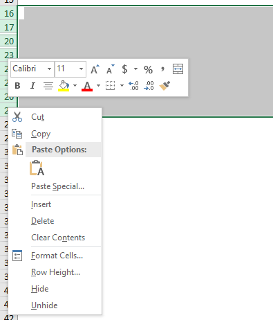
Instead of double-clicking according to the number two above you can right-click on the column or row header (that means the column letter above your hidden column or the row number on the left-hand side). Next, click on “Unhide”.

Method 2: Use Professor Excel Tools

hide, unhide, manager, rows, columns, add-in, excel

Hide or unhide rows and columns comfortably with Professor Excel Tools

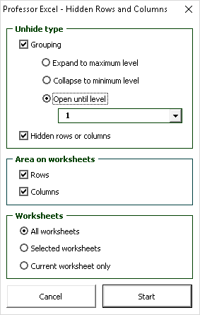
The Excel add-in Professor Excel Tools provide a function for unhiding all hidden rows and columns on all sheets with one click. Alternatively only unhide the rows or columns on the selected or current sheet.

To use the function, click on “Hidden Rows and Columns” in the “Professor Excel” ribbon. Now you’ll see a window as shown on the screenshot on the right-hand side.

This function is included in our Excel Add-In ‘Professor Excel Tools’

(No sign-up, download starts directly)

Henrik Schiffner is a freelance business consultant and software developer. He lives and works in Hamburg, Germany. Besides being an Excel enthusiast he loves photography and sports.

We use cookies on our website to give you the most relevant experience by remembering your preferences and repeat visits. By clicking “Accept”, you consent to the use of ALL the cookies.

Источник

You can hide and unhide rows in Excel by right-clicking, or reveal all hidden rows using the «Format» option in the «Home» tab.
Hiding rows in Excel is especially helpful when working in large documents or for concealing information you won’t need until later.
Visit Business Insider’s homepage for more stories.

Just as you can quickly hide and unhide columns, you can hide or reveal hidden rows in your Excel spreadsheet as well.

In addition to freezing rows, you may find it helpful to conceal rows you are no longer using without permanently deleting the data from your spreadsheet. To later reveal the hidden cells, you can right-click to unhide individual rows.

You can also navigate to the «Format» option to unhide all hidden rows. This feature is especially helpful if you’ve hidden multiple rows throughout a large spreadsheet.

Here’s how to do both.

Check out the products mentioned in this article:

Microsoft Office (From $139.99 at Best Buy)

MacBook Pro (From $1,299.99 at Best Buy)

Microsoft Surface Pro X (From $999 at Best Buy)

How to hide individual rows in Excel

1. Open Excel.

2. Select the row(s) you wish to hide. Select an entire row by clicking on its number on the left hand side of the spreadsheet. Select multiple rows by clicking on the row number, holding the «Shift» key on your Mac or PC keyboard, and selecting another.

3. Right-click anywhere in the selected row.

4. Click «Hide.»

How to unhide rows in Excel

Right-click to hide rows.

Marissa Perino/Business Insider

How to unhide individual rows in Excel

1. Highlight the row on either side of the row you wish to unhide.

2. Right-click anywhere within these selected rows.

3. Click «Unhide.»

How to unhide rows in Excel

Highlight adjacent cells to unhide a hidden row.

Marissa Perino/Business Insider

4. You can also manually click or drag to expand a hidden row. Hidden rows are indicated by a thicker border line. Move your cursor over this line until it turns into a double bar with arrows. Double click to reveal or click and drag to manually expand the hidden row or rows. (If you’ve hidden multiple rows, you may have to do this multiple times.)

1. To unhide all hidden rows in Excel, navigate to the «Home» tab.

2. Click «Format,» which is located towards the right hand side of the toolbar.

3. Navigate to the «Visibility» section. You’ll find options to hide and unhide both rows and columns.

4. Hover over «Hide & Unhide.»

5. Select «Unhide Rows» from the list. This will reveal all hidden rows, a feature especially helpful if you’ve hidden multiple rows throughout a large spreadsheet.

How to unhide rows in Excel

Unhide all rows.

Marissa Perino/Business Insider

Related coverage from How To Do Everything: Tech:

How to make a line graph in Microsoft Excel in 4 simple steps using data in your spreadsheet
How to add a column in Microsoft Excel in 2 different ways
How to hide and unhide columns in Excel to optimize your work in a spreadsheet
How to search for terms or values in an Excel spreadsheet, and use Find and Replace

Marissa Perino is a former editorial intern covering executive lifestyle. She previously worked at Cold Lips in London and Creative Nonfiction in Pittsburgh. She studied journalism and communications at the University of Pittsburgh, along with creative writing. Find her on Twitter: @mlperino.

Unhide all rows in Excel

Identifying hidden rows requires you to look very carefully at all the row numbers.

This is cumbersome⏳

So you definitely want to use one of several techniques to unhide all rows at once.

1. Select the rows where you think there are hidden rows in between.

Since you can’t select the specific hidden rows, you need to drag “over” them with your cursor while holding down the left mouse button.

2. Right-click any of the selected rows.

3. Click Unhide.

Right click selected rows and click Unhide

That’s it – now all the hidden rows in between the rows you selected are visible💡

Unhide rows with shortcut

Unhiding rows can be done even faster than this!

After selecting the rows in step 1 above, you can use a shortcut to unhide rows instead of doing step 2 and 3.

So, select the rows and press Ctrl + Shift + 9.

Easy, huh?

Unhide rows hidden by autofilter

Sometimes rows are hidden because of another method: the autofilter.

With the autofilter, you can easily control which rows are visible (and which are hidden).

To unhide rows hidden by the autofilter, you don’t need to jump through all the hoops.

Simply go to the Data tab, and click the Clear button.

Unhide individual or multiple rows

Sometimes, you don’t want to unhide all rows, but just a specific row, or several specific rows.

To unhide multiple rows, use the same method as before:

1. Select the cell above the hidden rows, hold down your left mouse button and drag over the hidden rows – selecting them and the row below the hidden rows.

2. Right-click any of the 2 visible selected rows.

3. Click Unhide.

And voila! The rows are visible👓

Unhide first row in Excel

Unhiding the first row can be particularly tricky – if you don’t know how.

Because, how can you select it if you can’t “drag over” it, like with other hidden rows?

Luckily, there’s another way to select that first hidden row.

1. To the left of the formula bar there’s a name box. Write “A1” in it.

Now, cell A1 is selected.

2. On the right side of the Home tab, click Format.

3. Hover the cursor over ‘Hide & Unhide’ and click ‘Unhide Rows’.

Now, the first row is visible again 👍

PRO TIP:

If you find the above method for unhiding the first row a bit too cumbersome, try this instead.

You can actually select the hidden first row by holding down the left mouse button and “dragging over” it.

You just need to start dragging from row 2 and then drag in an upwards motion that ends on row 0 (the grey triangle).

Select first hidden row by dragging over row 1

After that, just right-click row 2 and click Unhide.

Note: it’s not enough to just select row 2. You need to drag over row 1.

Unhide columns in Excel

Hidden columns can be almost as cumbersome to identify as rows.

I’ve sung the alphabet song to myself countless times to try and identify which letters (column names) were missing.

Here’s how to do it without singing🎶

1. Select the columns where you believe columns are hidden in between. You do that by “dragging over” them while holding down the left mouse button.

2. Right-click any of the visible selected columns.

3. Click Unhide.

Unhide all rows and columns

This is your one-stop solution for unhiding all the rows and columns in your spreadsheet.

You don’t have to look for anything or spend a second thinking if you “dragged over” all the rows that could have a hidden row in between.

Kasper Langmann, Microsoft Office Specialist

Here’s how to unhide all the hidden rows and all the hidden columns in one fell swoop.

1. Select all the cells in the spreadsheet by clicking the ‘Select All’ button.

Or you can use the Ctrl + A shortcut.

2. Right-click any of the selected rows and click Unhide.

This unhides all the hidden rows.

3. Right-click any of the selected columns and click Unhide.

This unhides all the columns.

And that’s how you unhide all rows and columns at once🔍

VIDEO: Unhide rows and columns

That’s it – Now what?

You just learned how to unhide all rows in Excel.

And a lot more, actually!

It wasn’t so scary after all, was it?😎

You’re unhiding rows because you want to work with the full data set, instead of just the visible part of it.

So, now that your hidden rows are visible, you should consider learning a few methods to work professionally with your data.

No matter your current skill level, I got you covered.

Click here and enroll in my free 30-minute online training.

I’ll send it directly to your inbox within 5 minutes.

Other resources

If you’ve made hidden rows visible but didn’t mean to, you can simply undo your actions with the Undo feature.

Or you can hide rows to make the data set the same as it was before.

Also, as I mentioned before, filters are a great way to work better with big data sets by hiding rows you don’t want to look at.

FAQ

Got any specific questions about unhiding rows?

Read below and you may find your answer😊

This might be because:

A) The rows are hidden by an autofilter. Go to the Data tab and click the Clear button next to the filter button.

B) The rows are not hidden but are very small. Drag over the small rows with your cursor. Right-click any of the rows and select ‘Row Height’. Type 15 and click ‘OK’.

Unhiding rows is the same on MAC and Windows. Select the hidden row by dragging over it with your cursor. Then right-click and select the Unhide option.

These steps are the same when unhiding columns in Excel for MAC, except you select columns and not rows.

Kasper Langmann2023-02-23T14:43:41+00:00

Page load link

Источник

How to unhide all rows in excel

About This Article

Is this article up to date?

Hide or show rows or columns

Hide columns

Unhide columns

Need more help?

See Also

Need more help?

Method 1: Unhide all rows or columns manually

Hide rows and columns

Unhide rows and columns

Method 2: Use Professor Excel Tools

Check out the products mentioned in this article:

Microsoft Office (From $139.99 at Best Buy)

MacBook Pro (From $1,299.99 at Best Buy)

Microsoft Surface Pro X (From $999 at Best Buy)

How to hide individual rows in Excel

How to unhide individual rows in Excel