
If you have a worksheet with data in columns that you need to rotate to rearrange it in rows, use the Transpose feature. With it, you can quickly switch data from columns to rows, or vice versa.
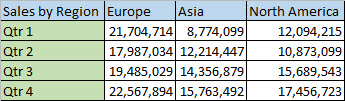
For example, if your data looks like this, with Sales Regions in the column headings and and Quarters along the left side:
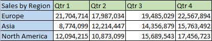
The Transpose feature will rearrange the table such that the Quarters are showing in the column headings and the Sales Regions can be seen on the left, like this:
Note: If your data is in an Excel table, the Transpose feature won’t be available. You can convert the table to a range first, or you can use the TRANSPOSE function to rotate the rows and columns.
Here’s how to do it:
-
Select the range of data you want to rearrange, including any row or column labels, and press Ctrl+C.
Note: Ensure that you copy the data to do this, since using the Cut command or Ctrl+X won’t work.
-
Choose a new location in the worksheet where you want to paste the transposed table, ensuring that there is plenty of room to paste your data. The new table that you paste there will entirely overwrite any data / formatting that’s already there.
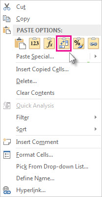
Right-click over the top-left cell of where you want to paste the transposed table, then choose Transpose
 .
.
-
After rotating the data successfully, you can delete the original table and the data in the new table will remain intact.
 .
.
Tips for transposing your data
-
If your data includes formulas, Excel automatically updates them to match the new placement. Verify these formulas use absolute references—if they don’t, you can switch between relative, absolute, and mixed references before you rotate the data.
-
If you want to rotate your data frequently to view it from different angles, consider creating a PivotTable so that you can quickly pivot your data by dragging fields from the Rows area to the Columns area (or vice versa) in the PivotTable Field List.
You can paste data as transposed data within your workbook. Transpose reorients the content of copied cells when pasting. Data in rows is pasted into columns and vice versa.
Here’s how you can transpose cell content:
-
Copy the cell range.
-
Select the empty cells where you want to paste the transposed data.
-
On the Home tab, click the Paste icon, and select Paste Transpose.
Excel for Microsoft 365 Excel for Microsoft 365 for Mac Excel for the web Excel 2021 Excel 2021 for Mac Excel 2019 Excel 2019 for Mac Excel 2016 Excel 2016 for Mac Excel 2013 Excel 2010 Excel 2007 Excel for Mac 2011 Excel Starter 2010 More…Less
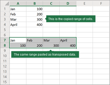
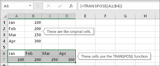
Sometimes you need to switch or rotate cells. You can do this by copying, pasting, and using the Transpose option. But doing that creates duplicated data. If you don’t want that, you can type a formula instead using the TRANSPOSE function. For example, in the following picture the formula =TRANSPOSE(A1:B4) takes the cells A1 through B4 and arranges them horizontally.
Note: If you have a current version of Microsoft 365 , then you can input the formula in the top-left-cell of the output range, then press ENTER to confirm the formula as a dynamic array formula. Otherwise, the formula must be entered as a legacy array formula by first selecting the output range, input the formula in the top-left-cell of the output range, then press Ctrl+Shift+Enter to confirm it. Excel inserts curly brackets at the beginning and end of the formula for you. For more information on array formulas, see Guidelines and examples of array formulas.
Step 1: Select blank cells
First select some blank cells. But make sure to select the same number of cells as the original set of cells, but in the other direction. For example, there are 8 cells here that are arranged vertically:

So, we need to select eight horizontal cells, like this:

This is where the new, transposed cells will end up.
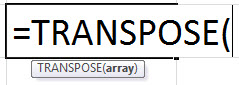
Step 2: Type =TRANSPOSE(
With those blank cells still selected, type: =TRANSPOSE(
Excel will look similar to this:
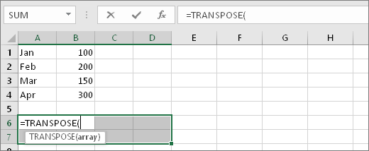
Notice that the eight cells are still selected even though we have started typing a formula.
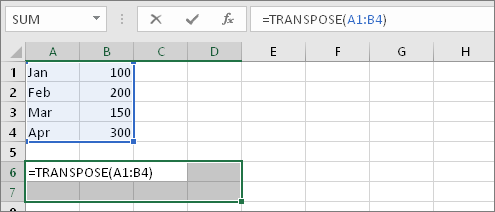
Step 3: Type the range of the original cells.
Now type the range of the cells you want to transpose. In this example, we want to transpose cells from A1 to B4. So the formula for this example would be: =TRANSPOSE(A1:B4) — but don’t press ENTER yet! Just stop typing, and go to the next step.
Excel will look similar to this:
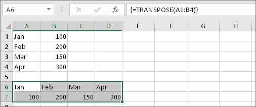
Step 4: Finally, press CTRL+SHIFT+ENTER
Now press CTRL+SHIFT+ENTER. Why? Because the TRANSPOSE function is only used in array formulas, and that’s how you finish an array formula. An array formula, in short, is a formula that gets applied to more than one cell. Because you selected more than one cell in step 1 (you did, didn’t you?), the formula will get applied to more than one cell. Here’s the result after pressing CTRL+SHIFT+ENTER:
Tips
-
You don’t have to type the range by hand. After typing =TRANSPOSE( you can use your mouse to select the range. Just click and drag from the beginning of the range to the end. But remember: press CTRL+SHIFT+ENTER when you are done, not ENTER by itself.
-
Need text and cell formatting to be transposed as well? Try copying, pasting, and using the Transpose option. But keep in mind that this creates duplicates. So if your original cells change, the copies will not get updated.
-
There’s more to learn about array formulas. Create an array formula or, you can read about detailed guidelines and examples of them here.
Technical details
The TRANSPOSE function returns a vertical range of cells as a horizontal range, or vice versa. The TRANSPOSE function must be entered as an array formula in a range that has the same number of rows and columns, respectively, as the source range has columns and rows. Use TRANSPOSE to shift the vertical and horizontal orientation of an array or range on a worksheet.
Syntax
TRANSPOSE(array)
The TRANSPOSE function syntax has the following argument:
-
array Required. An array or range of cells on a worksheet that you want to transpose. The transpose of an array is created by using the first row of the array as the first column of the new array, the second row of the array as the second column of the new array, and so on. If you’re not sure of how to enter an array formula, see Create an array formula.
See Also
Transpose (rotate) data from rows to columns or vice versa
Create an array formula
Rotate or align cell data
Guidelines and examples of array formulas
Need more help?
The concept of «transport» almost does not occur in the work of PC users, but those ones who work with arrays, whether matrices in higher mathematics or the tables in Excel, have to face with this phenomenon necessary.
Transposing a table in Excel is the replacement of columns by rows and vice versa. In other words, it is a turn in two planes: horizontal and vertical ones. There are three ways to transport tables.
The method 1: the special insert
It`s the simplest and universal way. Let’s consider at once on an example. We have the table with the price of a certain product per a piece and with certain amount of products. The table cap is located horizontally, and the data is arranged vertically, respectively. The cost is calculated by the formula: price * quantity. For the sake of the clarity, the table header is highlighted in green color.
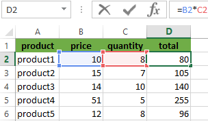
We need to arrange the table`s data horizontally relative to the vertical arrangement of its header.
To transpose the table, we will use the SPECIAL INSERT command. We proceed in these steps:
- We select the entire table and copy it (CTRL + C).
- We put the cursor anywhere in the Excel worksheet and right-click the menu.
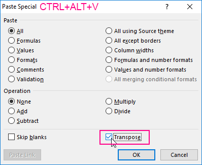
- We click on the command Paste Special (CTRL+ALT+V).
- In the window that appears we put the tick near the TRANSPOSE. The rest we left as is and click OK.
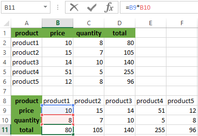
As a result we obtained the same table, but with different arrangement of the rows and the columns. Moreover, we note that cells with the same content are highlighted in green. The value formula was also copied and counted the product of price and quantity, but already with taking into account other cells. Now the table header is located vertically (what is clearly visible due to the green color of the header), and the data are respectively located horizontally.
Similarly, only values can be transposed, without the names of rows and the columns. To do this, you need to select only the array with the values and to do the same with the «Paste Special» command.
The method 2: the TRANSPOSE function in Excel
With the advent of the SPECIAL INSERT, the transposing of the table with using the TRANSPOSE command is almost not used because of the complexity and longer time for the operation. But the TRANSPOSE function is still present in Excel, so we will learn how to use it.
We operate on the stages again:
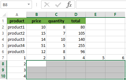
- We select correctly to the range for transposing. In this example of the source table there are 4 columns and 6 rows. Accordingly, we must select the range of the cells in what there will be 6 columns and 4 rows. As it shown on the picture:
- We fill immediately to the active cell so that you do not remove the selected area and enter the following formula: =TRANSPOSE.
- To press CTRL + SHIFT + ENTER. Attention! The function TRANSPOSE() works only in an array. Therefore, after entering it, you must necessarily press the combination of the hotkeys CTRL + SHIFT + ENTER to execute the function in the array, and not just ENTER.

Note that the formula was not copied. When you click on the each cell, you will see that this table has been transposed. In addition, all the original formatting has been lost and you have to align and backlight it again. Also worth paying attention to the fact that the transposed table is tied to the original one. The modified values of the source table are automatically updated in the transposed one.
The method 3: the PivotTable
Those who work closely with Excel know that the PivotTable is multifunctional. And possibility of transpose – is one of its functions. Although it will be look a little bit different than in the previous examples.
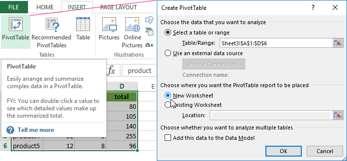
- We will create to the PivotTable. To do this, you need to select the original table and open the INSERT — PivotTable item.
- The place where the summary table will be created, we select the new sheet.
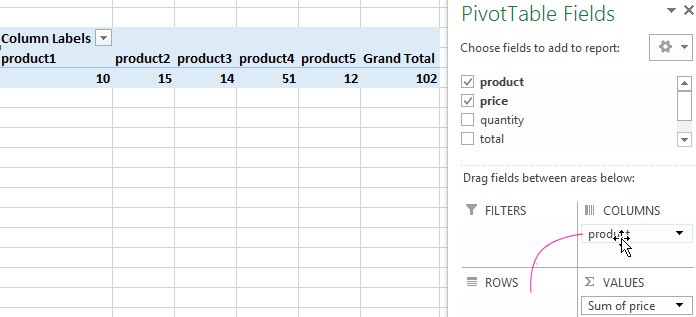
- In the resulting layout of the summary tables, we can select the necessary items and move them to the required fields. We will transfer «product» in the NAMES of COLUMNS, and «the price per piece» in VALUES.
- We obtained the PivotTable for the required field, and the team automatically calculated the grand total.
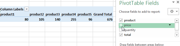
- You can remove the tick from the PRICE and tick off it next to the TOTAL PRICE. And then we get the PivotTable for the value of goods, as well as the grand total again.
Download example transpose data in Excel.
This is a rather peculiar method of partial transposition, which allows you to replace the columns in the rows (on the contrary — it does not work) and additionally learn to the total amount of the given field.
What Does Transpose Function Do in Excel?
The TRANSPOSE function in excel helps rotate (switch) the values from rows to columns and vice versa. Being a part of the Excel lookup and reference functions, its purpose is to organize the data in the desired format. To execute the formula, the exact size of the range to be transposed is selected and the CSE key (“Control+Shift+Enter”) is pressed.
The Syntax of the TRANSPOSE Function
The syntax of the function is stated as follows:
The function accepts the following mandatory argument:
Array: This is the range of cells that are to be transposed.
Table of contents
- What Does Transpose Function Do in Excel?
- The Syntax of the TRANSPOSE Function
- How to use the TRANSPOSE Function in Excel?
- Example #1
- Example #2
- Example #3
- Example #4
- Example #5
- Example #6
- The Characteristics of the TRANSPOSE Function
- Frequently Asked Questions
- Recommended Articles
How to use the TRANSPOSE Function in Excel?
You can download this TRANSPOSE Function Excel Template here – TRANSPOSE Function Excel Template
Example #1
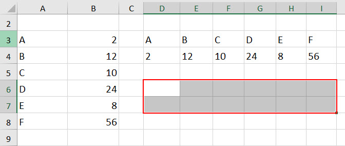
The following table consists of data points in the cells A3:B8. The cells D3:I4 are transposed by copy-pasting the original data.
We want to transpose the given range (A3:B8) with the help of the TRANSPOSE excel function.

The steps to transpose the range A3:B8 are listed as follows:
- Select the range D6:I7 where the transposed values should appear.

- Enter the following TRANSPOSE excel formula in the selected region (shown in the succeeding image).
“=TRANSPOSE (A3:B8)”

- Press “Ctrl+Shift+Enter” (“Command+Shift+Enter” in Mac).
The transposed output in D6:I7 is shown in the following image. As soon as the CSE key is pressed, the TRANSPOSE formula appears within the curly braces.
“{=TRANSPOSE (A3:B8)}”
The curly braces {} indicate that an array formula has been entered.


The Transposed Output
The range D3:I4 is transposed by the copy-pasteTranspose is the process of swapping columns with rows in Excel. Because this function is linked to cells, any changes done are reflected in transposed data.read more method, while D6:I7 is transposed by the TRANSPOSE function. The two ranges are shown in the succeeding image.
If a value of the original data is changed, the output transposed by the TRANSPOSE function updates automatically. However, the output transposed by the copy-paste method remains the same.
Note: The copy-paste option creates duplicates.

Example #2
Let us use the TRANSPOSE function in combination with the IF function.
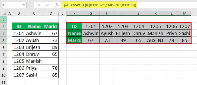
The following table shows the average marks of seven students in a school. For the students who did not appear in the examination, the “marks” field has been left blank.
In addition to transposing the given data, we want to enter “absent” in the empty cell.

Enter the following formula to use the TRANSPOSE and the IF functionsIF function in Excel evaluates whether a given condition is met and returns a value depending on whether the result is “true” or “false”. It is a conditional function of Excel, which returns the result based on the fulfillment or non-fulfillment of the given criteria.
read more together.
“=TRANSPOSE(IF(B3:D10=””,”ABSENT”,B3:D10))”
The two functions check whether a cell is blank or not. If a cell in the range B3:D10 is empty, the word “ABSENT” is returned. Otherwise, the formula is supplied a value to transpose.
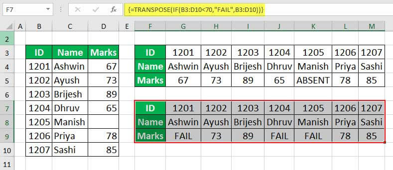
Example #3
Working on the data of example #2, let us modify the criteria.
A student is considered to have failed if either of the following is true:
- The average marks are less than 70.
- He/she has not appeared in the examination.
To meet the preceding criteria, enter the following formula.
“=TRANSPOSE(IF(B3:D10<70,”FAIL”,B3:D10)”
The output is shown in the following image.
Example #4
There is a list of IDs in the range B4:B7. We want to prefix the acronym ID with the help of the TRANSPOSE function.
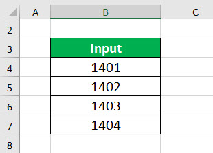
Enter the following formula.
“=TRANSPOSE(“ID”&B4:B7)”

The range is transposed and the prefix is added to every cell, as shown in the following image. Likewise, a suffix can also be added by using the TRANSPOSE formula.

Example #5
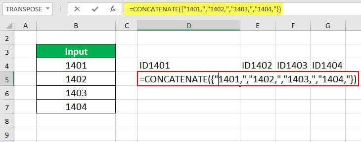
The TRANSPOSE and CONCATENATE functionsThe CONCATENATE function in Excel helps the user concatenate or join two or more cell values which may be in the form of characters, strings or numbers.read more are used together to combine the words of different rows in a single cell. The steps are listed as follows:
Step 1: Type the formula “=CONCATENATE(TRANSPOSE(B4:B7&”,”))”.
![]()
Step 2: Press the F9 key. The CONCATENATE function with IDs appears (shown in the following image).
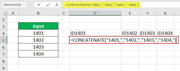
Step 3: Remove the curly braces {} from the formula.
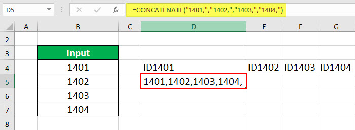
Step 4: Press the “Enter” key. The numbers of the range B4:B7 are combined in the single cell D5. The output is shown in the following image.
Example #6
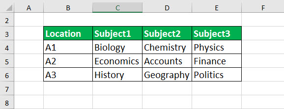
The following table shows the books on different subjects in a library. Every book is placed on a shelf denoted by the location.
We want to retrieve the location of the books (second subsequent image) using the data in the range B4:E6.
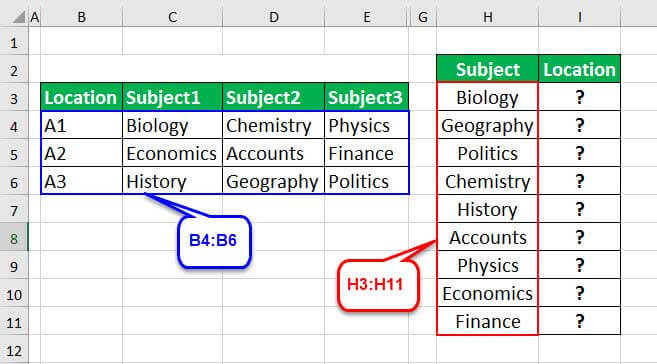
We use the following formula.
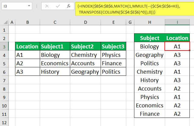
“=INDEX($B$4:$B$6,MATCH(1,MMULT(–($C$4:$E$6=<Subject>),TRANSPOSE(COLUMN($C$4:$E$6)^0)),0))”
The Explanation of the Preceding Formula
In the following pointers, a part of the formula is displayed, followed by an explanation.
- “–($C$4:$E$6=<Subject>)”
The field <subject> corresponds to the cell H3. So, the formula becomes “–($C$4:$E$6=H3).”
This creates an array of “1” and “0” which indicates the presence or absence of a value. For instance, the book “biology” shown in H3 is represented as {1,0,0;0,0,0;0,0,0}.
- “TRANSPOSE(COLUMN($C$4:$E$6)^0))”
This creates an array of three rows in a column. The “0” of the formula ensures that the numbers are converted to “1.” So, the output of this function is {1,1,1}.
- “MMULT(–($C$4:$E$6=<Subject>),TRANSPOSE(COLUMN($C$4:$E$6)^0))”
The MMULTMMULT is an in-built Math & Trigonometry function in Excel that performs matrix multiplication of 2 arrays where the columns of Array 1 are equivalent to the rows for Array 2. read more multiplies the output of A and B. So, “MMULT({1,0,0;0,0,0;0,0,0}, {1,1,1})” gives the output {1;0;0}.
- “MATCH(1,MMULT(<..>),0)”
This matches the output of column C with 1. “MATCH(1,{1;0;0},0)” returns the position 1.
- “INDEX($B$4:$B$6,MATCH(<…>,0))”
This identifies the cell value for which the position is specified by the MATCH functionThe MATCH function looks for a specific value and returns its relative position in a given range of cells. The output is the first position found for the given value. Being a lookup and reference function, it works for both an exact and approximate match. For example, if the range A11:A15 consists of the numbers 2, 9, 8, 14, 32, the formula “MATCH(8,A11:A15,0)” returns 3. This is because the number 8 is at the third position.
read more. So, “INDEX($B$4:$B$6,1)” returns A1.
The Output for the Book “Geography”
Similar to the book “Biology,” the output for the book “Geography” is listed as follows:
- “–($C$4:$E$6=D6)” returns {0,0,0;0,0,0;0,1,0}.
- “TRANSPOSE(COLUMN($C$4:$E$6)^0))” returns {1,1,1}.
- “MMULT({0,0,0;0,0,0;0,1,0},{1,1,1})” returns {0;0;1}.
- “MATCH(1,{0;0;1},0)” returns 3.
- “INDEX($B$4:$B$6,3)” returns A3.
The Characteristics of the TRANSPOSE Function
The features of the function are listed as follows:
- It links the data to the source.
- It returns the #VALUE error#VALUE! Error in Excel represents that the reference cell the user has either entered an incorrect formula or used a wrong data type (mostly numerical data). Sometimes, it is difficult to identify the kind of mistake behind this error.read more if the number of rows and columns selected are not equal to the columns and rows of the source data.
- Once entered, any individual cell which is a part of this function cannot be changed.
Frequently Asked Questions
1. Define the Excel TRANSPOSE function.
The TRANSPOSE function in excel flips the orientation of a range from horizontal to vertical and vice versa. The syntax is stated as follows:
“=TRANSPOSE(array)”
With the TRANSPOSE function, the first row of the array (data source) becomes the first column of the new array (output). Likewise, the second row of the old array becomes the second column of the new array and so on. A change in the data source and the output transposed by the function automatically updates.
Note: The TRANSPOSE function does not copy cell formatting. It only copies the cell values.
2. How to transpose the rows and columns in Excel?
3. How is the TRANSPOSE excel function used?
The steps to use the function are listed as follows:
– Count the number of rows and columns of the original data source.
– Select an empty range with the same number of rows as the columns of the old array and vice versa.
– Type the TRANSPOSE formula and press “Ctrl+Shift+Enter.”
The transposed output appears in the selected range.
- The TRANSPOSE function helps rotate the values from rows to columns and vice versa.
- The TRANSPOSE function accepts one mandatory argument–“array,” representing the range to be transposed.
- Prior to executing the TRANSPOSE formula, the exact size of the range to be transposed is selected.
- Being an array function, the TRANSPOSE formula is entered by pressing “Ctrl+Shift+Enter.”
- A range can be transposed by the TRANSPOSE function, the INDIRECT and ADDRESS functions, the “paste special” option, and so on.
- The TRANSPOSE function is used in combination with IF, CONCATENATE, INDEX, MATCH, etc., to get the desired output.
Recommended Articles
This has been a guide to the TRANSPOSE function in Excel. Here we discuss how to use TRANSPOSE formula in Excel with example and downloadable templates. You may also look at these useful functions in Excel –
- Copy Paste in Excel VBAIn VBA, we use the copy method with range property to copy a value from one cell to another. To paste the value, we use the worksheet function paste exceptional or paste method.read more
- VBA IsEmptyIsEmpty is a worksheet function that determines whether or not a certain cell reference or a range of cells is empty. We use the Application Worksheet method in VBA to use it.read more
- Paste Special in VBAPaste Special in VBA allows us to paste data as is or only formulas or values, and we can paste special using the range property method, as shown below: Paste special() providing the type we want in the brackets.read more
- SWITCH Function in ExcelSwitch function in excel is a comparison and referencing function which compares and matches a referred cell to a group of cells and returns the result based on the first match found. The method to use this function is =SWITCH( target cell, value 1, result 1….).read more
Watch Video – How to Transpose Data in Excel
If you have a dataset and you want to transpose it in Excel (which means converting rows into columns and columns into rows), doing it manually is a complete NO!
Transpose Data using Paste Special
Paste Special can do a lot of amazing things, and one such thing is to transpose data in Excel.
Suppose you have a dataset as shown below:
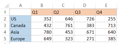
This data has the regions in a column and quarters in a row.
Now for some reason, if you need to transpose this data, here is how you can do this using paste special:
This would instantly copy and paste the data but in such a way that it has been transposed. Below is a demo showing the entire process.
The steps shown above copies the value, the formula (if any), as well as the format. If you only want to copy the value, select ‘value’ in the paste special dialog box.
Note that the copied data is static, and if you make any changes in the original data set, those changes would not be reflected in the transposed data.
If you want these transposed cells to be linked to the original cells, you can combine the power of Find & Replace with Paste Special.
Transpose Data using Paste Special and Find & Replace
Using Paste Special alone gives you static data. This means that if your original data changes and you want the transposed data to be updated as well, then you need to use Paste Special again to transpose it.
Here is a cool trick you can use to transpose the data and still have it linked with the original cells.
Suppose you have a dataset as shown below:
Here are the steps to transpose the data but keep the links intact:
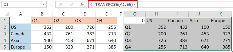
- Select the data set (A1:E5).
- Copy it (Control + C, or right-click and select copy).

- Now you can paste the transposed data in a new location. In this example, I want to copy in G1:K5, so right-click on cell G1 and select paste special.

- In the Paste Special dialog box, click on the Paste Link button. This will give you the same data set, but here the cells are linked to the original data set (for example G1 is linked to A1, and G2 is linked to A2, and so on).
- With this new copied data selected, Press Control + H (or go to Home –> Editing –> Find & Select –> Replace). This will open the Find & Replace dialog box.

- In the Find & Replace dialog box, use the following:
- In Find what: =
- In Replace with: !@# (note that I am using !@# as it’s a unique combination of characters that is unlikely to be a part of your data. You can use any such unique set of characters).

- Click on Replace All. This will replace the equal to from the formula and you will have !@# followed by the cell reference in each cell.
- Right-click and copy the data set (or use Control + C).
- Select a new location, right-click and select paste special. In this example, I am pasting it in cell G7. You can paste it anywhere you want.
- In the Paste Special dialog box, select Transpose and click OK.
- Copy paste this newly created transposed data to the one from which it is created.

- Now open the Find and Replace dialog box again and replace !@# with =.


This will give you a linked data that has been transposed. If you make any changes in the original data set, the transposed data would automatically update.
Note: Since our original data has A1 as empty, you would need to manually delete the 0 in G1. The 0 appears when we paste links, as a link to an empty cell would still return a 0. Also, you’d need to format the new dataset (you can simply copy paste the format only from the original dataset).
Transpose Data using Excel TRANSPOSE Function
Excel TRANSPOSE function – as the name suggests – can be used to transpose data in Excel.
Suppose you have a dataset as shown below:
Here are the steps to transpose it:
- Select the cells where you want to transpose the dataset. Note that you need to select the exact number of cells as the original data. So for example, if you have 2 rows and 3 columns, you need to select 3 rows and 2 columns of cells where you want the transposed data. In this case, since there are 5 rows and 5 columns, you need to select 5 rows and 5 columns.

- Enter =TRANSPOSE(A1:E5) in the active cell (which should be the top left cell of the selection and press Control Shift Enter.

This would transpose the dataset.
Here are a few things you need to know about the TRANSPOSE function:
- It is an array function, so you need to use Control-Shift-Enter and not just Enter.
- You can not delete a part of the result. You need to delete the entire array of values that the TRANSPOSE function returns.
- Transpose function only copies the values, not the formatting.
Transpose Data Using Power Query
Power Query is a powerful tool that enables you to quickly transpose data in Excel.
Power Query is a part of Excel 2016 (Get & Transform in the Data tab) but if you’re using Excel 2013 or 2010, then you need to install it as an add-in.
Suppose you have the data set as shown below:
Here are the steps to transpose this data using Power Query:
In Excel 2016
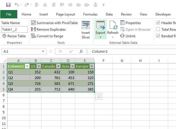
Note that since the top left cell of our data set was empty, it gets a generic name Column1 (as shown below). You can delete this cell from the transposed data.
In Excel 2013/2010
In Excel 2013/10, you need to install Power Query as an add-in.
Click here to download the plugin and get installation instructions.
Once you have installed Power Query, go to Power Query –> Excel Data –> From Table.
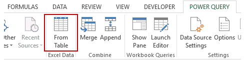
This will open the create table dialog box. Now follow the same steps as shown for Excel 2016.
You May Also Like the Following Excel Tutorials:
- Multiply in Excel using Paste Special.
- CONCATENATE Excel Range (with and without separator).
- Clean Data in Excel Spreadsheets.
- Compare Columns in Excel
- Excel Text to Columns
- Excel TRIM Function
- Merge Tables in Excel