
Often, users need to raise a number to a power. How to do it correctly with the help of «Excel»?
In this article, we will try to understand popular user questions and give instructions on how to use the system correctly. MS Office Excel allows you to perform a number of mathematical functions: from the simplest to the most complex. This universal software is designed for all occasions.
How to raise to the power of in excel?
Before searching for the required function, pay attention to the mathematical laws:
- «1» will remain «1» to any degree.
- «0» will remain «0» to any degree.
- Any number raised to zero degree equals one.
- Any value of «A» in the power of «1» will be equal to «A».
Examples in Excel:
Variant 1. Use the character «^»
The standard and easiest option is to use the «^» icon, which is obtained by pressing Shift + 6 with the English keyboard layout.
IMPORTANT!
- In order for the number to be exponentiation to the required degree, it is necessary to put the «=» sign in the cell before specifying the number you want to build.
- The degree is indicated after the sign «^».
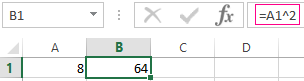
We built 8 into a «square» (that is, to the second degree) and got the result of the calculation in cell «A2».
Variant 2. Using the function
In Microsoft Office Excel there is a convenient function «POWER», which you can activate for simple and complex mathematical calculations
The function looks like this:
=POWER(Number,Degree)
ATTENTION!
- The numbers for this formula are indicated without spaces or other signs.
- The first digit is the value «number». This is the basis (that is, the figure that we are building). Microsoft Office Excel allows the introduction of any real number.
- The second figure is the value of «degree». This is an indicator in which we build the first figure.
- The values of both parameters can be less than zero ( with a «-» sign).
Formula for the exponentiation in Excel
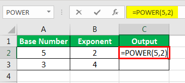
Examples of using the =POWER() function.
Using the function wizard:
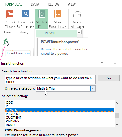
- Start the function wizard by using the hotkey combination SHIFT + F3 or click on the button at the beginning of the formula line «fx» (insert function). From the «Or select a category:» drop-down list, select «Math & Trig», and in the bottom field «Select a function:», specify the function «POWER» we need and click OK. Or select: «FORMULAS»-«Function Library»-«Math & Trig»-«POWER».
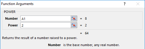
- In the dialog that appears, fill in the fields with arguments. For example, we need to exponentiate «2» to the degree of «3». Then in the first field enter «2», and in the second — «3».
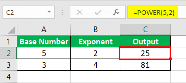
- Press the «OK» button and get in the cell into which the formula was entered, the value we need. For this situation, it is «2» in the «cube», i.e. 2 * 2 * 2 = 8. The program has calculated everything correctly and has given you the result.
If you think that extra clicks are a dubious pleasure, we offer one simpler variant.
Entering the function manually:
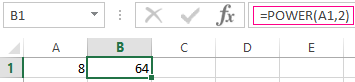
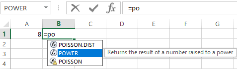
- In the formula line we put the sign «=» and begin to enter the name of the function. Usually it is enough to write «=po…» — and the system itself will guess to offer you a useful option.
- As soon as you saw such a hint, just press the «Tab» key. Or you can continue to write, manually enter each letter. Then in parentheses, specify the required parameters: two numbers separated by a semicolon.
- After that, click on «Enter» — and in the cell the calculated value 8 appears.
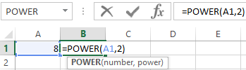
The sequence of actions is simple, and the user gets the result quickly enough. In arguments, instead of numbers, you can specify cell references.
Square root power in Excel
To extract the root using Microsoft Excel formulas, we use a slightly different, but very convenient, way of calling functions:
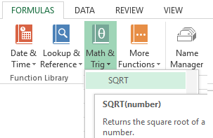
- Go to the «FORMULAS» tab. In the «Function Library» section of the toolbar, click on the «Math & Trig» tool. And from the drop-down list, select the «SQRT» option.
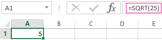
- Enter the function argument at the system request. In our case, it was necessary to find the root from «25», so we enter it into the line. After entering the number, just click on the «OK» button. In the cell, the figure obtained as a result of the mathematical calculation of the root will be reflected.
ATTENTION! If we need to know the root of the degree in Excel then we do not use the function =SQRT(). Let us recall the theory from mathematics:
«A root of the n-th degree of a is a number b whose n-th degree is equal to a«, that is:
n√a = b; bn = a
«A root of n-th degree from the number a will be equal to raising to the degree of the same number a by 1/n«, that is:
n√a = a1/n
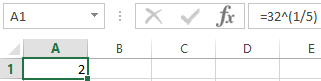
From this it follows that to calculate the mathematical formula of the root in the n-th degree for example:
5√32 = 2
In Excel, you should write through this formula: = 32 ^ (1/5), that is: = a ^ (1 / n) — where a is a number; N-degree:
Or through this function: =POWER(32,1/5)
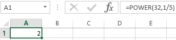
In the arguments of a formula and a function, you can specify cell references instead of the numbers.
How to write a number to the degree in Excel?
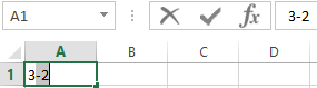
It is often important for you that the number in the degree is correctly displayed when printing and looks beautiful in the table. How to write a number to the degree in Excel? Here you need to use the Format Cells tab. In our example, we recorded «3» in the cell «A1», which should be presented to the -2 degree.
The sequence of actions is as follows:
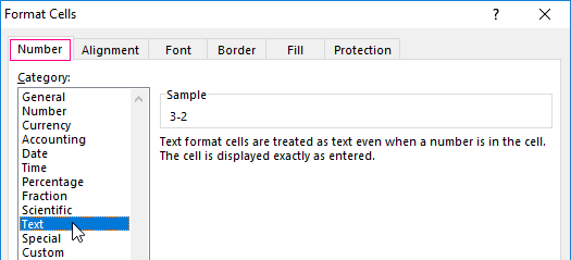
- Right click on the cell with the number and select the tab «Format Cells» from the pop-up menu. If it does not work out — find the «Format Cells» tab in the top panel or press CTRL + 1.
- In the menu that appears, select the «Number» tab and set the format for the «Text» cell. Click OK.
- In cell A1 enter «-2» next to «3» and select it.
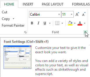
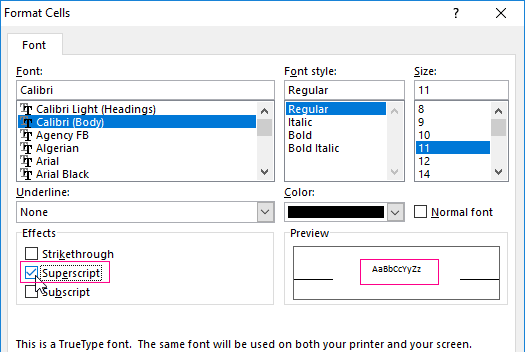
- Again, we call the format of cells (for example, by pressing CTRL + 1 hot keys) and now the «Font» tab is only available for us, where we tick the «Superscript» option. And click OK.
- The result should display the following meaning:
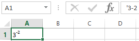
Using Excel’s features is easy and convenient. With them you save time on the implementation of mathematical calculations and the search for the necessary formulas.
Содержание
- How to raise a number to a power in Excel using the formula and operator
- How to raise to the power of in excel?
- Variant 1. Use the character «^»
- Variant 2. Using the function
- Formula for the exponentiation in Excel
- Square root power in Excel
- How to write a number to the degree in Excel?
- How to Insert or Show Power View in Excel?
- Steps to Insert Or Showing Power View
- Exponents in Excel
- Exponents in Excel Formula
- How to Use Exponents in Excel Formula?
- Method #1 – Using the Power Function
- Method #2 – Using Base Power
- Method #3 – Using the EXP Function
- Method #4 – Using theText-Based Exponents
- Things to Remember
- Recommended Articles
How to raise a number to a power in Excel using the formula and operator
Often, users need to raise a number to a power. How to do it correctly with the help of «Excel»?
In this article, we will try to understand popular user questions and give instructions on how to use the system correctly. MS Office Excel allows you to perform a number of mathematical functions: from the simplest to the most complex. This universal software is designed for all occasions.
How to raise to the power of in excel?
Before searching for the required function, pay attention to the mathematical laws:
- «1» will remain «1» to any degree.
- «0» will remain «0» to any degree.
- Any number raised to zero degree equals one.
- Any value of «A» in the power of «1» will be equal to «A».
Examples in Excel:
Variant 1. Use the character «^»
The standard and easiest option is to use the «^» icon, which is obtained by pressing Shift + 6 with the English keyboard layout.
- In order for the number to be exponentiation to the required degree, it is necessary to put the «=» sign in the cell before specifying the number you want to build.
- The degree is indicated after the sign «^».
We built 8 into a «square» (that is, to the second degree) and got the result of the calculation in cell «A2».
Variant 2. Using the function
In Microsoft Office Excel there is a convenient function «POWER», which you can activate for simple and complex mathematical calculations
The function looks like this:
- The numbers for this formula are indicated without spaces or other signs.
- The first digit is the value «number». This is the basis (that is, the figure that we are building). Microsoft Office Excel allows the introduction of any real number.
- The second figure is the value of «degree». This is an indicator in which we build the first figure.
- The values of both parameters can be less than zero ( with a «-» sign).
Formula for the exponentiation in Excel
Examples of using the =POWER() function.
Using the function wizard:
- Start the function wizard by using the hotkey combination SHIFT + F3 or click on the button at the beginning of the formula line «fx» (insert function). From the «Or select a category:» drop-down list, select «Math & Trig», and in the bottom field «Select a function:», specify the function «POWER» we need and click OK. Or select: «FORMULAS»-«Function Library»-«Math & Trig»-«POWER».

- In the dialog that appears, fill in the fields with arguments. For example, we need to exponentiate «2» to the degree of «3». Then in the first field enter «2», and in the second — «3».
- Press the «OK» button and get in the cell into which the formula was entered, the value we need. For this situation, it is «2» in the «cube», i.e. 2 * 2 * 2 = 8. The program has calculated everything correctly and has given you the result.
If you think that extra clicks are a dubious pleasure, we offer one simpler variant.
Entering the function manually:
- In the formula line we put the sign «=» and begin to enter the name of the function. Usually it is enough to write «=po…» — and the system itself will guess to offer you a useful option.
- As soon as you saw such a hint, just press the «Tab» key. Or you can continue to write, manually enter each letter. Then in parentheses, specify the required parameters: two numbers separated by a semicolon.
- After that, click on «Enter» — and in the cell the calculated value 8 appears.
The sequence of actions is simple, and the user gets the result quickly enough. In arguments, instead of numbers, you can specify cell references.
Square root power in Excel
To extract the root using Microsoft Excel formulas, we use a slightly different, but very convenient, way of calling functions:
- Go to the «FORMULAS» tab. In the «Function Library» section of the toolbar, click on the «Math & Trig» tool. And from the drop-down list, select the «SQRT» option.
- Enter the function argument at the system request. In our case, it was necessary to find the root from «25», so we enter it into the line. After entering the number, just click on the «OK» button. In the cell, the figure obtained as a result of the mathematical calculation of the root will be reflected.
ATTENTION! If we need to know the root of the degree in Excel then we do not use the function =SQRT(). Let us recall the theory from mathematics:
«A root of the n -th degree of a is a number b whose n -th degree is equal to a «, that is:
n √a = b; b n = a
«A root of n -th degree from the number a will be equal to raising to the degree of the same number a by 1/ n «, that is:
n √a = a 1/n
From this it follows that to calculate the mathematical formula of the root in the n -th degree for example:
5 √32 = 2
In Excel, you should write through this formula: = 32 ^ (1/5), that is: = a ^ (1 / n) — where a is a number; N-degree:
Or through this function: =POWER(32,1/5)
In the arguments of a formula and a function, you can specify cell references instead of the numbers.
How to write a number to the degree in Excel?
It is often important for you that the number in the degree is correctly displayed when printing and looks beautiful in the table. How to write a number to the degree in Excel? Here you need to use the Format Cells tab. In our example, we recorded «3» in the cell «A1», which should be presented to the -2 degree.
The sequence of actions is as follows:
- Right click on the cell with the number and select the tab «Format Cells» from the pop-up menu. If it does not work out — find the «Format Cells» tab in the top panel or press CTRL + 1.
- In the menu that appears, select the «Number» tab and set the format for the «Text» cell. Click OK.
- In cell A1 enter «-2» next to «3» and select it.
- Again, we call the format of cells (for example, by pressing CTRL + 1 hot keys) and now the «Font» tab is only available for us, where we tick the «Superscript» option. And click OK.
- The result should display the following meaning:
Using Excel’s features is easy and convenient. With them you save time on the implementation of mathematical calculations and the search for the necessary formulas.
Источник
How to Insert or Show Power View in Excel?
Power View is one of the features of excel, which enables us to visualize, explore and present large data sets and encourage ad-hoc reporting. The larger data sets can be easily visualized and analyzed in excel using the Power View and this data visualization is dynamic which helps to present the data within a single power view ad-hoc report. Ad-hoc, a Latin word used for “to this”, is also understood to be “as needed” or “as required”. When the reports are created on request it is termed ad-hoc reporting.
Steps to Insert Or Showing Power View
Let’s see how we can insert the power view in our excel document.
Step 1: Adding Power View. By default, Power View is not added to the excel ribbon (tools tab). In order to add it, we need to customize our ribbon. For this, we can use any tab(here, in this example we are using data-tab) Right-Click > Customize the Ribbon.

Once we click on the Customize the Ribbon option, excel will open a popup window where we are required to set the Power View option.

As we can see, we do not have a Power View option in our Data menu.
Step 2: Creating A New Group. In this step, we will create a new group for our Power View option. For this Select Data > New Group. This will create a New Group in the Data menu.

Step 3: Rename Group. In this step, we will rename our group. For this Select New Group > Rename. This will open a popup window to rename the group that we have created. (Here, we have renamed the group to Power View).

Once we click OK, our group will be renamed to Power View.
Step 4: Adding Command. In this step, we are required to add command to our Power View group. For this Select Power View > Choose commands from > All Commands.

After choosing All Commands from the drop-down list, we need to scroll-down and choose the Power View option.

After selecting Power View option from the All Commands tab, we need to click on Add button this will include Power View in our custom Power View group, and then click on the OK button.

Step 5: Output. Once we click on OK button, excel will add Power View to our selected tools tab. (Here, it is in Data).
Источник
Exponents in Excel

Exponents in Excel Formula
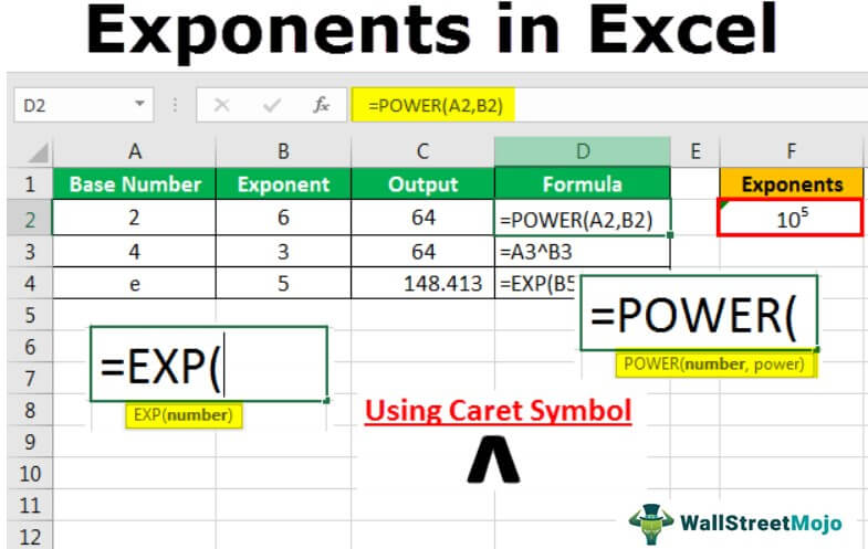
Exponents in Excel are the same exponential function in Excel, such as in Mathematics, where a number is raised to a power or exponent of another number. We can use exponents through the two methods: the POWER function in the Excel worksheet takes two arguments, one as the number and another as the exponent, or we can use the exponent symbol from the keyboard.
Table of contents
You are free to use this image on your website, templates, etc., Please provide us with an attribution link How to Provide Attribution? Article Link to be Hyperlinked
For eg:
Source: Exponents in Excel (wallstreetmojo.com)
How to Use Exponents in Excel Formula?
The following are the methods we can use exponents in the Excel formula.
Method #1 – Using the Power Function
The POWER formula should start with the “=” sign.
The formula of the POWER function is:
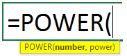
- Number: It is the base number.
- Power: It is the exponent.
Below are simple examples of using the POWER function.

The result is shown below.

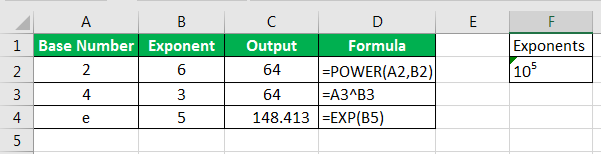
The first row has the base number of 6 and exponent as 3, which is 6 x6 x 6, and the result is 216, which can be derived using a POWER function in Excel.
We can use the formula’s base number and the exponents directly instead of the cell reference(as shown in the example below).
5 is multiplied twice in the first row, 5 x 5.
The result is 25.
We can use the POWER function to find out the number’s square root, cube root, or nth root. The exponents used to find the square root is (1/2), the cube root is (1/3), and the nth root is (1/n). The nth number means any given number. Below are a few examples.
In this table, the first row has the base number of 49, which is the square root of 7 (7 x 7) and 125 is the cube root of 5 (5 x5 x5), and 244 is the 6th root of 2.5 (2.5 x 2.5 x 2.5 x 2.5 x 2.5 x 2.5).
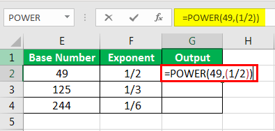
The results are given below.
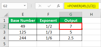
The output column shows the results.

The first row in the above table finds the square root. Then, the second row is for the cube root. Finally, the third row is the nth root of the number.
Method #2 – Using Base Power
The POWER function can be applied using the “caret” symbol, the base number, and the exponent. It is a shorthand used for the POWER function.
We can find this caret symbol on the keyboard in the number 6 key (^). We must hold the “Shift” key and “6” to use this symbol. Then, apply the formula: “=Base ^ Exponent.”
As explained above in the previous examples of a POWER function, the caret formula can be applied to take the cell references or by inserting the base number and the exponent with a caret.
The below table shows the example of using cell references with (^).

The result is shown below:

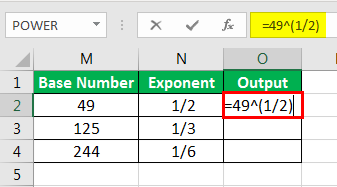
Using the base number and exponent using (^) is shown in the below table.

The result is shown below:

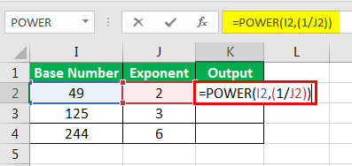
We can use the caret operator to find out the square root, cube root, and nth root of the number where the exponents are (1/2), (1/3), and (1/n) [as shown in the below tables].
Table 1:

Now, the result is shown below:
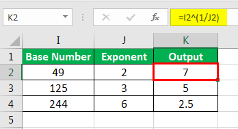
Table 2:
Now, the result is shown below:

Method #3 – Using the EXP Function
Another way of calculating the exponent is by using the EXP function, one of the functions of Excel.
The syntax of the formula is.
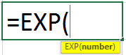
The number is “e,” the base number, and the exponent is the given number. So, it is “e” to the power of a given number. Here, “e” is the constant value, which is 2.718. So, the value of “e” will be multiplied by the times of the exponent (given number).

We can see that the number given in the formula is 5, which means the value of “e,” 2.718, is multiplied 5 times, and the result is 148.413.
Method #4 – Using theText-Based Exponents
We need to use text-based exponents to write or express the exponents. To do this,
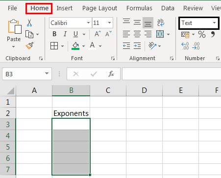
- We must first select the cells where we want to input the exponent’s value. Then, Change the format of the selected cells to Text.
We can do it either by selecting the cells and choosing the Text option from the dropdown list in the Home tab under the Number section or right-clicking on the selected cells and selecting the Format Cells option to select the Text option under Number tab.
Now, we must enter both the base number and exponent in the cell next to next without any space.
We must select the exponent number only (as shown below).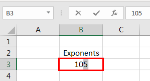
Then, right-click on the cell and select the Format Cells option.
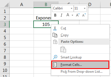
In the pop-up window, check the box for Superscript in excel under the Effects category. Then, press the OK button.
(In Excel, we have an option called Superscript or Subscript to show the mathematical values or formulas).

Click the Enter key. We can see the result below.
All these are examples of how exponents can be expressed in Excel. We can also use this text-based mode of showing the exponents for other mathematical formulas or values.
Below are the ways we can use the exponents in the Excel formula.
Things to Remember
- Whenever the number is shown as the base to the power of the exponent, it may show as text only. We cannot consider this for any numerical calculations.
- When the exponent given in a formula is a large number, the result will be in scientific or exponential notationScientific Or Exponential NotationIn Excel, scientific notation is a specific style of writing numbers in scientific and exponential forms. Scientific notation compactly helps display values, allowing us to compare and use the same in calculations.read more . (e.g., =10^100 provides the result as 1E+100).
- The “Superscript” (to the power of) is an option available in Excel to express the exponents and other mathematical formulas.
- In Excel functions, adding the spaces between the values cannot make any difference. So, we can add a space between the digits for easy readability.
Recommended Articles
This article has been a guide to Exponents in Excel. Here, we discuss using the exponents in Excel formula using caret, EXP, and POWER functions, practical examples, and a downloadable Excel template. You may learn more about Excel from the following articles: –
Источник
Enter a caret — “^” — into the formula bar, then enter the power. For example, to multiply 3 to the power of 4, enter “3^4” and press “Enter” to complete the formula.
Contents
- 1 How does the power function work in Excel?
- 2 How do you write 10 to the power in Excel?
- 3 How do I write mm2 in Excel?
- 4 How do you calculate power in Excel?
- 5 How do you write 10 to the power of 2 in Excel?
- 6 What is E+ Excel?
- 7 What is E 05 Excel?
- 8 How do you write co2 in Excel?
- 9 How do I write a chemical formula in Excel?
- 10 How does excel calculate variance?
- 11 Is m3 cubic meter?
- 12 How do you write 3 cubed?
- 13 How do you write 10 to the power of?
- 14 What does 1e 06 mean in Excel?
- 15 What is E 11 Excel?
- 16 What does 3E mean in Excel?
- 17 What is E 07 Excel?
- 18 What does it mean E 10?
- 19 What is the meaning of E 04?
- 20 How do you write st nd r in Excel?
How does the power function work in Excel?
A Power in Excel is a Math/Trigonometric function computes and returns the result of a number raised to a power. Power Excel function takes two arguments the base (any real number) and the exponent (power, that signifies how many times the given number will be multiplied by itself).
How do you write 10 to the power in Excel?
The power of exponent in Excel is a carot symbol (SHIFT + 6 keyboard shortcut) which is ^. So you will write 10 to the 3rd power in Excel by 10^3. To type exponents in Excel just use carot. In cell you can just write =10^3.
How do I write mm2 in Excel?
To type the 2 Squared Symbol anywhere on your PC or Laptop keyboard (like in Microsoft Word or Excel), press Option + 00B2 shortcut for Mac. And if you are using Windows, simply press down the Alt key and type 0178 using the numeric keypad on the right side of your keyboard.
How do you calculate power in Excel?
Excel POWER Function
- Summary. The Excel POWER function returns a number raised to a given power. The POWER function is an alternative to the exponent operator (^).
- Raise a number to a power.
- Number raised to power.
- =POWER (number, power)
- number – Number to raise to a power. power – Power to raise number to (the exponent).
How do you write 10 to the power of 2 in Excel?
Use the “Power” function to specify an exponent using the format “Power(number,power).” When used by itself, you need to add an “=” sign at the beginning. As an example, “=Power(10,2)” raises 10 to the second power.
What is E+ Excel?
Excel for Microsoft 365 Excel 2021 Excel 2019 Excel 2016 Excel 2013 Excel 2010 Excel 2007 More… The Scientific format displays a number in exponential notation, replacing part of the number with E+n, in which E (exponent) multiplies the preceding number by 10 to the nth power.
What is E 05 Excel?
2.3e-5, means 2.3 times ten to the minus five power, or 0.000023. 4.5e6 means 4.5 times ten to the sixth power, or 4500000 which is the same as 4,500,000.
How do you write co2 in Excel?
Select one or more characters you want to format. Press Ctrl + 1 to open the Format Cells dialog box. Then press either Alt + E to select the Superscript option or Alt + B to select Subscript. Hit the Enter key to apply the formatting and close the dialog.
How do I write a chemical formula in Excel?
When you want to present a formula or an equation for numeric values:
- Click Insert > Equation > Design.
- Click Script and select the format you want.
How does excel calculate variance?
Sample variance formula in Excel
- Find the mean by using the AVERAGE function: =AVERAGE(B2:B7)
- Subtract the average from each number in the sample:
- Square each difference and put the results to column D, beginning in D2:
- Add up the squared differences and divide the result by the number of items in the sample minus 1:
Is m3 cubic meter?
A cubic metre (often abbreviated m3 or metre3) is the metric system’s measurement of volume, whether of solid, liquid or gas. It is also equivalent to 35.3 cubic feet or 1.3 cubic yards in the Imperial system.A cubic metre of water has a mass of 1000 kg, or one tonne.
How do you write 3 cubed?
An easy way to write 3 cubed is 33. This means three multiplied by itself three times. The easiest way to do this calculation is to do the first multiplication (3×3) and then to multiply your answer by the same number you started with; 3 x 3 x 3 = 9 x 3 = 27.
How do you write 10 to the power of?
Thus, shown in long form, a power of 10 is the number 1 followed by n zeros, where n is the exponent and is greater than 0; for example, 106 is written 1,000,000. When n is less than 0, the power of 10 is the number 1 n places after the decimal point; for example, 10−2 is written 0.01.
What does 1e 06 mean in Excel?
1e + 06 means 1 plus 6 zeros. If you wanted to express 2325000 it would have 23.25e+03.
What is E 11 Excel?
It is a notation in Excel. E stands for exponent. 156970000000 is equal to 1.5697E+11 in “E notation” The same number is equal to 1.5697 x 10^11 in “Scientific notation”. You can change the notation by changing number format of the cell.
What does 3E mean in Excel?
Uppercase “E” is the Scientific notation for “10 to the power of”. So -3E-04x is “x times -3 times 10 to the power of -4“, or -0.0003x. Likewise 5E+16e is “5 times 10 to the power of 16, that times e to the power.
What is E 07 Excel?
2 Answers. 1.84E-07 is the exact value, represented using scientific notation, also known as exponential notation. 1.845E-07 is the same as 0.0000001845. Excel will display a number very close to 0 as 0, unless you modify the formatting of the cell to display more decimals.
What does it mean E 10?
E10 means move the decimal to the right 10 places. If the number 1-9 is a whole number, then the decimal may not be seen, but for the purposes of moving the decimal, there is an invisible decimal after each whole number.
What is the meaning of E 04?
The “e” is a symbol for base-10 scientific notation. The “e” stands for ×10exponent. So -1.861246e-04 means −1.861246×10⁻⁴. In fixed-point notation that would be -0.0001861246. This notation is pretty standard.
How do you write st nd r in Excel?
Format dates to include st, nd, rd and th
- 1 Create Custom Number Formats. Highlight the cells to be formatted (B5 to C5) Right-click. Select Format cells. On the Number tab, go to the “Custom” section.
- 2 Conditional Formatting. Click on cell B5. On the Home ribbon, go to Conditional Formatting. Create a New Rule.
In this Excel lesson, you will learn how to use exponents.
Definition
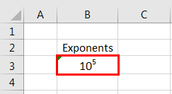
Exponent means how many times the number will be multiplied by itself. For example, 103 (10 to the 3rd power) equals 10 * 10 * 10, which is 1,000.
The power of exponent in Excel is a caret symbol (SHIFT + 6 keyboard shortcut), which is ^. So you will write 10 to the 3rd power in Excel by 10^3.
Calculations
To type exponents in Excel, just use caret.
In the cell, you can just write =10^3.

Of course, a cell address, such as =10^A2, is an option.

Also, =A1^3 is possible.

And =A1^A2 as well.

Excel offers the POWER function for exponent calculations. Write =POWER(10,3) to calculate our example.

You can use the caret or POWER function. Choose the one that you prefer. Maths is much easier with Excel. The ^ operator and the POWER function both perform the same calculation, but the POWER function provides more versatility and control over the calculation, as it allows you to enter the arguments directly into the formula, rather than using the ^ operator.
Further reading:
How to calculate exponential integral
In mathematics, we had exponents, the power to a given base number. In Excel, we have a similar built-in function known as the POWER function, which is used to calculate the power of a given number or base. To use this function, we can use the keyword =POWER( in a cell and provide two arguments, one as the number and another as power.
For example, suppose the base number 4 is raised to the power number 3. i.e., 4 cube. =4*4*4 = 64.
A POWER in Excel is a Math/Trigonometric function that computes and returns the result of a number raised to a power. The POWER Excel function takes two arguments: the base (any real number) and the exponent (power that signifies how many times the given number will be multiplied by itself). For example, 5 multiplied by a power of 2 is the same as 5 x5.
Table of contents
- Power in Excel
- Formula of POWER Function
- Explanation of POWER Function in Excel
- How to Use POWER Function in Excel
- POWER in Excel Example #1
- POWER in Excel Example #2
- POWER in Excel Example #3
- POWER in Excel Example #4
- Recommended Articles
The Formula of POWER Function


Explanation of POWER Function in Excel
The POWER function in Excel takes both arguments as a numeric value. Hence, the arguments passed are of integer type where the number is the base number, and the POWER is the exponent. Both arguments are required and are not optional.


We can use the POWER function in Excel in many ways, like for mathematical operations. For example, we can use the POWER function equation to compute the relational algebraic functions.
How to Use POWER Function in Excel
The Excel POWER function is very simple and easy to use. Let us understand the working of POWER in Excel by some examples.
You can download this POWER Function Excel Template here – POWER Function Excel Template
POWER in Excel Example #1
We have a POWER function equation y=x^n (x to the power n), where y is dependent on the value of x, and n is the exponent. We also want to draw the graph of this f(x, y) function for given values of x and n=2. For example, the values of x are:

So, in this case, since the value of y depends upon the nth power of x, we will calculate the value of Y using the POWER function in Excel.
- 1st value of y will be 2^2 (=POWER(2,2)
- 2nd value of y will be 4^2 (=POWER(4,2)
- ……………………………………………………………
- ……………………………………………………………
- 10th value of y will be 10^2 (=POWER(10,2)

Now, selecting the values of x and y from range B4:K5, choose the graph (in this example, we have chosen the scatter graph with smooth lines) from the “Insert” tab.

So, we get a linear, exponential graph for the given POWER function equation.

POWER in Excel Example #2
In algebra, we have the quadratic POWER function equation, represented as ax2+bx+c=0, where x is unknown, and a, b and c are the coefficients. The solution of this POWER function equation gives the roots of the equation, which are the values of x.
The roots of the quadratic POWER function equation are computed by following mathematical formula:
- x = (-b+ (b2-4ac)1/2)/2a
- x = (-b- (b2-4ac)1/2)/2a
b2-4ac is called discriminant and describes a quadratic POWER function equation’s number of roots.
Now, we have a list of quadratic POWER function equations given in column A. But, first, we need to find the roots of the equations.

^ is the exponential operator used to represent the power (exponent). For example, X2 is the same as x^2.
We have five quadratic POWER function equations, and we will solve them using the formula with the help of the POWER function in Excel to find the roots.
In the first POWER function equation, a=4, b=56, and c = -96. If we mathematically solve them using the above formula, we have the roots -15.5 and 1.5.

To implement this in Excel formula, we will use the POWER function in Excel and the formula will be:
- =((-56+POWER(POWER(56,2)-(4*4*(-93)),1/2)))/(2*4) will give the first root and
- =((-56-POWER(POWER(56,2)-(4*4*(-93)),1/2)))/(2*4) will give the second root of the equation
So, the complete formula will be,
=”Roots of equations are”&” “&((-56+POWER(POWER(56,2)-(4*4*(-93)),1/2)))/(2*4)&” , “&((-56-POWER(POWER(56,2)-(4*4*(-93)),1/2)))/(2*4)
The formulas are concatenated with the string “Roots of equation are.”
Using the same formula for other POWER function equations, we have:

Output:

POWER in Excel Example #3
So, we can use the POWER function in Excel for different mathematical calculations.
Suppose we have to find out the compound interestCompound interest is the interest charged on the sum of the principal amount and the total interest amassed on it so far. It plays a crucial role in generating higher rewards from an investment.read more for which the formula is:
Amount = Principal (1 + r/n)nt
- Where r is the interest rate, n is the number of times interest is compounded per year, and t is the time.
- If an amount of $4,000 is deposited into an account (saving) at an interest rate of 5% annually, compounded monthly, the value of the investment after 5 years can be calculated using the above compound interest formula.
- When, Principal = $4000, rate = 5/100 that is 0.05, n =12 (compounded monthly), time =5 years.
We have the formula using the compound interest formula and implementing it into the Excel formula using the POWER function.
=B2*(POWER((1+(B3/B5)),(B4*B5)))
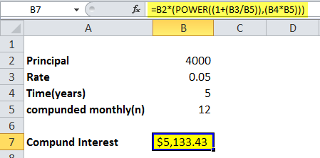
So, the investment balance after 5 years is $5.133.43.
POWER in Excel Example #4
According to Newton’s gravitation law, two bodies at a distance of r from their center of gravity attract each other in the universe according to a gravitational POWER Excel formula.
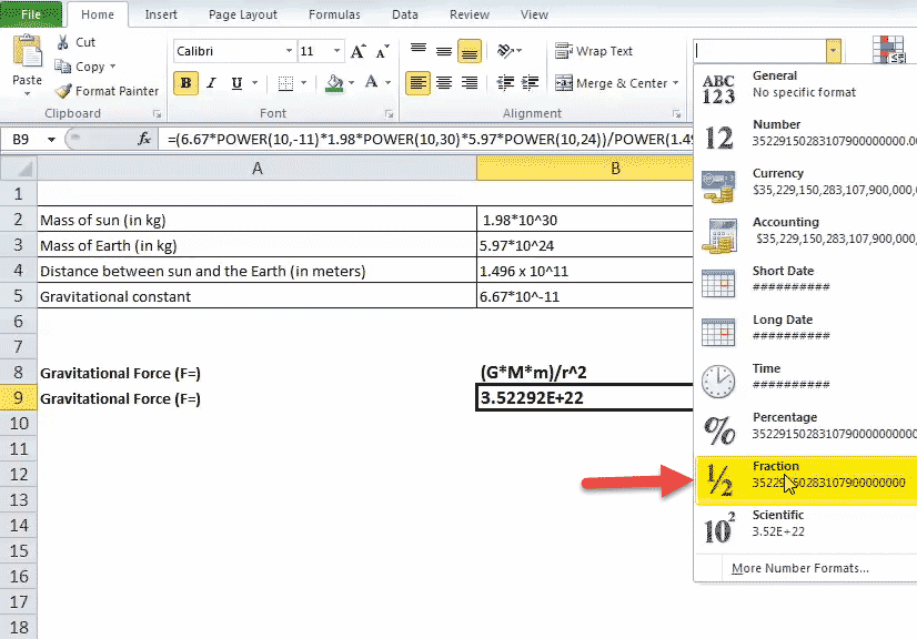
F = (G*M*m)/r2
When F is the magnitude of the gravitational force, G is called the gravitational constant, M is the mass of the first body, m is the mass of the second body, and r is the distance between the bodies from their center of gravity.
Let us calculate the magnitude of gravitational force by which the sun pulls the earth.
- The mass of the sun is 1.98*10^30 kg.
- The mass of the earth is 5.97*10^24 kg.
- The distance between the sun and the earth is 1.496 x 10^11 meters.
- Gravitational constant value is 6.67*10^-11 m3kg-1s-2.
In Excel, if we want to calculate the gravitational force, we will again be using the POWER in Excel that can operate over big numeric values.
- So, we can convert the scientific notation values into the POWER Excel formula using the POWER in Excel.
- 1.98*10^30 will be represented as 1.98*Power(10,30), similarly to other values.
- So, the POWER Excel formula to calculate the force will be: = (6.67*POWER(10,-11)*1.98*POWER(10,30)*5.97*POWER(10,24))/POWER(1.496*POWER(10,11),2)

Since the value obtained as force is a big number Excel expressed it scientific notationIn Excel, scientific notation is a specific style of writing numbers in scientific and exponential forms. Scientific notation compactly helps display values, allowing us to compare and use the same in calculations.read more. To change it into a fraction, change the format to the fraction.
Output:
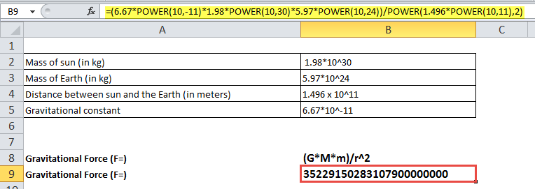
So, the sun pulls the earth with a force of magnitude 35229150283107900000000 Newton.
Recommended Articles
This article is a guide to the POWER Function in Excel. Here, we discuss the POWER formula in Excel and how to use the POWER Excel function, along with Excel examples and downloadable Excel templates. You may also look at these useful functions in Excel: –
- Excel vs. AccessExcel and Access are two of Microsoft’s most powerful tools for data analysis and report generation, but there are some significant differences between them. Excel is an older product of Microsoft, whereas Access is the most advanced and complex product of Microsoft. Excel is very easy to create dashboards and formulas, whereas Access is very easy for databases and connections.read more
- GetPivotData in Excel
- NOT Function