How to take in excel

Windows: 2208 (сборка 15601)
Mac: 16.65 (сборка 220911)
Веб: представлено 15 сентября 2022
г.
iOS: 2.65 (сборка 220905)
Android: 16.0.15629

Возвращает указанное количество непрерывных строк или столбцов с начала или конца массива.

Синтаксис

=TAKE(массив; строки;[столбцы])

Синтаксис функции TAKE поддерживает следующие аргументы.

• массив.    Массив, из которого нужно взять строки или столбцы.

• строки.    Количество строк, которые нужно взять. Отрицательное значение означает взятие с конца массива.

• столбцы.  Количество столбцов, которые нужно взять. Отрицательное значение означает взятие с конца массива.

Ошибки

• Excel возвращает #CALC! ошибка указания пустого массива, когда строки или столбцы равны 0. 

• Excel возвращает ошибку #ЧИСЛО, если массив слишком велик.

Примеры

Скопируйте образец данных из следующей таблицы и вставьте его в ячейку A1 нового листа Excel. При необходимости можно отрегулировать ширину столбцов, чтобы видеть все данные.

Возвращает первые две строки из массива в диапазоне A2:C4.

Данные
1	2	3
4	5	6
7	8	9
Формулы
=TAKE(A2:C4;2)

Возвращает первые два столбца из массива в диапазоне A2:C4.

Данные
1	2	3
4	5	6
7	8	9
Формулы
=TAKE(A2:C4;;2)

Возвращает две последние строки массива в диапазоне A2:C4.

Данные
1	2	3
4	5	6
7	8	9
Формулы
=TAKE(A2:C4;-2)

Возвращает первые две строки и столбца из массива в диапазоне A2:C4.

Данные
1	2	3
4	5	6
7	8	9
Формулы
=TAKE(A2:C4;2;2)

См. также

Функция TOCOL

Функция ВСТРОКУ

Pin

Excel is a spreadsheet program that is developed for Windows, Mac, Android, and iOS. It helps to perform calculations on your PC. The purpose of this software is to do complicated calculations which are difficult to do manually. Sometimes, we want to extract the specified number of rows and columns from the range, for that we can use this TAKE function.

Here we will show you how to use the Excel TAKE function in the worksheet using its basic syntax, explanation, and proper examples. Get an official version of MS Excel from the following link: 

https://www.microsoft.com/en-in/microsoft-365/excel

Pin

Jump To

• Definition of TAKE Function
• Syntax
• Examples
• Wrap-Up
• Video Tutorial

Definition of TAKE Function

• It is one of the built-in functions in Microsoft Excel.
• The TAKE function returns a subset of a given array. By using this function, we can extract the specified number of rows and columns from the range.

Syntax

• Here, you will see the syntax of the TAKE function.
• To apply this function on your spreadsheet, you must select a cell and enter the formula in the following format.
• Once you enter the formula, click on the Enter button to get the result.

=TAKE (array, [rows], [col])

Syntax Explanation:

• array – The source array or range.
• rows – It is an optional one. A number of rows to return as an integer.
• col – [optional] Number of columns to return as an integer.

Examples

Let’s look at some practical examples of the TAKE Function and explore how to use it in Microsoft Excel.

• Initially, you have to open your Excel workbook on your PC and launch the worksheet with data.
• For example, we have entered the student score details in the range B3:C10. From this range, we will extract the last three rows using the TAKE function.

Pin

• Then, you have to enter the formula in the cell as shown below to get the result.

Pin

• After entering the formula, you need to click the Enter button to get the output.

Pin

• Let’s see another example to make it clear for you. From the same input range, we will extract one column. We have entered the formula, as shown below.

Pin

• After entering the formula, you need to click the Enter button to get the output.

Pin

Wrap-Up

We hope that this post helped you to know how to use the Excel TAKE function in the spreadsheet with a few practical examples. Drop your suggestions in the below comment section. To learn more about Excel functions, then visit our webpage Aawexcel.com.

Video Tutorial

The following video will show you how to apply the TAKE function in your Excel worksheet.

Also Read:

Liked our article?

Hi there, I’m Sridhar – an Excel enthusiast with over 10 years of experience working with software. I’m passionate about using Excel to solve complex problems and streamline business processes. Over the years, I have helped businesses of all sizes to improve their operations and save time and money.

Aside from working with Excel, I also enjoy writing and sharing my knowledge with others. You’ll often find me contributing to the AAW Excel blog, where I provide tips, tricks, and tutorials that are easy to understand for readers of all skill levels.

Excel has a set of TEXT Functions that can do wonders. You can do all kinds of text slice and dice operations using these functions.

One of the common tasks for people working with text data is to extract a substring in Excel (i.e., get psrt of the text from a cell).

Unfortunately, there is no substring function in Excel that can do this easily. However, this could still be done using text formulas as well as some other in-built Excel features.

Let’s first have a look at some of the text functions we will be using in this tutorial.

Excel TEXT Functions

Excel has a range of text functions that would make it really easy to extract a substring from the original text in Excel. Here are the Excel Text functions that we will use in this tutorial:

• RIGHT function: Extracts the specified numbers of characters from the right of the text string.
• LEFT function: Extracts the specified numbers of characters from the left of the text string.
• MID function: Extracts the specified numbers of characters from the specified starting position in a text string.
• FIND function: Finds the starting position of the specified text in the text string.
• LEN function: Returns the number of characters in the text string.

Extract a Substring in Excel Using Functions

Suppose you have a dataset as shown below:

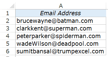
These are some random (but superhero-ish) email ids (except mine), and in the examples below, I’ll show you how to extract the username and domain name using the Text functions in Excel.

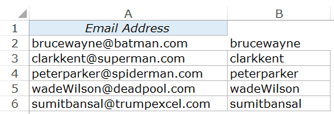
Example 1 – Extracting Usernames from Email Ids

While using Text functions, it is important to identify a pattern (if any). That makes it really easy to construct a formula. In the above case, the pattern is the @ sign between the username and the domain name, and we will use it as a reference to get the usernames.

Here is the formula to get the username:

=LEFT(A2,FIND("@",A2)-1)

The above formula uses the LEFT function to extract the username by identifying the position of the @ sign in the id. This is done using the FIND function, which returns the position of the @.

For example, in the case of brucewayne@batman.com, FIND(“@”,A2) would return 11, which is its position in the text string.

Now we use the LEFT function to extract 10 characters from the left of the string (one less than the value returned by the LEFT function).

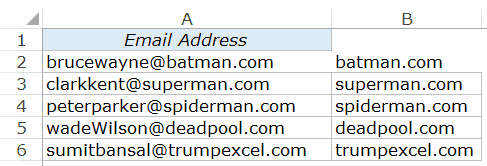
Example 2 – Extracting the Domain Name from Email Ids

The same logic used in the above example can be used to get the domain name. A minor difference here is that we need to extract the characters from the right of the text string.

Here is the formula that will do this:

=RIGHT(A2,LEN(A2)-FIND("@",A2))

In the above formula, we use the same logic, but adjust it to make sure we are getting the correct string.

Let’s again take the example of brucewayne@batman.com. The FIND function returns the position of the @ sign, which is 11 in this case. Now, we need to extract all the characters after the @. So we identify the total length of the string and subtract the number of characters till the @. It gives us the number of characters that cover the domain name on the right.

Now we can simply use the RIGHT function to get the domain name.

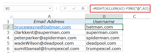
Example 3 – Extracting the Domain Name from Email Ids (without .com)

To extract a substring from the middle of a text string, you need to identify the position of the marker right before and after the substring.

For example, in the example below, to get the domain name without the .com part, the marker would be @ (which is right before the domain name) and . (which is right after it).

Here is the formula that will extract the domain name only:

=MID(A2,FIND("@",A2)+1,FIND(".",A2)-FIND("@",A2)-1) 

Excel MID function extracts the specified number of characters from the specified starting position. In this example above, FIND(“@”,A2)+1 specifies the starting position (which is right after the @), and FIND(“.”,A2)-FIND(“@”,A2)-1 identifies the number of characters between the ‘@‘ and the ‘.‘

Update: One of the readers William19 mentioned that the above formula wouldn’t work in case there is a dot(.) in the email id (for example, bruce.wayne@batman.com). So here is the formula to deal with such cases:

=MID(A1,FIND("@",A1)+1,FIND(".",A1,FIND("@",A1))-FIND("@",A1)-1)

Using Text to Columns to Extract a Substring in Excel

Using functions to extract a substring in Excel has the advantage of being dynamic. If you change the original text, the formula would automatically update the results.

If this is something you may not need, then using the Text to Columns feature could be a quick and easy way to split the text into substrings based on specified markers.

Here is how to do this:

This will instantly give you two sets of substrings for each email id used in this example.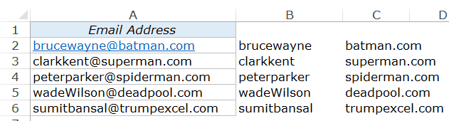

If you want to further split the text (for example, split batman.com to batman and com), repeat the same process with it.

Using FIND and REPLACE to Extract Text from a Cell in Excel

FIND and REPLACE can be a powerful technique when you are working with text in Excel. In the examples below, you’ll learn how to use FIND and REPLACE with wildcard characters to do amazing things in Excel.

See Also: Learn All about Wildcard Characters in Excel.

Let’s take the same Email ids examples.

Example 1 – Extracting Usernames from Email Ids

Here are the steps to extract usernames from Email Ids using the Find and Replace functionality:

This will instantly remove all the text before the @ in the email ids. You’ll have the result as shown below:

How this works?? – In the above example, we have used a combination of @ and *. An asterisk (*) is a wildcard character that represents any number of characters. Hence, @* would mean, a text string that starts with @ and can have any number of characters after it. For example in brucewayne@batman.com, @* would be @batman.com. When we replace @* with blank, it removes all the characters after @ (including @).

Example 2 – Extracting the Domain Name from Email Ids

Using the same logic, you can modify the ‘Find what’ criteria to get the domain name.

Here are the steps:

This will instantly remove all the text before the @ in the email ids. You’ll have the result as shown below:

You May Also Like the Following Excel Tutorials:

• How to Count Cells that Contain Text Strings.
• Extract Usernames from Email Ids in Excel [2 Methods].
• Excel Functions (Examples + Videos).
• Get More Out of Find and Replace in Excel.
• How to Capitalize First Letter of a Text String in Excel
• How to Extract the First Word from a Text String in Excel
• Separate Text and Numbers in Excel

In various activities it is necessary to calculate percentages. We should understand, how do we «get» them. Trade allowances, VAT, discounts, profitability of deposits, securities and even tips — all these are calculated in the form of some part from the whole.

Let’s figure out how to work with the percentages in Excel. This program calculates automatically and admits different variants of the same formula.



Working with percentages in Excel

To count the percentage of the number, add, and take percentages on a modern calculator is not difficult. The main condition is the corresponding icon (%) on the keyboard. And only then it’s the matter of technology and mindfulness.

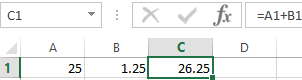
For example 25 + 5%. To find the value of the expression, you need to type on the calculator a given sequence of numbers and signs. The result is 26.25. With such a technique the great intellect is not needed.

To formulate formulas in Excel, let us recollect the school basics:

Percentage is one hundredth part of the whole.

To find a percentage of an integer, we should divide the required fraction by an integer and multiply by 100.

Example: 30 pieces of goods were bought. On the first day 5 units were sold. How many percentages of goods were sold?

5 is a part. 30 is an integer. We substitute data into the formula:

(5/30) * 100 = 16.7%

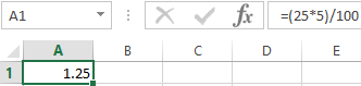
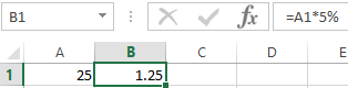
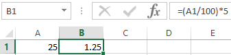
To add a percentage to a number in Excel (25 + 5%), you must first find 5% of 25. At school there was the proportion:

• 25 — 100%;
• Х — 5%.

X = (25 * 5) / 100 = 1.25

After that you can perform the addition. When the basic computing skills are restored, it is easy to understand the formulas.



How to calculate the percentage from the number in Excel

There are several ways.

Adapt the mathematical formula to the program: (Part / Whole) * 100.

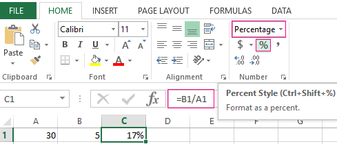
Look attentively at the formula line and the result. The result turned out to be correct. But we did not multiply by 100. Why?

In Excel the format of the cells changes. For C1, we have assigned a «Percentage» format. It means multiplying the value by 100 and putting it on the screen with the sign %. If necessary, you can set a certain number of digits after the decimal point.

Now let’s calculate how much will be 5% of 25. To do this, enter the formula in the cell: = (25 * 5) / 100. The result is:

Another variant is = (25/100) * 5. The result will be the same.

Let’s have the example in another way by using the % sign on the keyboard:

Let us apply this knowledge to practice.

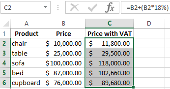
The cost of the goods and the VAT rate (18%) are known. We need to calculate the amount of VAT.

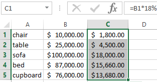
We multiply the cost of goods by 18%. Copy the formula for the whole column. To do this, we catch the mouse with the lower right corner of the cell and pull it down.

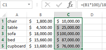
The amount of VAT, the rate is known. We should find the value of the goods. Calculation formula is: = (B1 * 100) / 18. The result is:

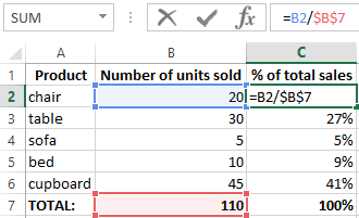
The quantity of the sold goods is known, separately and the whole. It is necessary to find the share of sales for each unit relative to the whole. The calculation formula remains the same: Part / Whole * 100. Only in this example we make the reference to the cell in the denominator of the fraction absolute. Use the $ sign in front of the line name and column name: $B$7.

How to add the percent to number

The task is solved in two actions:

1. Firstly, we find how much a percentage of the number is. Here we calculated how much will be 5% of 25.



2. Secondly, we add the result to the number. Example for review: 25 + 5%.

And here we performed the actual addition. Omit the intermediate effect.

The VAT rate is 18%. We need to find the amount of VAT and add it to the price of the goods. The formula is: =price + (price * 18%).

Do not forget about the brackets! With the help of it we establish the calculation procedure.

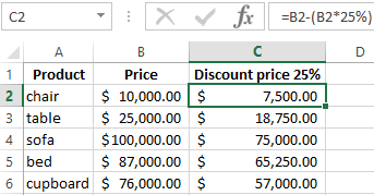
To remove the percentage from a number in Excel, you should follow the same procedure. We perform subtraction instead of addition.

How to count the odds in percentage in Excel?

What is the amount of the value changing between the two values in percentage?

First, let’s abstract from Excel. A month ago, the tables were brought to the store at a price of 100$ per unit. Today, the purchase price is 150$.

Difference in percentage is: = (New price – Old price) / Old price * 100%.

In our example, the purchase price for a unit of goods increased in 50%.

Let’s calculate the percentage difference between the data in two columns:

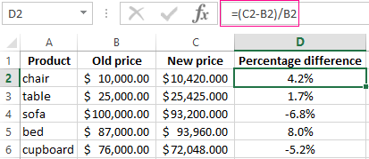
Do not forget to expose the «Percentage» format of the cells. Calculate the percentage difference between the lines:

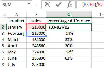
The formula is as follows: =(next value – previous value) / previous value.

With such an arrangement of the data, the first line is skipped!

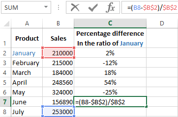
If you want to compare the data for all months with January, for example, use the absolute reference to the cell with the desired value ($ sign).

How to make a diagram with percentages

The first option is to make a column in the data table. Select 2 cell ranges A2:A6 and C2:C6 (while holding down the CTRL key). Then use this data to build a chart. Select the cells with percentages and copy — click «INSERT» — select the type of chart (for example «2D Pie») — OK.

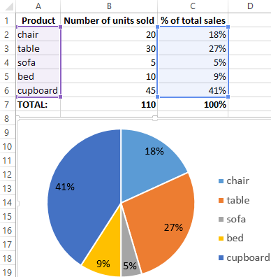
The second option: specify the format of data signatures in the form of a share. There are 22 working shifts in May. You need to calculate the percentage: the amount of work each worker did. We compose the table, where the first column is the number of working days; the second is the number of days off.

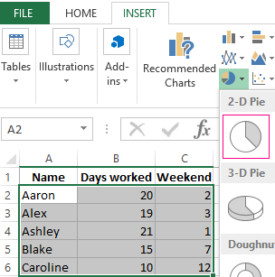
We make a pie chart. Select the data in cell ranges A2:C6. «INSERT» — «Insert Pie or Doughnut Chart» — «2D Pie».

Click on them with the right mouse button — «Add Data Labels» and «Format Data Labels»:

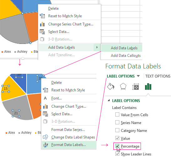
Choose «Share». On the tab «LABEL OPTIONS» we choose the percentage format. It turns out like this:

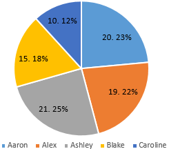
Download examples Calculate Percentages in Excel

We may stop here. And you can edit it to your taste: change the color, the appearance of the diagram, makes underscores and so on.

When using data in Excel that has been imported from another source, the text is often not how you wish to see it.

You may find that product references consist of a product code, code reference, and product size all concatenated into one piece of text which appears in one cell within the worksheet.

Your requirement is that you want to split the relevant sections of the text string so that they all appear in individual cells in your worksheet.

This may be because you want to sort or group by a particular section of text. You may also want to use other formulae on that particular split section. For example, you may want to do a lookup on another table of data, using that section of text as the lookup value. This would be impossible with the data in its original form.

If you are using the data in a pivot table, you may require a separate field that has the split data in order to allow filtering or consolidation.

This article describes seven ways in which you can extract the first or last N characters from a string of text data in Microsoft Excel.

Sample Data Used in this Post

The examples in this post will extract the first and last 2 characters from the ProductSKU in the above set of small product data. The first 2 characters in the SKU contains the product category code and the last 2 characters contains the product size.

Extract Characters with LEFT and RIGHT functions

Excel has several useful functions for splitting strings of text to get at the actual text that you need.

LEFT Function

Syntax:

LEFT ( Text, [Number] )

• Text – This is the text string that you wish to extract from. It can also be a valid cell reference within a workbook.
• Number [Optional] – This is the number of characters that you wish to extract from the text string. The value must be greater than or equal to zero. If the value is greater than the length of the text string, then all characters will be returned. If the value is omitted, then the value is assumed to be one.

This will return the specified number of characters from the text string, starting at the left-hand side of the text. It will extract the first specified number of characters from the text.

RIGHT Function

Syntax:

RIGHT ( Text, [Number] )

The parameters work in the same way as for the LEFT function described above.

This will return the specified number of characters from the text string, starting at the right-hand side of the text. It will extract the last specified number of characters from the text.

Extract Characters with Text to Column

Text to Columns allows you to split a column into sections by defining fixed limits to your text section. To use this methodology:

1. Select all the data in the ProductSKU column in the sample data.
2. Click on the Data tab in the Excel ribbon.
3. Click on the Text to Columns icon in the Data Tools group of the Excel ribbon and a wizard will appear to help you set up how the text will be split.
4. Click on the Fixed Width option button.
5. Click on Next for the next step of the wizard.

In the second step, in the Preview Window, click on the measuring bar in Data Preview where you want to divide the text. This will display a vertical line showing the separation. Do this again for the right-hand characters.

Click on Next to go to the final step of the wizard.

Set the destination cell to E3, so that existing data does not get overwritten.

Click Finish and your data will be imported into three columns commencing at cell E3.

Your worksheet will now look like above with the results split into separate cells.

Extract Characters with Flash Fill

This Flash Fill methodology allows you to enter a couple of examples into the cells where you want your split data to appear. Excel then works out what data is needed in the column based on your examples.

The disadvantage of this methodology is that the examples dictate how many characters will be extracted. This works well if it is always a uniform number, but in some cases, it may not be, in which case this will not work.

To use Flash Fill, you need to enter at least three examples of the text that you wish to see.

You can also activate Flash Fill in the Data Tools group of the Data tab on the Excel ribbon or by using the Ctrl + E keyboard shortcut.

Excel will then automatically fill in the remaining data based on your examples.

Extract Characters with VBA

VBA is the programming language that sits behind Excel and allows you to write your own code to manipulate data, or to even create your own functions.

To access the Visual Basic Editor (VBE), you use ALT + F11.

Sub SplitText()
Dim N As Integer
For N = 3 To 12
    ActiveSheet.Cells(N, 5).Value = Left(Cells(N, 2), 2)
Next N
End Sub

Inside the visual basic editor.

1. Click on Insert in the menu bar.
2. Click on Module and a new pane will appear for the module.
3. Paste in the above code.

Your window will now look like above.

Put the cursor anywhere within the code procedure and then press F5 to run the code.

The code loops through the values of 3 to 12, which are the row numbers for the sample data. It enters the first two characters of the text found at the row number N and column 2 into column 5 (column E).

This is very simple VBA code, and it has the disadvantage that it only takes the first two characters of the product code. If the product code is longer then the wrong result will be produced.
However, the code could be extended to search for the delimiter character (-) and then take the number of characters up to that point.

Extract Characters with Power Query

Power Query is a useful tool in Excel for manipulating data, and it can easily be used to split a column of data into sections.

First, you need to convert your data into an Excel table.

Create a From Table/Range query.

1. Select a cell inside the table.
2. Go to the Data tab
3. Click on From Table/Range in the Get & Transform Data group.

This will open up the power query editor which will allow you to transform the data.

1. Click on the ProductSKU column.
2. Click on the Add Column tab of the power query editor.
3. Click on Extract in the From Text group.
4. Select First Characters in the drop-down.

A pop-up window will be displayed. Enter 2 into the Count box. Click on OK and a new column called First Characters will be added. Double-click on the new column header and rename it to Category.

= Table.AddColumn(#"Changed Type", "First Characters", each Text.Start([ProductSKU], 2), type text)

This will result in the above M code formula.

If you need the last 2 characters, then click on Last Characters in the Extract drop-down.

= Table.AddColumn(#"Inserted First Characters", "Last Characters", each Text.End([ProductSKU], 2), type text)

It will result in the above M code formula.

Click on Close and Load in the Close group on the Home tab of the ribbon, and a new worksheet will be added to your workbook with a table of the data in the new format.

Extract Characters with a Power Pivot Calculated Column

You can also use a Power Pivot Table to show the first two characters of the Product Code.

To do this you need to convert your data into an Excel table.

To import your data into Power Pivot:

1. Select a cell inside the table.
2. Go to the Power Pivot tab. If you don’t see the Power Pivot tab, you can install it by going to the Data tab and clicking on Manage Data Model.
3. Select Add to Data Model.

This will open the Power Pivot add-in with the table loaded. You can open this any time from the Power Pivot tab by selecting Manage in the Data Model group in the Excel ribbon.

Right-click on the header for the Add Column and click on Rename Column in the pop-up menu. You can also double click on the column to rename it. Then you can rename this to something like Category.

= LEFT(Products[ProductSKU], 2)

Select any cell inside the new Category column and insert the above formula into the formula bar. Regardless of which cell you enter this formula in, it will propagate throughout the entire column.

The Category column now shows the first two characters of the product code.

= RIGHT(Products[ProductSKU], 2)

You can do the same with the above formula for the last 2 characters.

Click on the Pivot Table icon in the ribbon and click on Pivot Table in the pop-up menu in order to turn your source data into a spreadsheet pivot table.

Specify the location of your pivot table in the first pop-up window and click OK. If the Pivot Table Fields pane does not automatically display, right click on the pivot table skeleton and select Show Field List.

Now you can summarise your data by Category or Size.

In the Pivot Table Fields Pane, double click on your data source name e.g. Products and this will show the available fields. Check all the boxes to use all fields in your pivot table.

In the Rows box, drag the Category field to the top of the list so that the pivot table will summarise by different categories.

All the normal pivot table functionality is available in terms of re-naming columns, formatting numbers, etc.

Extract Characters with a Power Pivot Measure

To use a measure to split the field ProductSKU, you use the same data source instructions as for the Calculated Column methodology shown above.

When you click on the Power Pivot tab and click on the Manage icon, you can enter a Measure into the Power Pivot Manager window.

This window is divided into two sections. The top section shows the source data in the table, and the bottom section shows the measures. These are formulae that use the data in the table, and create a calculated field that can be used within the pivot table.

Category List :=
CONCATENATEX (
    VALUES ( Products[Category] ),
    Products[Category],
    ", "
)

Select the first cell in the measures section and enter the above formula in the formula bar.

A measure always needs to return a scalar value. This is why the CONCATENATEX function is used first in order to aggregate the results of the calculated columns created from the LEFT or RIGHT functions. If the CONCATENATEX function is not present, then this will return an error value and cannot be used in the pivot table.

Click on the Pivot Table icon in the ribbon, and follow the instructions to create the pivot table as shown above in the calculated column example.

In the Pivot Table Fields list, there is now a calculated field called Category, shown with fx in front of it. This returns the first two characters of the field ProductSKU.

Because a measure is always a calculated field, it can only be included as a value, even though it actually returns a text value in this case. It cannot be used as a filter or as a row or column name.

This is a huge disadvantage overusing a calculated column in the Power Pivot.

Conclusion

There are many ways to get the first or last few characters from your text in Excel.

You can use formula, text to column, flash fill, VBA, Power Query, or Power Pivot.

Which one do you prefer?