
SUM function
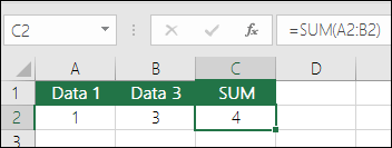
The SUM function adds values. You can add individual values, cell references or ranges or a mix of all three.
For example:
-
=SUM(A2:A10) Adds the values in cells A2:10.
-
=SUM(A2:A10, C2:C10) Adds the values in cells A2:10, as well as cells C2:C10.

SUM(number1,[number2],…)
|
Argument name |
Description |
|---|---|
|
number1 Required |
The first number you want to add. The number can be like 4, a cell reference like B6, or a cell range like B2:B8. |
|
number2-255 Optional |
This is the second number you want to add. You can specify up to 255 numbers in this way. |
This section will discuss some best practices for working with the SUM function. Much of this can be applied to working with other functions as well.
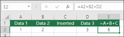
The =1+2 or =A+B Method – While you can enter =1+2+3 or =A1+B1+C2 and get fully accurate results, these methods are error prone for several reasons:
-
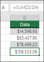
Typos – Imagine trying to enter more and/or much larger values like this:
-
=14598.93+65437.90+78496.23
Then try to validate that your entries are correct. It’s much easier to put these values in individual cells and use a SUM formula. In addition, you can format the values when they’re in cells, making them much more readable then when they’re in a formula.

-
-
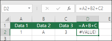
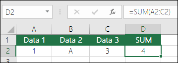
#VALUE! errors from referencing text instead of numbers
If you use a formula like:
-
=A1+B1+C1 or =A1+A2+A3
Your formula can break if there are any non-numeric (text) values in the referenced cells, which will return a #VALUE! error. SUM will ignore text values and give you the sum of just the numeric values.
-
-
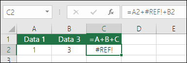
#REF! error from deleting rows or columns
If you delete a row or column, the formula will not update to exclude the deleted row and it will return a #REF! error, where a SUM function will automatically update.
-
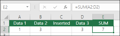
Formulas won’t update references when inserting rows or columns
If you insert a row or column, the formula will not update to include the added row, where a SUM function will automatically update (as long as you’re not outside of the range referenced in the formula). This is especially important if you expect your formula to update and it doesn’t, as it will leave you with incomplete results that you might not catch.
-
SUM with individual Cell References vs. Ranges
Using a formula like:
-
=SUM(A1,A2,A3,B1,B2,B3)
Is equally error prone when inserting or deleting rows within the referenced range for the same reasons. It’s much better to use individual ranges, like:
-
=SUM(A1:A3,B1:B3)
Which will update when adding or deleting rows.
-
-
I just want to Add/Subtract/Multiply/Divide numbers See this video series on Basic Math in Excel, or Use Excel as your calculator.
-
How do I show more/less decimal places? You can change your number format. Select the cell or range in question and use Ctrl+1 to bring up the Format Cells Dialog, then click the Number tab and select the format you want, making sure to indicate the number of decimal places you want.
-
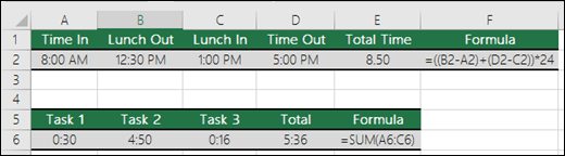
How do I add or subtract Times? You can add and subtract times in a few different ways. For example, to get the difference between 8:00 AM — 12:00 PM for payroll purposes you would use: =(«12:00 PM»-«8:00 AM»)*24, taking the end time minus the start time. Note that Excel calculates times as a fraction of a day, so you need to multiply by 24 to get the total hours. In the first example we’re using =((B2-A2)+(D2-C2))*24 to get the sum of hours from start to finish, less a lunch break (8.50 hours total).
If you’re simply adding hours and minutes and want to display that way, then you can sum and don’t need to multiply by 24, so in the second example we’re using =SUM(A6:C6) since we just need the total number of hours and minutes for assigned tasks (5:36, or 5 hours, 36 minutes).
For more information, see: Add or subtract time.
-
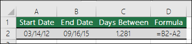
How do I get the difference between dates? As with times, you can add and subtract dates. Here’s a very common example of counting the number of days between two dates. It’s as simple as =B2-A2. The key to working with both Dates and Times is that you start with the End Date/Time and subtract the Start Date/Time.
For more ways to work with dates see: Calculate the difference between two dates.
-
How do I sum just visible cells? Sometimes, when you manually hide rows or use AutoFilter to display only certain data you also only want to sum the visible cells. You can use the SUBTOTAL function. If you’re using a total row in an Excel table, any function you select from the Total drop-down will automatically be entered as a subtotal. See more about how to Total the data in an Excel table.
Need more help?
You can always ask an expert in the Excel Tech Community or get support in the Answers community.

See Also
Learn more about SUM
The SUMIF function adds only the values that meet a single criteria
The SUMIFS function adds only the values that meet multiple criteria
The COUNTIF function counts only the values that meet a single criteria
The COUNTIFS function counts only the values that meet multiple criteria
Overview of formulas in Excel
How to avoid broken formulas
Find and correct errors in formulas
Math & Trig functions
Excel functions (alphabetical)
Excel functions (by Category)
Need more help?
Want more options?
Explore subscription benefits, browse training courses, learn how to secure your device, and more.
Communities help you ask and answer questions, give feedback, and hear from experts with rich knowledge.
![]()
Download Article
Simple and advanced methods to sum in Excel
![]()
Download Article
- Using the Plus Sign (+)
- Using the SUM Function
- Using the SUMIF Function
- Using the SUMIFS Function
- Q&A
- Tips
|
|
|
|
|
Whether you’re working with a few numbers or large datasets, there’s a Microsoft Excel summation formula for you! The most common adding function is “=SUM()”, with the target cell range placed between the parentheses. But, there are various ways to add numbers in your spreadsheet. This wikiHow guide will show you how to use summation formulas in Microsoft Excel. We’ll cover 4 methods: the plus sign operator (+), =SUM, =SUMIF, and =SUMIFS.
Things You Should Know
- For small-scale addition, use “=cell1 + cell2 + cell3 + …” to sum cell values.
- For larger sets of data, use “=SUM(your numbers here)” to sum a range of values
- To add values if they meet one criterion, use “=SUMIF(range, criteria, [sum_range])” where sum_range is optional.
- To add values if they meet multiple criteria, use “=SUMIFS(sum_range, criteria_range1, criteria1, [criteria_range2, criteria2], …)”.
Choose a Method
- Plus sign: Simple and intuitive, but inefficient. Best for small, quick sums.
- SUM function: Useful for large spreadsheets as it can sum a range of cells. Can only accept numeric arguments, not conditional values.
- SUMIF function: Allows you to specify a condition, and only sum values that meet that condition.
- SUMIFS function: Allows for complex logical statements by setting multiple criteria. Not available for Excel 2003 or earlier.
-
1
Enter the formula into a new cell. Make a new spreadsheet. Then, select a cell and type an equals sign (=). Then, alternate between clicking a cell with a value, and typing “+”. Your formula should end with the final cell you want to sum. Your finished formula should look like cell1 + cell2 + cell3. Hit the Enter key when you complete your formula.
- For example, =C4+C5+C6+C7 will sum the values of the four cells, C4, C5, C6, and C7.
- Each time you click on another cell, Excel will insert the cell reference for you (C4, for example), which tells Excel which spreadsheet cell contains the number (for C4, it’s the cell in column C, in row 4).
- If you know which cells you want to calculate, you can type them out instead of clicking them individually.
- Excel functions will recognize a combination of numbers and cell references in formulas. For example, you could type “=5000+C5+25.2+B7”.
- If you’re looking for subtraction information, check out our guide on how to subtract in Excel.

Advertisement
-
1
Use the SUM function to add two or more cells. Select the cell you want the summation to output to. Then, type an equals sign (=), SUM, and the cells you’re summing enclosed in parenthesis. The function should look like this: =SUM(your numbers here).
- For example, =SUM(C4,C5,C6,C7) will add the numbers contained in the 4 cells within the parentheses.
-
2
Use the SUM function to add a range of cells. If you provide a starting and ending cell, separated by a colon (:), you can sum large sections of the spreadsheet. The function should look like this: =SUM(cell1:cell2)’ where “cell1” and “cell2” are your starting and ending cell respectively.
- For example, =SUM(C4:C7) sums the values in C4 to C7.
- You don’t have to type out “C4:C7”. After typing “=SUM(” you can select a range by clicking and dragging your cursor from cell C4 to C7. The range will appear in the formula following the open parenthesis. Add the closing parenthesis at the end, and you’re done!
- For a large range of numbers, this is much faster than clicking on each cell individually.
-
3
Use the AutoSum Wizard. If you’re using Excel 2007 or later, an alternative to typing “=SUM” is using AutoSum.[1]
- Select the cell you want the summation to output to.
- Go to the Format tab > AutoSum drop-down arrow > Sum.
- Select the range of cells you want to sum.
- AutoSum might be limited to contiguous cell ranges in some versions of Excel; if you want to skip cells in your calculation, it may not work correctly.
-
4
Copy/paste data into other cells. Since the cell with the function holds both the sum value and the sum function, you have to consider which you want copied.
- Copy the cell with the summation by pressing Ctrl + c (Windows) or Cmd + c (Mac). Then, select another cell and go to the Home tab > Clipboard drop-down and select either Paste Formulas or Paste Values.
-
5
Reference sums in other functions. You can use the value of your summation cell in other functions. Rather than making a new summation or typing out the number value of your previous function, you can reference the original sum cell in other calculations.
- For example, let’s say you create a summation function for column C in C20 and column D in D20. You can add these sums by selecting a new cell and typing “=SUM(C20, D20)”
- This essentially nests your two summations into a third summation formula. Then, if your summation of C or D changes, this third summation will automatically update.


Advertisement
-
1
Use the basic SUMIF function. The SUMIF function allows you to sum values when they meet a criteria. The criteria can be within the range of values itself, or in a different range that is the same size as the values range. If the criteria is in the range itself, follow these steps:[2]
- Type =SUMIF( in a new cell.
- Select or type the range of cells you want to sum, then type a comma (,).
- Type a numerical criteria in double quotation marks, then type a closing parenthesis.
- For example, if you want to only sum numbers in a range that are greater than 10, you could type “=SUM(C1:C10, “>10”)”
-
2
Set up your data for SUMIF. If you’re using the optional parameter [sum_range], you’ll need separate columns for the range you want compared to the criteria and the range you want to sum. There are multiple ways to format a spreadsheet, but here’s a basic setup for SUMIF:
- Create one column with number values and a second column with a conditional value, like “yes” and “no”.
- For example, a column with 4 rows with values 1, 2, 3, and 4 and a second column with values of “yes” or “no”.
- This setup is similar to using VLOOKUP.
-
3
Enter the function into a cell. To create a SUMIF formula using the optional [sum_range], follow these steps:
- Select a new cell and enter “=SUMIF(”
- range — Select or type a range of values to compare to the criteria. Then type a comma (,). This will be the range in the column where you placed your conditional values.
- criteria — Type in the criteria. This can be numerical, text-based, or boolean (TRUE/FALSE). Enclose this criteria with double-quotation marks. Then type a comma (,).
- sum_range — Select or type a range of values to sum. This will be the column you created with number values.
- The sum_range argument should be the same shape and size as range. The SUMIF formula will check the value in each range cell and add the respective sum_range cell to the sum.
- For example: “=SUMIF(C1:C4, “yes”, B1:B4)” will sum values in the range B1:B4 if the cell in C1:C4 is the string “yes”.


Advertisement
-
1
Setup your data table. The setup is similar to SUMIF, but can support multiple criteria with multiple ranges.[3]
- Create one column with number values. These are the values you’ll sum if the criteria in the criteria ranges are met.
- Create multiple columns containing conditional values (e.g. yes/no, TRUE/FALSE, locations, dates, numeric values).
-
2
Enter your SUMIFS function. To create a SUMIFS formula using multiple criteria, follow these steps:
- Select a new cell and enter “=SUMIFS(”
- sum_range — Select or type a range of cells to sum. Then type a comma (,). This will be the range in the column where you typed your number values.
- criteria_range1 — Select or type a range of values to compare to criteria1. Then type a comma (,). This will be one range in a column where you placed conditional values.
- criteria1 — Type in a criteria. This can be numerical, text-based, or boolean (TRUE/FALSE). Enclose this criteria with double-quotation marks. Then type a comma (,).
- criteria_range2 — Select or type a range of values to compare to criteria2. Then type a comma (,). This will be the second range in a column where you placed conditional values.
- criteria2 — Type in a criteria. This can be numerical, text-based, or boolean (TRUE/FALSE). Enclose this criteria with double-quotation marks. Then type a comma (,).
- Continue creating additional criteria_range and criteria as needed.
- The sum_range argument should be the same shape and size as every criteria_range. The SUMIFS formula will check the value in each criteria_range cell and add the respective sum_range cell to the sum.
- For example: “=SUMIFS(B1:B4, C1:C4, “yes”, D1:D4, “california”)” will sum values in the range B1:B4 if the cell in C1:C4 is the string “yes” and the cell in D1:D4 is the string “california”.


Advertisement
Add New Question
-
Question
Need help adding results of very long formulas. The SUM works only if written in one single very long line.

You can establish ranges for SUM using a colon (:). This means you can skip all of the cells in between instead of adding them together one by one.
-
Question
What does the number one mean in =$J$1* — E4?
The $ both in front of the J and 1 mean that its reference is ‘locked’. That means if you copy and paste the formula, or use the Excel Fill Handle (the little click-and-drag bit on the bottom-right of a cell when you click on it), the parts that immediately follow the $ stay the exact same. For instance, if it were just $J1, instead of $J$1, copying and pasting it a 4 rows down, the cell reference would be $J4; if it were J$1, copying and pasting it to the left one column would make the cell reference I$1.
Ask a Question
200 characters left
Include your email address to get a message when this question is answered.
Submit
Advertisement
-
There’s no reason to use complex functions for simple math; likewise no reason to use a simple functions when a more complex function will make life simpler. Take the easy road.
-
These summation functions also work in other free spreadsheet software, like Google Sheets.
-
Ready for a computer or laptop upgrade? Check out our coupon site for Samsung and HP for money-saving deals on your next purchase.
Thanks for submitting a tip for review!
Advertisement
About This Article
Article SummaryX
1. Use the SUM function for ranges with numeric data.
2. Use the plus sign for small, quick sums.
3. Use the SUMIF function to specify a condition.
4. Use the SUMIFS function for complex logical statements.
Did this summary help you?
Thanks to all authors for creating a page that has been read 333,672 times.
Is this article up to date?
The SUM function in excel adds the numerical values in a range of cells. Being categorized under the Math and Trigonometry function, it is entered by typing “=SUM” followed by the values to be summed. The values supplied to the function can be numbers, cell references or ranges.
For example, cells B1, B2, and B3 contain 20, 44, and 67 respectively. The formula “=SUM(B1:B3)” adds the numbers of the cells B1 to B3. It returns 131.
The SUM formula automatically updates with the insertion or deletion of a value. It also includes the changes made to an existing cell range. Moreover, the function ignores the empty cells and text values.
Table of contents
- SUM Function in Excel
- The Syntax of the SUM Excel Function
- The Procedure to Enter the SUM Function in Excel
- The AutoSum Option in Excel
- How to Use the SUM Function in Excel?
- Example #1
- Example #2
- Example #3
- Example #4
- Example #5
- The Usage of the SUM Excel Function
- The Limitations of the SUM Function in Excel
- The Nesting of the SUM Excel Function
- Frequently Asked Questions
- SUM Function in Excel Video
- Recommended Articles
The Syntax of the SUM Excel Function
The syntax of the function is shown in the following image:

The function accepts the following arguments:
- Number1: This is the first numeric value to be added.
- Number2: This is the second numeric value to be added.
The “number1” argument is required while the subsequent numbers (“number 2”, “number 3”, etc.) are optional.
The Procedure to Enter the SUM Function in Excel
You can download this SUM Function Excel Template here – SUM Function Excel Template
To enter the SUM function manually, type “=SUM” followed by the arguments.
The alternative steps to enter the SUM excel function are listed as follows:
- In the Formulas tab, click the “math & trig” option, as shown in the following image.
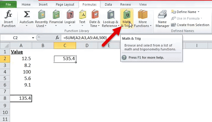
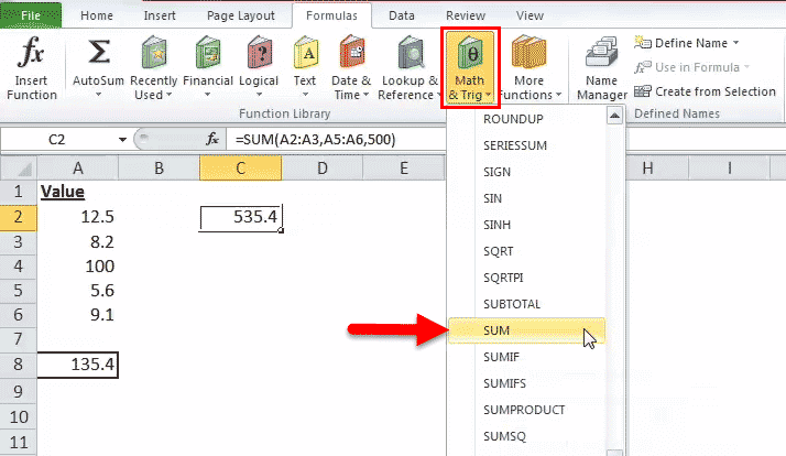
2. From the drop-down menu that opens, select the SUM option.
3. In the “function arguments” dialog box, enter the arguments of the SUM function. Click “Ok” to obtain the output.

The AutoSum Option in Excel
The AutoSum option is the fastest way to add numbers in a range of cells. It automatically enters the SUM formula in the selected cell.
Let us work on an example to understand the working of the AutoSum option. We want to sum the list of values in A2:A7, shown in the succeeding image.
The steps to use the AutoSum command are listed as follows:
- Select the blank cell immediately following the cell to be summed up. Choose the cell A8.

- In the Home tab, click “AutoSum”. Alternatively, press the shortcut keys “Alt+=” together and without the inverted commas.

- The SUM formula appears in the selected cell. It shows the reference of the cells that have been summed up.

- Press the “Enter” key. The output appears in cell A8, as shown in the following image.


How to Use the SUM Function in Excel?
Let us consider a few examples to understand the usage of the SUM function. The examples #1 to #5 show an image containing a list of numeric values.
Example #1
We want to sum the cells A2 and A3 shown in the succeeding image.
Apply the formula “=SUM(A2, A3).” It returns 20.7 in cell C2.

Example #2
We want to sum the cells A3, A5, and the number 45 shown in the succeeding image.
Apply the formula “=SUM (A3, A5, 45).” It returns 58.8 in cell C2.

Example #3
We want to sum the cells A2, A3, A4, A5, and A6 shown in the succeeding image.
Apply the formula “=SUM (A2:A6).” It returns 135.4 in cell C2.

Example #4
We want to sum the cells A2, A3, A5, and A6 shown in the succeeding image.
Apply the formula “=SUM (A2:A3, A5:A6).” It returns 35.4 in cell C2.

Example #5
We want to sum the cells A2, A3, A5, A6, and the number 500 shown in the succeeding image.
Apply the formula “=SUM (A2:A3, A5:A6, 500).” It returns 535.4 in cell C2.

The Usage of the SUM Excel Function
The rules governing the usage of the function are listed as follows:
- The arguments supplied can be numbers, arrays, cell references, constants, ranges, and the results of other functions or formulas.
- While providing a range of cells, only the first range (cell1:cell2) is required.
- The output is numeric and represents the sum of values supplied.
- The arguments supplied can go up to a total of 255.
Note: The SUM excel function returns the “#VALUE!” error if the criterion supplied is a text string longer than 255 characters.
The Limitations of the SUM Function in Excel
The drawbacks of the function are listed as follows:
- The cell range supplied must match the dimensions of the source.
- The cell containing the output must always be formatted as a number.
The Nesting of the SUM Excel Function
The built-in formulas of Excel can be expanded by nesting one or more functions inside another function. This permits multiple calculations to take place in a single cell of the worksheet.
The nested function acts as an argument of the main or the outermost function. Excel calculates the innermost function first and then moves outwards.
For example, the following formula shows the SUM function nested within the ROUND functionThe ROUNDUP excel function calculates the rounded value of the number to the upward side or the higher side. In other words, it rounds the number away from zero. Being an inbuilt function of Excel, it accepts two arguments–the “number” and the “num_of _digits.” For example, “=ROUNDUP(0.40,1)” returns 0.4.
read more:

For the given formula, the output is calculated as follows:
- First, the sum of the values in cells A1 to A6 is computed.
- Next, the resulting number is rounded to three decimal places.
With Microsoft Excel 2007, nested functions up to 64 levels are permitted. Prior to this version, one could nest functions only till 7 levels.
Frequently Asked Questions
1. Define the SUM function of Excel.
The SUM function helps add the numerical values. These values can be supplied to the function as numbers, cell references, or ranges. The SUM function is used when there is a need to find the total of specified cells.
The syntax of the SUM excel function is stated as follows:
“SUM(number1,[number2] ,…)”
The “number1” and “number2” are the first and second numeric values to be added. The “number1” argument is mandatory while the remaining values are optional.
In the SUM function, the range to be summed can be provided, which is easier than typing the cell references one by one. The AutoSum option provided in the Home or Formulas tab of Excel is the simplest way to sum two numbers.
Note: The numeric value provided as an argument can be either positive or negative.
2. How to sum the values of filtered data in Excel?
To add the values of filtered data, use the SUBTOTAL function. The syntax of the function is stated as follows:
“SUBTOTAL(function_num,ref1,[ref2],…)”
The “function_num” is a number ranging from 1 to 11 or 101 to 111. It indicates the function to be used for the SUBTOTALThe SUBTOTAL excel function performs different arithmetic operations like average, product, sum, standard deviation, variance etc., on a defined range.read more. The functions used can be AVERAGE, MAX, MIN, COUNT, STDEV, SUM, and so on.
The “ref1” and “ref2” are the cells or ranges to be added.
The “function_num” and “ref1” arguments are mandatory. The “function_num” 109 is used for adding the visible cells of filtered data.
Let us consider an example.
• The sales revenue generated by A and B of team X are:
$1,240 and $3,562 given in cells C2 and C3 respectively
• The sales revenue generated by C and D of team Y are:
$2,351 and $4,109 given in cells C4 and C5 respectively
We filter only team X rows and apply the formula “SUBTOTAL(109,C2:C3).” It returns $4,802.
Note: Alternatively, the AutoSum property can be used to sum the filtered cells.
3. State the benefits of using the SUM function in Excel.
The benefits of using the SUM function are listed as follows:
• It helps obtain the totals of ranges irrespective of whether the cells are contiguous or non-contiguous.
• It ignores the empty cells and text values entered in a cell. In such cases, it returns an output representing the sum of the remaining numbers of the range.
• It automatically updates to include the addition of a row or a column.
• It automatically updates to exclude the deletion of a row or column.
• It eliminates the difficulty associated with typing manual entries.
• It makes the output more readable by allowing the cell to be formatted as a number.
SUM Function in Excel Video
Recommended Articles
This has been a guide to the SUM function in Excel. Here we discuss how to use Sum Formula along with step by step examples and FAQs. You can download the Excel template from the website. Take a look at these useful functions of Excel–
- SUMIFS with Multiple Criteria
- SUMX in Power BISUMX is a function in power BI which returns the sum of expression from a table. It is an inbuilt mathematical function. The syntax used for this function is SUMX(,).read more
- TEXT Function
- Concatenate Excel Function
- Excel Alternate Row ColorThe two different methods to add colour to alternative rows are adding alternative row colour using Excel table styles or highlighting alternative rows using the Excel conditional formatting option.read more
Reader Interactions
Excel SUM Function (Example + Video)
When to use Excel SUM Function
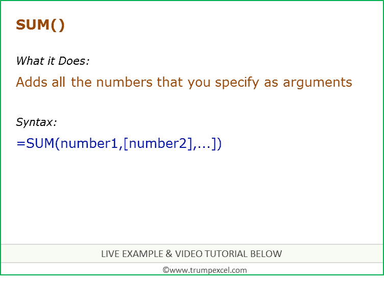
SUM function can be used to add all numbers in a range of cells.
What it Returns
It returns a number that represents the sum of all the numbers.
Syntax
=SUM(number1, [number2],…])
Input Arguments
- number1 – the first number you want to add. It can be a cell reference, a cell range, or can be manually entered.
- [number2] – (Optional) the second number you want to add. It can be a cell reference, a cell range, or can be manually entered.
Additional Notes
- If an argument is an array or reference, only numbers in that array or reference are counted. Empty cells, logical values, or text in the array or reference are ignored
- If any of the argument is an error, it displays an error.
Excel SUM Function – Live Example
Excel SUM Function – Video Tutorial
Related Excel Functions:
- Excel AVERAGE Function.
- Excel AVERAGEIF Function.
- Excel AVERAGEIFS Function.
- Excel SUMIF Function.
- Excel SUMIFS Function.
- Excel SUMPRODUCT Function.
You May Also Like the Following Excel Tutorials:
- Calculate Weighted Average Using Excel Sum Function.
- How to Sum a Column in Excel
- How to Sum time in Excel
- AutoSum in Excel (Shortcut)
SUM Function is a very popular and useful formula in Microsoft Excel. It is one of the most basic, widely used, and easy to understand arithmetic functions in Excel. As the name suggests SUM Function in Excel performs the addition of numbers. Sum Function can accept numbers both as individual arguments and also as a complete range of cells.
How Excel Defines SUM Function
Microsoft Excel defines SUM as a formula that “Adds all the numbers in a range of cells”. This definition clearly points out that the Sum function has a job to add numbers and the arguments can be supplied using combinations of both numbers and the range of cells.
Syntax of SUM Function in Excel
Sum function has two syntaxes and hence they can be written in two different ways:
=SUM( num1, num2, ... num_n )
Here ‘num1’, ‘num2’, and ‘num_n’ specifies numbers which you wish to add.
OR
=SUM(CellRange1,CellRange2, ... CellRange_n)
Here ‘CellRange1’, ‘CellRange2’, ‘CellRange_n’ specifies multiple cell ranges (containing numbers) which are to be added.
Some Important Facts about SUM Formula
- Sum function can also do the addition of decimal numbers and fractions.
- If you are using the SUM formula as =SUM( num1, num2, … num_n ) and in place of ‘num’ you have entered a non-numeric content then the Sum function will throw an #Name? error.
- But if you are using SUM Function as =SUM ( CellRange1, CellRange2, … CellRange_n ) and if any of the cell range contains a non-numeric content then Sum function will ignore this value.
- Sum function is not a dynamic type of function. This means that if you have applied a Sum formula on a range of cells and then you filter out some values then the output of the Sum function won’t change as it doesn’t change its result according to the current values in the filter. It is better to use the Subtotal function in such cases.
Examples of SUM Formula

In the above example, I have applied four types of SUM functions and below I will explain them one by one.
Example 1. In the first example, I have used the SUM function
=SUM(10,11,19)
This Sum function simply adds-up all the values i.e. 10, 11, and 19, and hence the result is 40.
Example 2. In the second example, I have used a function
=SUM(10.2,9.6,2,4)
Simple mathematics can tell us that 10.2+9.6+2.4 is 25.8 and hence the output is 25.8.
Example 3. In the third example, a fraction type Sum function is used as
=SUM(4/2,8/2)
As 4/2 results into 2 and 8/2 results into 4 and the addition of both these give the result 6.
Example 4. In the fourth example, the Sum function is used with a non-numeric value
=SUM(10,EXCEL)
And this is the reason why it results in a #Name? error.

Example 5. In the above image, I have used the second type of SUM function as
=SUM(B2:B10)
to which I have supplied a range of cells (B2:B10) as arguments. This sum function simply adds each element of the range and delivers the result as 60.
Shortcut for Applying SUM Formula in Excel
Instead of applying the sum formula in the normal way, you can also apply the SUM Formula using a shortcut.

Simply select the range (containing your numbers to be added), then press “Alt +” key and the desired sum will be populated in the next cell.
Using Mathematical Operators inside SUM Function
Mathematical operators like (+,-, / and *) can also be used inside Sum functions. This means that a SUM function as:
=SUM(2*4)
is valid and it will result in 8. Similarly, a SUM Function as follows
=SUM(62-4)
is also valid and it results in 58.
Actually, this happens because the Sum Function treats this whole set of numbers and operators as a single expression. So, first of all, it evaluates the result of this mathematical operation, and as there is no other argument supplied to the function so it shows the result as it is.